| Issue |
A&A
Volume 566, June 2014
|
|
|---|---|---|
| Article Number | A59 | |
| Number of page(s) | 22 | |
| Section | Extragalactic astronomy | |
| DOI | https://doi.org/10.1051/0004-6361/201423366 | |
| Published online | 12 June 2014 | |
A simultaneous 3.5 and 1.3 mm polarimetric survey of active galactic nuclei in the northern sky⋆
1 Instituto de Astrofísica de Andalucía (CSIC), Apartado 3004, 18080 Granada, Spain
2 Institute for Astrophysical Research, Boston University, 725 Commonwealth Avenue, Boston, MA 02215, USA
3 Current Address: Joint Institute for VLBI in Europe, Postbus 2, 7990 AA Dwingeloo, The Netherlands
e-mail: This email address is being protected from spambots. You need JavaScript enabled to view it.
4 Instituto de Radio Astronomía Millimétrica, Avenida Divina Pastora, 7, Local 20, 18012 Granada, Spain
5 Max-Planck-Institut für Radioastronomie, Auf dem Hügel, 69, 53121 Bonn, Germany
Received: 2 January 2014
Accepted: 11 April 2014
Abstract
Context. Short millimeter observations of radio-loud active galactic nuclei (AGN) offer an excellent opportunity to study the physics of their synchrotron-emitting relativistic jets from where the bulk of radio and millimeter emission is radiated. On one hand, AGN jets and their emission cores are significantly less affected by Faraday rotation and depolarization than at longer wavelengths. On the other hand, the millimeter emission of AGN is dominated by the compact innermost regions in the jets, where the jet cannot be seen at longer wavelengths due to synchrotron opacity.
Aims. We present the first simultaneous dual frequency 86 GHz and 229 GHz polarimetric survey of all four Stokes parameters for a large sample of 211 radio-loud active galactic nuclei, designed to be flux limited at 1 Jy at 86 GHz.
Methods. Most of the observations were made in mid-August 2010 using the XPOL polarimeter on the IRAM 30 m millimetric radio telescope.
Results. Linear polarization detections above a 3σ median level of ~ 1.0% are reported for 183 sources at 86 GHz and for 23 sources at 229 GHz, where the median 3σ level is ~ 6.0%. We show a clear excess of the linear polarization degree that is detected at 229 GHz with regard to that at 86 GHz by a factor of ~ 1.6. This implies a progressively better ordered magnetic field for blazar jet regions that are located progressively upstream in the jet. We show that the linear polarization angle at 86 and 229 GHz and the jet structural position angle for both quasars and BL Lacs do not show a clear preference to align in either parallel or perpendicular directions. Our variability study with regard to the 86 GHz data from our previous survey points out a large degree of variation. In particular, we report total flux and linear polarization changes in time scales of years by median factors of ~ 1.5 in total flux and ~ 1.7 in linear polarization degree (with maximum variations by factors up to 6.3 and ~ 5, respectively). Moreover, 86% of sources show linear polarization angles evenly distributed with regard to our previous measurements.
Key words: galaxies: active / galaxies: jets / quasars: general / BL Lacertae objects: general / polarization / surveys
Tables 1 and 2 are available in electronic form at http://www.aanda.org
© ESO, 2014
1. Introduction
Among all classes of active galactic nuclei (AGN), radio-loud AGN are characterized by having pairs of relativistic jets of highly energized, magnetized plasma that are ejected along the rotational poles of the super-massive black hole/disk system (e.g., Blandford & Payne 1982). In particular, blazars, the most exotic class of radio-loud AGN, stand out because of the wild variability of their non-thermal jet-emission from radio to γ-rays. Members of this class include BL Lacs and flat spectrum radio quasars (FSRQ, the high power version of the former). The remarkable properties of blazars are affected by strong relativistic effects that beam their radiation and shorten their variability time scales. These properties include superluminal motions (e.g., Gómez et al. 2001; Jorstad et al. 2005; Agudo et al. 2012b), Doppler-boosted emission of the jet pointing at a small angle to the observer (e.g., Kadler et al. 2004), substantial changes in flux and linear polarization, which is sometimes correlated on several spectral ranges on time scales from months (e.g., Bach et al. 2006; Agudo et al. 2011a,b) to hours (e.g., Ackermann et al. 2010; Tavecchio et al. 2010), changes in jet structure (e.g., Jorstad et al. 2007; Agudo et al. 2007), and polarized synchrotron and inverse-Compton emission all along the spectrum (e.g., Marscher et al. 2010; Jorstad et al. 2010; Agudo et al. 2011a,b; Wehrle et al. 2012). The AGN with powerful jets oriented at larger angles to the line of sight (i.e., radio galaxies, the remaining prominent class of radio-loud AGN) suffer less from such relativistic effects; therefore, they display smaller apparent luminosities and longer time scales of variability, although they are thought to be the same astrophysical objects as BL Lacs and FSRQ with the latter being the better oriented counterparts of the former (Urry & Padovani 1995).
Explaining the existence and physical properties of jets from AGN remains one of the greatest current challenges in jet physics. Observations of radio-loud AGN at short millimeter wavelengths offer an excellent opportunity with regard to radio centimeter observations to study these objects for several reasons. First, like AGN radio emission, millimeter emission is well known to be radiated predominantly from the jet with essentially no contribution from the host AGN or its surroundings, which facilitates the interpretation of the measurements in terms of jet physics. Second, AGN jets and, in particular, their millimeter emitting cores are significantly less affected by Faraday rotation and depolarization than at longer wavelengths (see, e.g., Zavala & Taylor 2004; Agudo et al. 2010). Third, the millimeter emission of AGN is dominated by the compact innermost regions in the jets (e.g., Jorstad et al. 2007; Lee et al. 2008), where the jet cannot be seen at longer wavelengths due to synchrotron opacity.
In 2005, we used the XPOL polarimeter (Thum et al. 2008) on the IRAM 30 m telescope to perform the first 3.5 mm (86 GHz) polarization survey of radio-loud AGN over a large (145 source) sample (Agudo et al. 2010). Within the available data, we detected linear polarization above 3σ levels of ~ 1.5% for 76% of the sample. Our results pointed out an excess by a factor of ~ 2 of 86 GHz linear polarization degree with regard to that at radio wavelengths (15 GHz), suggesting that either the region of bulk millimeter emission has a better ordered magnetic field, or that the radio emission is strongly Faraday depolarized with regard to that at millimeter wavelengths. We also reported a trend of decreasing luminosity toward larger linear polarization degrees within our entire sample, which perhaps indicates a lower magnetic field order for larger luminosity jets. Moreover, in contrast to what was found at radio wavelengths (see Lister & Homan 2005, and references therein), we do not find a relation between the linear polarization angle and the jet structural position angle in either quasars or BL Lacs. Confirmation of this result would imply that no AGN class matches the conditions to show linear polarization angles either parallel or perpendicular to the jet. This should mean that they are intrinsically non-axisymmetric.
Aiming to improve the statistical confidence with regard to previous studies, we performed a new simultaneous 3.5 (86 GHz) and 1.3 mm (229 GHz) AGN polarimetric survey with the XPOL polarimeter on the IRAM 30 m telescope in polarimetric mode over an updated and increased sample of 211 sources that was designed to be 1 Jy total-flux limited. Our new observations were also contemporaneous with current large surveys at other spectral ranges, therefore allowing for multi-spectral range studies. The dual frequency configuration of our observing program also allowed us to search for large Faraday rotation effects in bright AGN, whereas the comparison with our previous survey allowed us to study the total flux and polarization AGN variability at short millimeter wavelengths in bright AGN. In this paper, we describe this new survey and the results from the analysis of the resulting data. The comparison of the data from this new survey with γ-ray measurements from the Fermi-LAT 2-year AGN Catalog (Ackermann et al. 2011) and a detailed statistical study of their correlation are presented in a separate paper (Agudo et al., in prep.).
2. The sample
Table 1 shows the list of 211 sources covered by our new survey and some of the most prominent properties of every source. This list comprises the 102 AGN in our previous 3.5 mm AGN Polarization survey that are brighter than 0.9 Jy plus 109 additional AGN sources with and estimated1 90 GHz flux density S90 GHz> 0.9 Jy contained in the WMAP (Wilkinson Microwave Anisotropy Probe) 7-Year Catalog of Point Sources (Gold et al. 2011) with declination > − 30° in J2000.0. Below this declination limit, no source can be observed at ≳20° elevation from the IRAM 30 m telescope.
Hence, our source list was designed to build a 3.5 mm 1 Jy flux-limited complete sample of AGN. However, our observations have revealed that 108 of the 211 observed sources showed S86< 1 Jy and even 47 had S86< 0.5 Jy. We attribute this result to both total-flux source variability, which reached a factor of 1.5 for 50% of sources in our sample (see Sect. 6), and inaccuracies in the estimated S90 GHz fluxes from the WMAP 7-Year Catalog for candidate sources. Indeed, ~40 sources of the WMAP 7-year sample do not match our selection criteria, while they do so in the 9-year WMAP sample, which is assumed to include more precise measurements of the weaker objects.
Radio-loud AGN with relatively large luminosities at millimeter wavelengths are dominated by relativistically enhanced flat spectrum radio emission from the innermost jet regions in AGN, whereas the emission from steep spectrum radio sources, typically weak or undetectable at millimeter wavelengths, comes from giant radio lobes of radio galaxies. Because of the spectral criteria applied to select the sources in our previous 3.5 mm survey, this sample was dominated by flat spectrum radio sources (i.e., FSRQ and BL Lacs). Therefore, our sample is dominated by blazars. In particular, our new 3.5 and 1.3 mm AGN Polarization Survey sample contains 152 quasars, 32 BL Lacs, and 21 radio galaxies with six unclassified sources, i.e., not contained in the Véron-Cetty & Véron (2006) catalog. Thus, our new 3.5 and 1.3 mm AGN Polarization Survey sample is adequate for studies of the mm-polarimetric properties of quasar and BL Lac blazars.
Moreover, 110 of our sources are contained in the MOJAVE 15 GHz VLBI Survey of bright AGN jets (Lister et al. 2009), and 83% of MOJAVE sources are in our sample. This high rate of coincidence shows that the two samples are adequate for comparative studies.
The source redshift in the entire sample ranges from z = 0.00068 to z = 3.408 with a mean and median at  and
and  , respectively.
3. Observations and data reduction
The observations were performed with the XPOL polarimeter (Thum et al. 2008) connected to the E090 and E230 EMIR receiver system (Carter et al. 2012) on the IRAM 30 m telescope. The advanced design of EMIR allowed us to perform the observations simultaneously at 3.5 mm (86 GHz with the E090 pair of orthogonal receivers) and 1.3 mm (229 GHz with the E230 pair of orthogonal receivers) without loss of a significant amount of signal at either waveband (Thum et al. 2008). The flexibility of the VESPA autocorrelator in polarimetric mode (i.e., XPOL) also allows us to simultaneously process the 86 and 229 GHz signals, although with a limited bandwidth of 640 MHz for each of the two orthogonally polarized receivers of the E090 band and 320 MHz for those of the E230 band.
The bulk of the observing program was performed from 13 to 16 August 2010, although a small number of remaining observations were done several weeks before (from May 5, 2010) or after (until June 16, 2011) to complete observations of missing sources or initially unreliable measurements; see Table 2.
To perform the observations, we employed the standard XPOL set-up and calibration method discussed in Thum et al. (2008). Our observing strategy was essentially the same as the one used for our previous 3.5 mm AGN Polarimetric Survey (Agudo et al. 2010). We made a continuous refinement of the pointing model of the telescope before every polarization integration, as well as frequent measurements of the focus parameters and polarization calibrators (Mars and Uranus).
For the data reduction, we followed the procedure in Agudo et al. (2010). The instrumental polarization removed from the data was the one estimated from observations of unpolarized calibrators, which is Qi,86 = −0.7 ± 0.3%, Ui,86 = −0.3 ± 0.2% and Vi,86 = 0.0 ± 0.3% for 86 GHz observations, and Qi,229 = −0.4 ± 1.5%, Ui,229 = −1.1 ± 1.5%, and Vi,229 = 2.4 ± 0.6% for 229 GHz. These instrumental polarization parameters are fully consistent with those measured during the first months of operation of EMIR connected to XPOL. After applying all polarization calibrations, we obtained final polarization-error medians of  %,
%,  , and
, and  % for the linear polarization degree (mL), the linear polarization electric vector position angle (χ), and the circular polarization degree (mC) at 86 GHz, respectively. For the observations at 229 GHz, we obtained
  %,
%,  , and
, and  %. For the conversion from antenna temperatures to flux densities, we used standard calibration factors of CJy/K86 = 6.4 Jy/K and CJy/K229 = 9.3 Jy/K at 86 and 229 GHz, respectively (e.g., Agudo et al. 2006).
4. Results
Table 2 shows the results of the new 86 and 229 GHz observations presented here. With the source name, we give the integration time, the total flux density (S86 and S229 at 86 and 229 GHz, respectively), the fractional linear polarization (mL,86 and mL,229), the linear polarization angle (χ86 and χ229), the fractional circular polarization at 86 GHz (mC,86), and the maximum Faraday rotation allowed from the χ86 and χ229 measurements. For both 86 and 229 GHz observations, 3σ upper limits in S, mL, and/or mC were provided whenever the measurement did not exceed its corresponding 3σ value. In Fig. 1, we also show the sky distribution of sources in our sample.
Whereas 86 GHz linear polarization was detected from most sources in our sample (88%), 86 GHz circular polarization was detected for a small fraction of them only (6%). At 229 GHz, the lower flux density values of most sources in our sample, the reduced sensitivity and the poorer sky transmission at this waveband only allowed us to detect linear polarization from 13% of our sample. No circular polarization was detected at 229 GHz.
In the following subsections, we present the statistical analysis and discussion of the relevant aspects regarding these data.
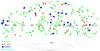 |
Fig. 1 Sky distribution of sources in our sample in J2000.0 coordinates. |
4.1. Total flux density
4.1.1. Total luminosity
Figures 2 and 3 show the 86 and 229 GHz luminosity ( , where dL is the luminosity distance2) as a function of redshift in our sample. A significant fraction of sources (51% [22%]) show 86 GHz flux densities below the 1 Jy (0.5 Jy) threshold, whereas only a small subset of eight sources (4%) shows S86> 5 Jy. At 229 GHz, 80% (48%) of the sources show flux densities below 1 Jy (0.5 Jy), and only 6 of them (3%) are brighter than 5 Jy. As expected, cosmologically distant quasars show the largest luminosities with a median
  W/Hz (
 W/Hz), followed by BL Lac objects with
  W/Hz (
 W/Hz), and radio galaxies
  W/Hz (
 W/Hz). This is consistent with expectations from the AGN unification theory (Urry & Padovani 1995), where quasars and BL Lacs are the relativistically Doppler boosted (i.e., beamed) versions of high power and low power radio galaxies (with their jets oriented closer to the plane of the sky), respectively.
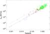 |
Fig. 2 86 GHz luminosity as a function of redshift. The dashed line indicates the luminosity for the observer’s frame flux density S86 = 0.5 Jy, whereas the dotted line is for S86 = 5 Jy. As for other figures hereafter, diamonds symbolize quasars, triangles denote BL Lacs, and squares are radio galaxies. |
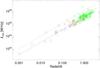 |
Fig. 3 229 GHz luminosity as a function of redshift. The dashed line indicates the luminosity for observer frame’s flux density S229 = 0.5 Jy, whereas the dotted line is for S229 = 5 Jy. |
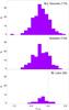 |
Fig. 4 Distribution of 15 GHz to 86 GHz spectral indices (α15, 86) for all sources in both the MOJAVE and our sample, and their corresponding quasar and BL Lac sub-samples. The 15 GHz total flux density was taken from integrated intensity of MOJAVE images. For each source, the 15 GHz observation taken at the closest date to our 86 GHz measurement was selected. Numbers in parentheses denote sample sizes. |
4.1.2. Spectral index
To study the spectral differences between quasars and BL Lacs, we determined the 15 to 86 GHz spectral index3 (α15,86) of quasars and BL Lacs. For that, we used the 15 GHz total flux densities from integrated intensities in available MOJAVE VLBA images4 with observations performed as contemporaneous as possible to our millimeter observations.
Similar to what it was found in Agudo et al. (2010), Fig. 4 shows that the α15, 86 spectral indices for both quasars and BL Lacs are distributed toward flat and optically thin spectral indices (with α15, 86 median  for quasars and
  for BL Lacs). Only a small fraction of sources (19% of quasars and 15% of BL Lacs) show α15, 86> 0. The smallest average spectral index of quasars with regard to that of BL Lacs is consistent with the well-known trend for BL Lacs to distribute the peaks of their synchrotron spectral energy distributions toward higher frequencies than quasars (e.g., Ackermann et al. 2011; Giommi et al. 2013). We also attribute part of the differences in spectral index between quasars and BL Lacs to the larger cosmological redshifts of quasars that shifts their spectra to lower frequencies in the observer’s frame.
The 86 to 229 spectral index distribution (α86, 229, see Fig. 5) also shows a similar trend with BL Lacs distributed toward slightly smaller spectral indexes with regard to quasars, although both the quasar and the BL Lac samples are distributed toward significantly smaller (more optically thin) spectral indexes (with  for quasars and
  for BL Lacs) for the case of α86, 229. These values are consistent with those for optically thin synchrotron radiation from AGN jets (Rybicki & Lightman 1979), which shows that blazars display optically thin radiation between 86 and 229 GHz in general and also guarantees that our polarimetric observations were not significantly affected by polarization angle rotation and depolarization owing to opacity effects. There are, however, a few exceptions, in particular 21 out of 180, for which the spectral index is flat or optically thick (with α86, 229 ≳ 0.25), perhaps, because of ongoing prominent flaring states (e.g., Marscher & Gear 1985).
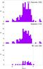 |
Fig. 5 Distribution of 86 GHz to 229 GHz spectral indices (α86, 229) for all sources detected at both frequencies in our sample. |
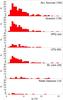 |
Fig. 6 Distribution of 86 GHz fractional linear polarization (red areas) for all sources in the sample, quasars, high optical polarization quasars (HPQ), low optical polarization quasars (LPQ), BL Lacs, and radio galaxies from top to bottom. N is the number of sources in 0.5% wide bins. Non-filled areas also include non-detection upper limits. Since we chose 3σ upper limits with a mean |

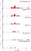 |
Fig. 7 Same as Fig. 6 but for 229 GHz fractional linear polarization. Since we chose 3σ upper limits with mean |

4.2. Linear polarization
Fractional linear polarization at 86 GHz (mL,86) was detected at ≥3σ level for 183 sources; this is 88% of the entire sample detected in total flux at 86 GHz (Fig. 6). At 229 GHz, the reduced sensitivity of our observations only allowed us to detect 23 sources. This corresponds to a 13% of all 181 sources detected at 229 GHz in total flux (Fig. 7).
We find the median values of mL, 86 for BL Lacs ( %) to be appreciably larger than those for quasars (
 %). A similar result is found for the 229 GHz linear polarization degree, where (
 %) is also much larger than for quasars (
 %). To make these comparisons, 3σ upper limits of values of mL were considered for non-detections of linear polarization to avoid overestimating the median of mL. The difference in the BL Lac and the quasar distributions of the linear polarization degree is confirmed by Gehan’s generalized Wilcoxon (GGW) test5 at 97.1% confidence level6 for the 86 distributions. Although the same test at 229 GHz gives a 99.9% confidence that the BL Lac and quasar distributions are different, this result should be taken with care given the low number statistics at this frequency. This result (i.e., quasars significantly less polarized than BL Lacs at millimeter wavelengths) was already pointed out at 86 GHz in Agudo et al. (2010).
The differences in the linear polarization degree of quasars and BL Lacs cannot be explained by differences in opacity in these two classes of sources, since we have already shown that both of them are in general optically thin between 86 and 229 GHz for most sources in their corresponding samples. Hovatta et al. (2009) and Pushkarev et al. (2009) suggested that quasars have, in general, smaller viewing angles than BL Lacs. The lower polarization degree of quasars with regard of BL Lacs that we report agree with these two studies. If quasars have smaller viewing angles than BL Lacs, the former should be affected by stronger depolarization along the line of sight. This requires the assumption that the magnetic fields in the jets of both quasars and BL Lacs are not homogeneously distributed along the jet axis or that their jets themselves are not axisymmetric.
In Agudo et al. (2010), we pointed out an apparent dichotomy in the 86 GHz distribution of the linear polarization degree of our entire source sample, which showed a peak at mL, 86 ≈ 2.5% and a second one at mL, 86 ≈ 4%. This behavior was also found at lower polarization degrees by Lister & Homan (2005) for the cores of quasars and the integrated polarization degree of EGRET-detected blazars. The data from our new survey further confirms the dichotomy found in Agudo et al. (2010). The mL, 86 distribution of the entire source sample (top panel of Fig. 6) also shows a hint of this dichotomy with the first peak in the range mL, 86 ∈ [1.5,2.5]%, and the second one at mL, 86 ≈ 4%. The lack of enough polarization sensitivity of our 229 GHz observations with regard to those at 86 GHz prevents us from studying this dichotomy at 229 GHz, where linear polarization below the 5% level is not detected (Fig. 7).
The similarity of the 86 GHz mL, 86 distributions of the entire source sample and that of quasars (that, however, only has a confidence of 78.9% according to our GGW test) might indicate that this dichotomy is produced by quasars but not by BL Lacs. Indeed, the mL, 86 distribution of BL Lacs is significantly different than those of quasars, see above. Here, we test the hypothesis that the bimodal mL, 86 is produced by high optical polarization quasars (HPQ, for the high polarization peak in the mL, 86 distribution of quasars) as listed in Véron-Cetty & Véron (2006) and low optical polarization quasars (LPQ, for the low polarization peak). This, however, does not seem to be a reliable explanation, given that the HPQ mL, 86 distribution is not clearly accumulated toward large linear polarization degrees, and we do not have the means to statistically demonstrate that the HPQ and LPQ mL distributions are significantly different (the GGW test gives only a 52.6% confidence for that). Therefore, although we have been able to confirm the dichotomy in the mL, 86 distribution of our entire source sample (quasars in particular), our new data remain inconclusive about the possible physical meaning of this apparent dichotomy.
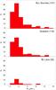 |
Fig. 8 Distribution of 86 GHz to 15 GHz fractional linear polarization ratio for sources with detected linear polarization in both our survey and MOJAVE. Six sources in the range 10 <mL, 86/mL, 15< 19 are not shown. The 15 GHz linear polarization fraction was computed from measurements of integrated total flux density and linearly polarized flux density from 15 GHz VLBI images taken by the MOJAVE team on the closest available dates to our 86 GHz observations. |
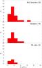 |
Fig. 9 Distribution of 229 GHz to 86 GHz fractional linear polarization ratio for sources with detected linear polarization at both frequencies (i.e., mL, 229/mL, 86). |
4.2.1. Fractional linear polarization ratio along the radio and millimeter spectrum
The linear polarization detection rate in our survey is ~ 88% at 86 GHz and ~ 13% at 229 GHz (see above). The 3σ level of linear polarization detection has medians of  % at 86 GHz and
  % at 229 GHz. Therefore, ~ 88% of our sources detected in total flux at 86 GHz show mL, 86 ≳ 1.0%, and ~ 13% of those detected in total flux at 229 GHz show mL, 229 ≳ 6.0%.
In contrast, 71% of the sources in both the MOJAVE and in our sample of 86 GHz detections show mL, 86 ≳ 1.0%, whereas only 8% of MOJAVE sources with linear polarization detected at 229 GHz display mL, 229 ≳ 6.0%. This points out a progressive increasing dependence of the fractional linear polarization of blazars with observing frequency (see also Agudo et al. 2006, 2010; Jorstad et al. 2007). This can also be discerned from Figs. 6 and 7.
By using the data from our first 3.5 AGN Polarimetric Survey in Agudo et al. (2010), we demonstrated that the 86 GHz linear polarization degree of blazars was, in general, around twice that at 15 GHz. Figure 8, where we plot the distributions of mL, 86/mL, 15 for those sources detected at 86 GHz in our survey and also with available contemporaneous 15 GHz MOJAVE measurements of the linear polarization degree, also show the same result. The entire source sample, quasars, and BL Lacs show significantly larger fractional linear polarization at 86 GHz than at 15 GHz by a mean factor ≈2 (Fig. 8). Essentially, the same result is found for the distributions of mL, 229/mL, 86, when the linear polarization of sources detected at 229 GHz in our survey is compared with their corresponding, simultaneously measured, 86 GHz linear polarization degree (Fig. 9). The median values of the mL, 86/mL, 15 and mL, 229/mL, 86 distributions show, however, slightly smaller values: 1.6, 1.6, and 1.5 for the entire sample, quasars, and BL Lacs, respectively, for the case of mL, 86/mL, 15 and 1.7, 1.7, and 1.5 for mL, 229/mL, 86.
Although there are some apparent differences in the different distributions shown in Figs. 8 and 9, our Kolmogorov–Smirnov (K-S) tests do not give a sufficiently high confidence to conclude that the quasar and BL Lac distributions of mL, 86/mL, 15 and mL, 229/mL, 86 are selected from different parent distributions (confidence level only 40.9%, and 88.3%, respectively). Note that there is also a prominent 18% (9%) fraction of sources with mL, 86/mL, 15 (mL, 229/mL, 86) ratio greater than 4. Such a tail of large, high-frequency linear-polarization excess seems to be present in both quasars and BL Lacs, although BL Lacs do not show it so clearly in mL, 229/mL, 86, perhaps, because of the lower number of sources in that sub-sample.
To explain the observed excess of mL, 86 with regard to mL, 15 by a factor of 2 (Agudo et al. 2010), we proposed two complementary explanations for this effect: a) that the 86 GHz emission in blazars comes from a region with a better ordered magnetic field than the 15 GHz one; and b) that the 15 GHz emission from blazars is affected by a considerably greater Faraday depolarization relative to the 86 GHz emission. Now that we have also studied the properties of the mL, 229/mL, 86 distributions in this work, we can safely assume that explanation b) is not reliable, at least for the comparison of the 86 and the 229 GHz emission, which is very unlikely to show appreciable Faraday rotations for a significant number of sources in our samples (see Sects. 1 and 4.3). Option a), along with the existing evidence that higher millimeter emission from blazars comes from inner regions upstream in their jets (e.g., Jorstad et al. 2007), imply that the magnetic field is progressively better ordered in blazar jet regions that are located progressively upstream in the jet.
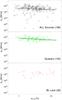 |
Fig. 10 86 GHz luminosity versus fractional linear polarization at 86 GHz for sources with known redshift for the entire source sample, quasars, and BL Lacs (from top to bottom). Arrows symbolize mL upper limits. The continuous lines symbolize the result of linear regressions. Numbers in parentheses denote sample sizes. |
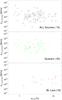 |
Fig. 11 Same as Fig. 10 but for unbeamed 86 GHz luminosities computed from Doppler factors given in Hovatta et al. (2009). |
4.2.2. Total luminosity vs. linear polarization
In Agudo et al. (2010), we reported a significant anti-correlation for the first time between the 86 GHz luminosity (L86) and the mL, 86 distribution for blazars in our previous 3.5 mm AGN Polarization Survey. The data from our new survey also reproduces such anti-correlation. Figure 10 shows L86 versus mL, 86 for sources with a known redshift in the entire source sample, quasars, and BL Lacs. Our Spearman’s ρ test for correlation gives ρ = −0.22 with a 99.7% confidence for the entire source sample and ρ = −0.27 with 99.9% confidence for quasars. Possibly because of the soft dependence of L86 versus mL, 86 and also because of the small number of measurements for BL Lacs, this anti–correlation cannot be confirmed for BL Lacs, for which ρ = 0.25 with 74.5% confidence. A similar analysis performed through the Generalized Spearman’s ρ test, made by using the ASURV 1.2 package by Lavalley et al. (1992), that takes into account both detections and upper limits, also points out statistically significant anti-correlation for quasars with ρ = −0.27 at 99.9% confidence. The Generalized Spearman’s ρ test only gives 91.2% confidence for ρ = −0.12 for the entire source sample when upper limits are accounted for, and even less (ρ = 0.24 at 76.9% confidence) for BL Lacs. At 229 GHz, the small number of linear polarization detections do not allow for reliable correlation studies of L229 versus mL, 229.
The confirmation of this result implies that the magnetic field order in jets of blazars increases with decreasing millimeter luminosity. In Agudo et al. (2010), we tested the hypothesis that the L versus mL anti-correlation would be only produced by orientation and relativistic effects; that is, the sources whose jets are better oriented to the line of sight are expected to display larger luminosities (because of their larger Doppler boosting) and also lower linear polarization degrees (because of cancellation of orthogonal polarization components along the line of sight). This was tested by computing the unbeamed luminosities (L86, unbeamed) of sources with known Doppler factors from Hovatta et al. (2009), but this hypothesis was ruled out. This is because a significant correlation was still found for a single sub-sample of sources. We have repeated the same test with our updated data set, and we have obtained no correlation between the Lunbeamed and mL (Fig. 11) for neither the entire source sample, quasars, nor BL Lacs. This opens again the possibility to use orientation and relativistic effects to explain the reported Lbeamed versus mL anti-correlation, although other alternative explanations (e.g., Agudo et al. 2010) cannot be ruled out.
4.2.3. Linear polarization angle vs. jet position angle
Figure 12 shows the distribution of misalignment of the jet position angle (φjet, see Table 1) with the polarization (electric vector) position angle at 86 GHz (χ86, see Table 2), this is, | χ86 − φjet |, for the entire source sample, quasars, and BL Lacs. To give the most reliable estimate of φjet as possible to compare it with our millimeter polarimetric measurements, we first searched in the 86 GHz VLBI Survey by Lee et al. (2008) and then followed it by the 15 GHz data from the MOJAVE survey (Lister & Homan 2005, preferentially). A more exhaustive search from references 1 to 10 in Table 1 was done for every source not found in these two surveys. If a source was found in several references, we adopted the higher frequency φjet measurement.
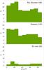 |
Fig. 12 Distribution of misalignment between χ86 and φjet. From top to bottom, we present, the entire source sample, the quasar, and the BL Lac sub-samples. |
Figure 12 shows a very weak (almost non-existent) trend for sources in our entire sample and quasars to distribute χ86 nearly parallel to φjet with 0° ≤ | χ86 − φjet | ≲ 30°. A similar result was also shown in Agudo et al. (2010). BL Lacs seem to show a different | χ86 − φjet | distribution, although also with an additional (but also very weak) excess of sources, where χ86 is almost parallel to φjet. However, our Kolmogorov-Smirnov (K-S) tests give a too weak confidence on the hypothesis that our entire source sample and quasars come from a different parent distribution than BL Lacs (12% and 23%, respectively). Therefore, it is not possible to confirm this difference. Our 229 GHz linear polarization angle measurements give similar results (Fig. 13). We also report a very weak trend for the 229 GHz polarization angle to distribute nearly parallel to the jet position angle for the entire source sample and quasars. The K-S test on their | χ229 − φjet | distributions give a 99.5% confidence to come from the same parent distribution. For BL Lacs, | χ229 − φjet | might be distributed in all possible misalignment angles, although the small number of sources in this case (Fig. 13) do not allow us to make any reliable statement or statistical tests.
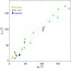 |
Fig. 14 86 GHz linear polarization angle (χ86) as compared to the simultaneously measured 229 GHz linear polarization angle (χ229) for the 22 sources with detected polarization at both 86 and 229 GHz. The dashed line represents the χ86 = χ229 line. |
Even for the case of the entire source sample considered for the | χ86 − φjet | histogram, the excess of sources accumulated toward 0° ≤ | χ86 − φjet | ≲ 30° only represents 17% of the total number of sources in our entire sample, which gives an idea of the small relevance of this excess. Therefore, we fully confirm that there is no clear trend for the millimeter linear polarization angle to be aligned either parallel or perpendicular to φjet for all source sub-samples considered here. This result contradicts theoretical expectations for purely axisymmetric jets, which predict that the polarization angle should be observed either parallel or perpendicular to the jet axis (e.g., Lyutikov et al. 2005; Cawthorne 2006). Moreover, several previous observational attempts to probe this bi-modality through observations at centimeter wavelengths (e.g., Gabuzda et al. 2000; Pollack et al. 2003; Lister & Homan 2005) do not agree among each other (see Agudo et al. 2010,for a summary on their differences).
There are three possible explanations for why our observations do not match the expectations from theory, namely, why we do not detect a clear trend of either quasars or BL Lacs to distribute their short millimeter polarization degree either parallel or perpendicular to the jet. These explanations are as follows: a) a larger χ variability amplitude and/or time scale at millimeter wavelengths with regard to those at longer centimeter wavelengths; b) different physical properties of the region where the bulk of the short millimeter emission is radiated (with regard to those at longer centimeter wavelengths); c) and significant departures from axisymmetric jet geometries and dynamics on the short millimeter emission regions that should show different expected integrated polarization angles than those for axisymmetric jets. Combinations of options a, b, and c are, of course, possible as well.
4.3. Faraday rotation between 86 and 229 GHz
In Fig. 14, we compare the linear polarization angle measured at 86 and 229 GHz for the 22 sources detected in polarization at both frequencies. The figure clearly shows that there is a general good match between χ86 and χ229 within the errors. Although there are some deviations from the χ86 = χ229 line in Fig. 14, none of the points are away from this line at more than 3σ with regard to the χ229 measurement. The relatively large χ229 uncertainties, which are typically several times larger than those at 86 GHz, do not allow us to provide a >3σ measurement of Faraday rotation measure (RM)7 for any of the sources with both 86 and 229 GHz polarization angle measurements. Instead, only a 3σ RM value, which is typically of the order of several times 104 rad m2, is given in Table 2 for the 22 sources mentioned above. This result is consistent with previous expectations for rotation measures not much larger than RM ~ 104 rad m-2, although we cannot rule out such large values with the available data. Large rotation measures have already been detected in some sources through ultra-high-resolution and high-precision polarimetric-VLBI observations (e.g., Attridge et al. 2005; Gómez et al. 2008, 2011; Agudo et al. 2012a).
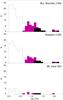 |
Fig. 15 Distribution of the absolute value of 86 GHz circular polarization for the entire source sample, quasars, and BL Lacs. Black areas correspond to mC, 86 detections at ≥3σ. Violet shaded areas indicate observing results with ≥2σ, whereas unshaded areas symbolize all mC measurements, regardless of their significance. |
5. Circular polarization
In Fig. 15, we present the distribution of the absolute value of 86 GHz circular polarization | mC,86 | for the samples considered here. We show the distributions of | mC,86 | detections at ≥3σ level (black), | mC,86 | measurements at ≥2σ level (violet), and all | mC,86 | measurements regardless of their significance (unshaded areas).
As expected from the previously known low level of circular polarization degree of blazars (typically ≲0.5% at 2 cm Homan & Lister 2006), we only detect mC,86 for a small fraction of sources (6%). This small detection rate is consistent with the one reported by Homan & Lister (2006) through 15 GHz VLBA observations (~ 15%), and our own results for our previous survey (Agudo et al. 2010), where we only detected circular polarization at 86 GHz for eight sources (6% of the entire sample). No circular polarization was detected from our 229 GHz observations.
Figure 15 shows that most of the 13 circular polarization detections correspond to values in the range 0.9% ≲ | mC, 86 | ≲ 1.6% (for sources 0229+131, 0430+052, 0451−282, 0716+714, 0917+449, 0954+658, 1324+224, 1328+307, 1642+690, 2131−021, and 2342−161), although there are two detections at | mC, 86 | ≈ 2% (for 0923+392 and 1124−186). These correspond to significantly larger | mC, 86 | values than those observed on our first survey (Agudo et al. 2010), where we only detected 86 GHz circular polarization in the range 0.3% ≲ | mC, 86 | ≲ 0.7%. Apart from variability, we do not have an explanation of why no large circular polarization values (| mC, 86 | ≳ 0.7%) were detected in our previous 86 GHz survey, although 8 sources detected in circular polarization in our new survey were also present in the sample of our previous survey.
Among all sources for which we detect 86 GHz circular polarization in our new survey, only one (1124−186 with mC, 86 = −1.98 ± 0.35%) was also detected in the previous survey (with mC, 86 = 0.58 ± 0.19%). We invoke circular polarization variability to explain this mC, 86 sign reversal and the large difference in | mC, 86 | between the observations of the two surveys in five years. This is consistent with circular polarization variability levels previously reported for radio-loud AGN (e.g., Aller et al. 2003).
Moreover, among all sources with detected mC, 86 in our new survey, only 0716+714 (with mC, 86 = −1.25 ± 0.35%) was also detected by the MOJAVE team with mC, 15 = + 0.37 ± 0.11%, which is also consistent with models that can reproduce considerable mC differences at different observing frequencies (e.g., Homan et al. 2009).
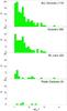 |
Fig. 16 Distribution of 86 GHz total flux variability ratio ( |
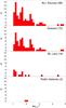 |
Fig. 17 Distribution of 86 GHz polarization degree variability ratio ( |
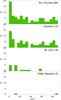 |
Fig. 18 Distribution of the absolute difference of the 86 GHz polarization angle in Agudo et al. (2010) and in this paper ( |
6. Total flux and linear polarization variability
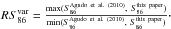
In Fig. 16, we compare the 86 GHz total flux density from the first 3.5 mm AGN Polarimetric Survey in Agudo et al. (2010) and the measurements presented in this paper using the 86 GHz total flux variability ratio ( )8. The figure clearly shows a large level of variability by a median factor of ~1.5 for the entire source sample at time scales ≲5 years and with 19% of sources displaying S86 variations by a factor >2. No significant difference in the distribution is found between any of the different samples considered in Fig. 16.
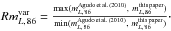
The distribution of the 86 GHz polarization degree variability ratio ( )9 is shown in Fig. 17. This Figure also points out an even larger degree of variability of mL, 86 with a median variability factor
  and with 34% of the sources displaying an increased (or decreased) mL, 86 by a factor of 2 on the time scale of years. We obtain similar results for the different sub-samples considered in Fig. 17. Note that and are not correlated (Spearman’s ρ = 0.17 with 21.1% confidence), hence reflecting the complicated time dependent behavior of different blazars studied in detail (e.g., Marscher et al. 2010; Jorstad et al. 2010; Agudo et al. 2011a,b; Wehrle et al. 2012).
The 86 GHz linear polarization angle is also highly variable on the time scale of years, as shown by Fig. 18, where we present the distribution of the absolute difference for the 86 GHz polarization angle from Agudo et al. (2010) and ( )10 for the entire source sample, quasars, BL Lacs, and radio galaxies in this paper. Figure 18 also shows that the difference of 86 GHz linear polarization angle of blazars on the time scale of years is essentially evenly distributed among all possible angles between 0° and 90°, except for a small fraction (14%) of sources that tend to conserve the same polarization angle in such time scales. There is a 90.2% probability for the quasar and the BL Lac distributions in Fig. 18 to come from different parent distributions, but this is not enough for us to claim a statistically significant difference between them with regard to the behavior of their polarization angle variability.
Radio-loud AGN, and blazars, in particular, are able to show extreme total flux density variability in the millimeter range (and in other spectral ranges) by up to one order of magnitude on a time scale from months (Jorstad et al. 2005; Teräsranta et al. 2005; Fuhrmann et al. 2008) to days (Agudo et al. 2006). Such extreme variability (enhanced by relativistic Doppler boosting) is often connected to the ejection and propagation of strong jet perturbations (blobs or shocks) from the innermost regions of the source (e.g., Jorstad et al. 2005, 2010; Kadler et al. 2008; Perucho et al. 2008; Marscher et al. 2010; Agudo et al. 2011a,b). Regarding linear polarization variability at short millimeter wavelengths, blazars have been shown to display mL excursions up to one order of magnitude and χ rotations that are >90° on time scales of months or even weeks (e.g. Jorstad et al. 2005, 2010; D’Arcangelo et al. 2007, 2009; Agudo et al. 2011a,b). It is thus not surprising that a large level of variability affects our results and, of course, the completeness of our sample (see Sect. 2). The expected influence of such variability in our study is to broaden the S, mL, and χ distributions or to hide their correlation with other variables – hence, making it more difficult to obtain statistically significant relations – but never faking results to give unrealistic correlations. We are therefore confident on the significance of the results shown here.
7. Summary
We have presented the first simultaneous 3.5 and 1.3 mm polarization survey of radio-loud AGN on a large sample of 211 sources, which are dominated by blazars.
Our total flux measurements show that almost all measured sources (96%) have a spectral index  . Most of them have an optically thin spectrum, between 86 and 229 GHz with median spectral indexes for quasars and for BL Lacs. In contrast, the 15 to 86 GHz spectral index is distributed toward flatter and mild optically-thin spectral indices for both quasars and BL Lacs.
We detect a linear polarization above 3σ levels for 88% and 13% of the sources detected at 86 and 229 GHz, respectively. We find that the median linear polarization degrees of quasars and BL Lacs are different at 86 GHz and 229 GHz: % and  % for quasars and % and
  % for BL Lacs. The difference between the quasar and BL Lac mL distributions at 86 GHz is significant to a 97.1% confidence level. This difference is consistent with recent work suggesting that quasars have, in general, smaller viewing angles than BL Lacs. This follows the assumption that the magnetic fields in the jets of BL Lacs and quasars are not homogeneously distributed along the jet axis or that the jets themselves are not axisymmetric.
We show for the first time that the 229 GHz linear polarization degree is in general a factor ~ 1.6 larger than the one at 86 GHz. We also confirm that the 86 GHz polarization degree is stronger than that at 15 GHz by a factor of ~ 1.6. We observed a good match between the measured polarization angles at 86 and 229 GHz for 22 sources. Therefore, at these wavelengths, it is unlikely to expect significant Faraday depolarization effects. As a result, the stronger linear polarization degree at higher frequencies suggests that the magnetic field is progressively better ordered in blazar jet regions that are located progressively upstream in the jet.
An anti-correlation between the millimeter luminosity and the linear polarization degree is confirmed here for the entire source sample and quasars at 86 GHz. We attribute this relation to purely relativistic and orientation effects. That is, sources whose jets are better oriented to the line of sight display larger luminosities (because of their larger Doppler boosting) and also lower linear polarization degrees (because orthogonal polarization components are cancelled along the line of sight).
Unlike theoretical predictions from axially symmetric jet models, we show an essentially non-existent relation between χ86 and the jet structural position angle for both quasars and BL Lacs for distributing at a preferential misalignment angle (see also Agudo et al. 2010). Only a small 17% of quasars tend to have 0° ≤ | χ86 − φjet | ≲ 30°. This result seems to be reproduced also at 229 GHz, although the small number of sources detected in polarization at this frequency do not allow us to obtain robust conclusions. These results imply that either the magnetic field or the emitting particle distributions (or both) that are responsible for the synchrotron radiation in the innermost regions where the short mm emission is radiated in blazars, have a markedly non axisymmetric character in general.
Comparison of our data with the 86 GHz measurements presented in Agudo et al. (2010) shows a considerable high total flux variability factor () with median variations of  on the time scale of years, where a 19% of sources show
  and even one source (0422+004) experiences extreme total flux variations by
  . The 86 GHz linear polarization degree is also equally highly variable with a median variability factor
  and with 34% of the sources displaying
  with maximum variations by a factor of ~ 5. The 86 GHz linear polarization angle is also highly variable on the time scale of years. Except for a small fraction (14%) of sources that tend to conserve the same polarization angle, most sources show drastically different polarization angles that are evenly distributed among all possible angles between 0° and 90° at such time scales.
Online material
Source properties.
Summary of observing results.
Note that the S90 GHz WMAP fluxes were estimated from extrapolation from the WMAP spectra and spectrum S60 GHz where a S90 GHz was not available.
We use hereafter a Ho = 71 km s-1 Mpc-1, Ωm = 0.27, and ΩΛ = 0.73 cosmology.
We define the spectral index between two observing frequencies ν1 and ν2 as αν1,ν2 = log (Sν1/Sν2)/log (ν1/ν2).
The Gehan’s generalized Wilcoxon test (Gehan 1965) considers both detections and upper limits. To perform our tests, we used the ASURV 1.2 survival analysis package (see Lavalley et al. 1992, and references therein).
Throughout this paper, only confidence levels ≥95.0% will be considered sufficiently high to claim that two distributions are significantly different.
RM = (χobs(λ) − χint) /λ2 with χint being the intrinsic polarization angle and χobs(λ) as the observed polarization angle at the observing wavelength λ.
Acknowledgments
The authors acknowledge the anonymous referee for his/her constructive revision of this paper, which allowed us to improve it considerably. This paper is based on observations carried out with the IRAM 30 m telescope. IRAM is supported by INSU/CNRS (France), MPG (Germany) and IGN (Spain). The research at the IAA-CSIC is supported in part by the Ministerio de Ciencia e Innovación of Spain, and by the regional government of Andalucía through grants AYA2010-14844 and P09-FQM-4784, respectively. The research at Boston University was funded by US National Science Foundation grant AST-0907893, NASA grants NNX08AJ64G, NNX08AU02G, NNX08AV61G, and NNX08AV65G, and NRAO award GSSP07-0009. This research has made use of the NASA/IPAC Extragalactic Database, the MOJAVE database (Lister et al. 2009), the one by the Blazar Research Group at the Boston University, as well as the USNO Radio Reference Frame Image Database.
References
- Ackermann, M., Ajello, M., Baldini, L., et al. 2010, ApJ, 721, 1383 [NASA ADS] [CrossRef] [Google Scholar]
- Ackermann, M., Ajello, M., Allafort, A., et al. 2011, ApJ, 743, 171 [NASA ADS] [CrossRef] [Google Scholar]
- Acosta-Pulido, J. A., Agudo, I., Barrena, R., et al. 2010, A&A, 519, A5 [NASA ADS] [CrossRef] [EDP Sciences] [Google Scholar]
- Agudo, I., Krichbaum, T. P., Ungerechts, H., et al. 2006, A&A, 456, 117 [NASA ADS] [CrossRef] [EDP Sciences] [Google Scholar]
- Agudo, I., Bach, U., Krichbaum, T. P., et al. 2007, A&A, 476, L17 [NASA ADS] [CrossRef] [EDP Sciences] [Google Scholar]
- Agudo, I., Thum, C., Wiesemeyer, H., & Krichbaum, T. P. 2010, ApJS, 189, 1 [NASA ADS] [CrossRef] [Google Scholar]
- Agudo, I., Jorstad, S. G., Marscher, A. P., et al. 2011a, ApJ, 726, L13 [NASA ADS] [CrossRef] [Google Scholar]
- Agudo, I., Marscher, A. P., Jorstad, S. G., et al. 2011b, ApJ, 735, L10 [NASA ADS] [CrossRef] [Google Scholar]
- Agudo, I., Gómez, J. L., Casadio, C., Cawthorne, T. V., & Roca-Sogorb, M. 2012a, ApJ, 752, 92 [NASA ADS] [CrossRef] [Google Scholar]
- Agudo, I., Marscher, A. P., Jorstad, S. G., et al. 2012b, ApJ, 747, 63 [CrossRef] [Google Scholar]
- Aller, H. D., Aller, M. F., & Plotkin, R. M. 2003, ApSS, 288, 17 [Google Scholar]
- Attridge, J. M., Wardle, J. F. C., & Homan, D. C. 2005, ApJ, 633, L85 [NASA ADS] [CrossRef] [Google Scholar]
- Bach, U., Villata, M., Raiteri, C. M., et al. 2006, A&A, 456, 105 [NASA ADS] [CrossRef] [EDP Sciences] [Google Scholar]
- Blandford, R. D., & Payne, D. G. 1982, MNRAS, 199, 883 [NASA ADS] [CrossRef] [Google Scholar]
- Carter, M., Lazareff, B., Maier, D., et al. 2012, A&A, 538, A89 [NASA ADS] [CrossRef] [EDP Sciences] [Google Scholar]
- Cawthorne, T. V. 2006, MNRAS, 367, 851 [NASA ADS] [CrossRef] [Google Scholar]
- Cohen, R. D., Smith, H. E., Junkkarinen, V. T., & Burbidge, E. M. 1987, ApJ, 318, 577 [NASA ADS] [CrossRef] [Google Scholar]
- D’Arcangelo, F. D., Marscher, A. P., Jorstad, S. G., et al. 2007, ApJ, 659, L107 [NASA ADS] [CrossRef] [Google Scholar]
- D’arcangelo, F. D., Marscher, A. P., Jorstad, S. G., et al. 2009, ApJ, 697, 985 [NASA ADS] [CrossRef] [Google Scholar]
- de Vaucouleurs, G., de Vaucouleurs, A., Corvin, H. G., et al. 1991, Third Reference Catalogue of Bright Galaxies. (New York: Springer) [Google Scholar]
- Fuhrmann, L., Krichbaum, T. P., Witzel, A., et al. 2008, A&A, 490, 1019 [NASA ADS] [CrossRef] [EDP Sciences] [Google Scholar]
- Gehan, E. A. 1965, Biometrika, 52, 203 [CrossRef] [Google Scholar]
- Gabuzda, D. C., Pushkarev, A. B., & Cawthorne, T. V. 2000, MNRAS, 319, 1109 [NASA ADS] [CrossRef] [Google Scholar]
- Giommi, P., Padovani, P., & Polenta, G. 2013, MNRAS, 431, 1914 [NASA ADS] [CrossRef] [Google Scholar]
- Gold, B., Odegard, N., Weiland, J. L., et al. 2011, ApJS, 192, 15 [Google Scholar]
- Gómez, J. L., Marscher, A. P., Alberdi, A., Jorstad, S. G., & Agudo, I. 2001, ApJ, 561, L161 [NASA ADS] [CrossRef] [Google Scholar]
- Gómez, J. L., Marscher, A. P., Jorstad, S. G., Agudo, I., & Roca-Sogorb, M. 2008, ApJ, 681, L69 [NASA ADS] [CrossRef] [Google Scholar]
- Gómez, J. L., Roca-Sogorb, M., Agudo, I., Marscher, A. P., & Jorstad, S. G. 2011, ApJ, 733, 11 [NASA ADS] [CrossRef] [Google Scholar]
- Healey, S. E., Romani, R. W., Cotter, G., et al. 2008, ApJS, 175, 97 [NASA ADS] [CrossRef] [Google Scholar]
- Homan, D. C., & Lister, M. L. 2006, AJ, 131, 1262 [NASA ADS] [CrossRef] [Google Scholar]
- Homan, D. C., Lister, M. L., Aller, H. D., Aller, M. F., & Wardle, J. F. C. 2009, ApJ, 696, 328 [NASA ADS] [CrossRef] [Google Scholar]
- Hovatta, T., Valtaoja, E., Tornikoski, M., & Lähteenmäki, A. 2009, A&A, 494, 527 [NASA ADS] [CrossRef] [EDP Sciences] [Google Scholar]
- Jorstad, S. G., Marscher, A. P., Lister, M. L., et al. 2005, AJ, 130, 1418 [NASA ADS] [CrossRef] [Google Scholar]
- Jorstad, S. G., Marscher, A. P., Stevens, J. A., et al. 2007, AJ, 134, 799 [NASA ADS] [CrossRef] [Google Scholar]
- Jorstad, S. G., Marscher, A. P., Larionov, V. M., et al. 2010, ApJ, 715, 362 [NASA ADS] [CrossRef] [Google Scholar]
- Kadler, M., Ros, E., Lobanov, A. P., Falcke, H., & Zensus, J. A. 2004, A&A, 426, 481 [NASA ADS] [CrossRef] [EDP Sciences] [Google Scholar]
- Kadler, M., Ros, E., Perucho, M., et al. 2008, ApJ, 680, 867 [NASA ADS] [CrossRef] [Google Scholar]
- Lavalley, M., Isobe, T., & Feigelson, E. 1992, in Astronomical Data Analysis Software and Systems I, eds. D. M. Worrall, C. Biemesderfer, & J. Barnes (ASP: San Francisco), ASP Conf. Ser., 25, 245 [Google Scholar]
- Lawrence, C. R., Pearson, T. J., Readhead, A. C. S., & Unwin, S. C. 1986, AJ, 91, 494 [NASA ADS] [CrossRef] [Google Scholar]
- Lee, S.-S., Lobanov, A. P., Krichbaum, T. P., et al. 2008, AJ, 136, 159 [NASA ADS] [CrossRef] [Google Scholar]
- Lister, M. L., & Homan, D. C. 2005, AJ, 130, 1389 [NASA ADS] [CrossRef] [Google Scholar]
- Lister, M. L., Aller, H. D., Aller, M. F., et al. 2009, AJ, 137, 3718 [NASA ADS] [CrossRef] [Google Scholar]
- Lyutikov, M., Pariev, V. I., & Gabuzda, D. C. 2005, MNRAS, 360, 869 [NASA ADS] [CrossRef] [Google Scholar]
- Marscher, A. P., & Gear, W. K. 1985, ApJ, 298, 114 [NASA ADS] [CrossRef] [Google Scholar]
- Marscher, A. P., Jorstad, S. G., Larionov, V. M., et al. 2010, ApJ, 710, L126 [NASA ADS] [CrossRef] [Google Scholar]
- Nilsson, K., Pursimo, T., Sillanpää, A., Takalo, L. O., & Lindfors, E. 2008, A&A, 487, L29 [NASA ADS] [CrossRef] [EDP Sciences] [Google Scholar]
- Perucho, M., Agudo, I., Gómez, J. L., et al. 2008, A&A, 489, L29 [NASA ADS] [CrossRef] [EDP Sciences] [Google Scholar]
- Pollack, L. K., Taylor, G. B., & Zavala, R. T. 2003, ApJ, 589, 733 [NASA ADS] [CrossRef] [Google Scholar]
- Pushkarev, A. B., Kovalev, Y. Y., Lister, M. L., & Savolainen, T. 2009, A&A, 507, L33 [NASA ADS] [CrossRef] [EDP Sciences] [Google Scholar]
- Rybicki, G. B., & Lightman, A. P. 1979, Rad. Process. Astrophys. (New York: Wiley Interscience) [Google Scholar]
- Sbarufatti, B., Treves, A., & Falomo, R. 2005, ApJ, 635, 173 [NASA ADS] [CrossRef] [Google Scholar]
- Sowards-Emmerd, D., Romani, R. W., Michelson, P. F., Healey, S. E., & Nolan, P. L. 2005, ApJ, 626, 95 [NASA ADS] [CrossRef] [Google Scholar]
- Tavecchio, F., Ghisellini, G., Bonnoli, G., & Ghirlanda, G. 2010, MNRAS, 405, L94 [NASA ADS] [CrossRef] [Google Scholar]
- Teräsranta, H., Wiren, S., Koivisto, P., Saarinen, V., & Hovatta, T. 2005, A&A, 440, 409 [NASA ADS] [CrossRef] [EDP Sciences] [Google Scholar]
- Thum, C., Wiesemeyer, H., Paubert, G., Navarro, S., & Morris, D. 2008, PASP, 120, 777 [NASA ADS] [CrossRef] [Google Scholar]
- Urry, C. M., & Padovani, P. 1995, PASP, 107, 803 [NASA ADS] [CrossRef] [Google Scholar]
- Véron-Cetty, M.-P., & Véron, P. 2006, A&A, 455, 773 [NASA ADS] [CrossRef] [EDP Sciences] [Google Scholar]
- Wehrle, A. E., Marscher, A. P., Jorstad, S. G., et al. 2012, ApJ, 758, 72 [NASA ADS] [CrossRef] [Google Scholar]
- Zavala, R. T., & Taylor, G. B. 2004, ApJ, 612, 749 [NASA ADS] [CrossRef] [Google Scholar]
All Tables
All Figures
|
Fig. 1 Sky distribution of sources in our sample in J2000.0 coordinates. |
| In the text | |
|
Fig. 2 86 GHz luminosity as a function of redshift. The dashed line indicates the luminosity for the observer’s frame flux density S86 = 0.5 Jy, whereas the dotted line is for S86 = 5 Jy. As for other figures hereafter, diamonds symbolize quasars, triangles denote BL Lacs, and squares are radio galaxies. |
| In the text | |
|
Fig. 3 229 GHz luminosity as a function of redshift. The dashed line indicates the luminosity for observer frame’s flux density S229 = 0.5 Jy, whereas the dotted line is for S229 = 5 Jy. |
| In the text | |
|
Fig. 4 Distribution of 15 GHz to 86 GHz spectral indices (α15, 86) for all sources in both the MOJAVE and our sample, and their corresponding quasar and BL Lac sub-samples. The 15 GHz total flux density was taken from integrated intensity of MOJAVE images. For each source, the 15 GHz observation taken at the closest date to our 86 GHz measurement was selected. Numbers in parentheses denote sample sizes. |
| In the text | |
|
Fig. 5 Distribution of 86 GHz to 229 GHz spectral indices (α86, 229) for all sources detected at both frequencies in our sample. |
| In the text | |
|
Fig. 6 Distribution of 86 GHz fractional linear polarization (red areas) for all sources in the sample, quasars, high optical polarization quasars (HPQ), low optical polarization quasars (LPQ), BL Lacs, and radio galaxies from top to bottom. N is the number of sources in 0.5% wide bins. Non-filled areas also include non-detection upper limits. Since we chose 3σ upper limits with a mean |
| In the text | |
|
Fig. 7 Same as Fig. 6 but for 229 GHz fractional linear polarization. Since we chose 3σ upper limits with mean |
| In the text | |
|
Fig. 8 Distribution of 86 GHz to 15 GHz fractional linear polarization ratio for sources with detected linear polarization in both our survey and MOJAVE. Six sources in the range 10 <mL, 86/mL, 15< 19 are not shown. The 15 GHz linear polarization fraction was computed from measurements of integrated total flux density and linearly polarized flux density from 15 GHz VLBI images taken by the MOJAVE team on the closest available dates to our 86 GHz observations. |
| In the text | |
|
Fig. 9 Distribution of 229 GHz to 86 GHz fractional linear polarization ratio for sources with detected linear polarization at both frequencies (i.e., mL, 229/mL, 86). |
| In the text | |
|
Fig. 10 86 GHz luminosity versus fractional linear polarization at 86 GHz for sources with known redshift for the entire source sample, quasars, and BL Lacs (from top to bottom). Arrows symbolize mL upper limits. The continuous lines symbolize the result of linear regressions. Numbers in parentheses denote sample sizes. |
| In the text | |
|
Fig. 11 Same as Fig. 10 but for unbeamed 86 GHz luminosities computed from Doppler factors given in Hovatta et al. (2009). |
| In the text | |
|
Fig. 12 Distribution of misalignment between χ86 and φjet. From top to bottom, we present, the entire source sample, the quasar, and the BL Lac sub-samples. |
| In the text | |
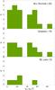 |
Fig. 13 Same as Fig. 12 but for 230 GHz linear polarization angle (χ230) measurements. |
| In the text | |
|
Fig. 14 86 GHz linear polarization angle (χ86) as compared to the simultaneously measured 229 GHz linear polarization angle (χ229) for the 22 sources with detected polarization at both 86 and 229 GHz. The dashed line represents the χ86 = χ229 line. |
| In the text | |
|
Fig. 15 Distribution of the absolute value of 86 GHz circular polarization for the entire source sample, quasars, and BL Lacs. Black areas correspond to mC, 86 detections at ≥3σ. Violet shaded areas indicate observing results with ≥2σ, whereas unshaded areas symbolize all mC measurements, regardless of their significance. |
| In the text | |
|
Fig. 16 Distribution of 86 GHz total flux variability ratio ( |
| In the text | |
|
Fig. 17 Distribution of 86 GHz polarization degree variability ratio ( |
| In the text | |
|
Fig. 18 Distribution of the absolute difference of the 86 GHz polarization angle in Agudo et al. (2010) and in this paper ( |
| In the text | |
Current usage metrics show cumulative count of Article Views (full-text article views including HTML views, PDF and ePub downloads, according to the available data) and Abstracts Views on Vision4Press platform.
Data correspond to usage on the plateform after 2015. The current usage metrics is available 48-96 hours after online publication and is updated daily on week days.
Initial download of the metrics may take a while.