© ESO, 2014

1. Introduction

Aperture-synthesis imaging in the infrared can provide us with unique insights into many types of astrophysical objects. However, image reconstruction from infrared interferograms is usually very challenging because of the small number of available telescopes, severe atmospheric wavefront degradation, short atmospheric coherence time, and photon and detector noise. In the last two decades, several image reconstruction algorithms were developed for aperture-synthesis imaging with infrared arrays. Examples include the BBM method (building block mapping; Hofmann & Weigelt 1993; Hofmann et al. 2005), BSMEM (bispectrum maximum entropy method; Buscher 1994), MIRA (multi-aperture image reconstruction algorithm; Thiebaut 2002), and MACIM (Monte-Carlo imaging; Ireland et al. 2006). The performance of various algorithms was evaluated in several blind tests (Lawson et al. 2004, 2006; Malbet et al. 2010; Baron et al. 2012) initiated by the IAU Working Group on Optical/IR Interferometry. In contrast to our BBM method, the new IRBis method (image reconstruction software using the bispectrum) employs a fast minimization routine based on conjugate gradients (Hager & Zhang 2005, 2006).

This paper is structured as follows. In Sect. 2, we describe the new IRBis software, and in Sect. 3, we present applications of the IRBis image reconstruction algorithm to computer-simulated interferograms.

2. IRBis image reconstruction software

The goal of infrared aperture-synthesis imaging is to reconstruct an image from the measured calibrated visibilities and closure phases of the target observed with an interferometer. The processing steps of IRBis in brief are:

• 1.

  The raw data of the image reconstruction process are the measured calibrated squared visibilities and closure phases at several positions in the uv plane. From these observations, the observed bispectrum elements (see Sect. 2.1) and their errors are computed. These bispectrum elements are the measured interferometric data set used to derive the image intensity distribution of the astronomical target observed.

• 2.

  The iterative IRBis algorithm searches for the k-th two-dimensional image o_k(x), whose bispectrum best agrees with the interferometrically observed bispectrum (x is a two-dimensional coordinate vector).

• 3.

  Because of the sparse uv coverage of present infrared interferometers, a regularization term H [o_k(x)] is added to the reduced χ² function Q [o_k(x)] of the interferometric data to obtain the cost function J [o_k(x)]. This regularization (see Sect. 2.2.2) is required to find a good reconstruction out of the many reconstructions with a good χ² value.

• 4.

  Minimization of the cost function J [o_k(x)] is performed by the large-scale, bound-constrained nonlinear optimization algorithm ASA_CG (Hager & Zhang 2005, 2006). The algorithm ASA_CG is a fast conjugate gradient based active set algorithm for solving large-scale bound-constrained nonlinear optimization problems with simple bounds on its variables.

2.1. Preparation of the interferometric data for image reconstruction

The input data for image reconstruction are the available calibrated object bispectrum elements, which are determined with the interferometer for a number of spatial frequency coordinates (f₁,f₂) of the object bispectrum given by 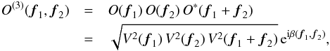$\begin{array}{ccc}{\mathit{O}}^{\mathrm{\left(}\mathrm{3}\mathrm{\right)}}\mathrm{\left(}{{f}}_{\mathrm{1}}\mathit{,}{{f}}_{\mathrm{2}}\mathrm{\right)}& \mathrm{=}& \mathit{O}\mathrm{\left(}{{f}}_{\mathrm{1}}\mathrm{\right)}\hspace{0.17em}\mathit{O}\mathrm{\left(}{{f}}_{\mathrm{2}}\mathrm{\right)}\hspace{0.17em}{\mathit{O}}^{\mathrm{\ast }}\mathrm{(}{{f}}_{\mathrm{1}}\mathrm{+}{{f}}_{\mathrm{2}}\mathrm{)}\\ & \mathrm{=}& \end{array}$(1)where O(f₁) and O(f₂) are the Fourier transforms of the target intensity distribution at the spatial frequency vectors f₁ and f₂, respectively, and O^∗(f₁ + f₂) is the conjugate complex of the target Fourier transform at coordinate f₁ + f₂. (Both f₁ and f₂ are two-dimensional spatial frequency vectors in Fourier space; that is, O⁽³⁾(f₁,f₂) is four-dimensional.) The object bispectrum O⁽³⁾(f₁,f₂) is formed using the measured squared visibilities V²(f₁) = | O(f₁) | ² and the measured closure phases β(f₁,f₂) (see Eq. (1)). The error σ_{O⁽³⁾(f1,f2)} of the bispectrum is calculated using the error of the bispectrum modulus σ_{| O⁽³⁾(f1,f2) |} and of the closure phase σ_β(f1,f2), as discussed in the Appendix A.

The spatial frequency vectors f₁ = u₁/λ and f₂ = u₂/λ are derived from the projected baseline vectors u₁ and u₂, respectively, and the wavelength λ of the interferometric data measured. Because the reconstructed image should lie in a squared field with a certain field-of-view (FOV) size and because this FOV is represented by a grid of n_pixel × n_pixel, the spatial frequencies f₁ have to be transformed to pixel coordinates 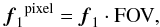${{{f}}_{\mathrm{1}}}^{\mathrm{pixel}}\mathrm{=}{{f}}_{\mathrm{1}}\mathrm{·}\mathrm{FOV}\mathit{,}$(2)where the units of FOV and f₁ are, for example, arcsec and arcsec^-1, respectively. Throughout the paper, f₁ and f₂ denote spatial frequencies, which are transformed to pixel coordinates according to Eq. (2).

Because the unequal distribution of the measured uv points in the uv plane may cause artifacts in the reconstructed image, the squared bispectrum residuals in the following equation can be weighted with a weight w_d(f₁,f₂) to partially compensate their unequal distribution in the calculation of the reduced χ²: 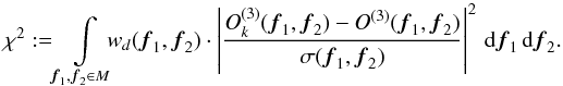${\mathit{\chi }}^{\mathrm{2}}\mathrm{:}\mathrm{=}\underset{}{{\mathrm{\int }}^{{{f}}_{\mathrm{1}}\mathit{,}{{f}}_{\mathrm{2}}\mathrm{\in }\mathit{M}}}{\mathit{w}}_{\mathit{d}}\mathrm{\left(}{{f}}_{\mathrm{1}}\mathit{,}{{f}}_{\mathrm{2}}\mathrm{\right)}\mathrm{·}{\left|\frac{{\mathit{O}}_{\mathit{k}}^{\mathrm{\left(}\mathrm{3}\mathrm{\right)}}\mathrm{\left(}{{f}}_{\mathrm{1}}\mathit{,}{{f}}_{\mathrm{2}}\mathrm{\right)}\mathrm{-}{\mathit{O}}^{\mathrm{\left(}\mathrm{3}\mathrm{\right)}}\mathrm{\left(}{{f}}_{\mathrm{1}}\mathit{,}{{f}}_{\mathrm{2}}\mathrm{\right)}}{\mathit{\sigma }\mathrm{\left(}{{f}}_{\mathrm{1}}\mathit{,}{{f}}_{\mathrm{2}}\mathrm{\right)}}\right|}^{\mathrm{2}}\hspace{0.17em}\mathrm{d}{{f}}_{\mathrm{1}}\hspace{0.17em}\mathrm{d}{{f}}_{\mathrm{2}}\mathit{.}$(3)The variable M denotes the set consisting of the spatial frequency coordinates (f₁,f₂) of all measured bispectrum elements O⁽³⁾(f₁,f₂) with their errors σ(f₁,f₂). The uv point density weight w_d(f₁,f₂) in the above equation can, for example, be chosen to be proportional to the inverse density of the spatial frequencies (f₁,f₂) ∈ M of the observed bispectrum elements, or can be chosen to be another function or a constant. The function w_d(f₁,f₂) is normalized with ${}^{\mathrm{\int }}\mathit{w}_{\mathit{d}}\mathrm{\left(}{{f}}_{\mathrm{1}}\mathit{,}{{f}}_{\mathrm{2}}\mathrm{\right)}\hspace{0.17em}\mathrm{d}{{f}}_{\mathrm{1}}\hspace{0.17em}\mathrm{d}{{f}}_{\mathrm{2}}\mathrm{=}\mathrm{1}$. The above equation shows that the total weight of the χ² function is w(f₁,f₂) = w_d(f₁,f₂) /σ²(f₁,f₂). For the calculation of the spatial frequency density, see Appendix B.

2.2. The cost function

2.2.1. Measurement term in the cost function

The goal of image reconstruction is to find the best target image that agrees with the interferometric data determined (bispectrum elements) within the error bars. To this end, the measured bispectrum elements have to be compared to the bispectrum of the actual image during the iterative reconstruction process. This comparison is performed using reduced χ² functions. In IRBis, two different functions Q₁ [o_k(x)] and Q₂ [o_k(x)] are offered for the cost function (see Eq. (6)). The function Q₁ [o_k(x)] is the χ² function of the bispectrum given by $\begin{array}{ccc}{\mathit{Q}}_{\mathrm{1}}\mathrm{\left[}{\mathit{o}}_{\mathit{k}}\mathrm{\right(}{x}\mathrm{\left)}\mathrm{\right]}& \mathrm{:}\mathrm{=}& \underset{}{{\mathrm{\int }}^{{{f}}_{\mathrm{1}}\mathit{,}{{f}}_{\mathrm{2}}\mathrm{\in }\mathit{M}}}\frac{{\mathit{w}}_{\mathit{d}}\mathrm{\left(}{{f}}_{\mathrm{1}}\mathit{,}{{f}}_{\mathrm{2}}\mathrm{\right)}}{{\mathit{\sigma }}^{\mathrm{2}}\mathrm{\left(}{{f}}_{\mathrm{1}}\mathit{,}{{f}}_{\mathrm{2}}\mathrm{\right)}}\mathrm{·}{\left|{\mathit{\gamma }}_{\mathrm{0}}\hspace{0.17em}{\mathit{O}}_{\mathit{k}}^{\mathrm{\left(}\mathrm{3}\mathrm{\right)}}\mathrm{\left(}{{f}}_{\mathrm{1}}\mathit{,}{{f}}_{\mathrm{2}}\mathrm{\right)}\mathrm{-}{\mathit{O}}^{\mathrm{\left(}\mathrm{3}\mathrm{\right)}}\mathrm{\left(}{{f}}_{\mathrm{1}}\mathit{,}{{f}}_{\mathrm{2}}\mathrm{\right)}\right|}^{\mathrm{2}}\hspace{0.17em}\\ & & \end{array}$(4)Here, o_k(x) is the instantaneous iterated image with its bispectrum elements ${\mathit{O}}_{\mathit{k}}^{\mathrm{\left(}\mathrm{3}\mathrm{\right)}}\mathrm{\left(}{{f}}_{\mathrm{1}}\mathit{,}{{f}}_{\mathrm{2}}\mathrm{\right)}$, M denotes the set consisting of the spatial frequency coordinates f₁,f₂ of all observed bispectrum elements O⁽³⁾(f₁,f₂). w_d(f₁,f₂) and σ(f₁,f₂) are the uv point denisty weights and errors of the observed bispectrum elements, respectively. Because o_k(x) is not normalized during the reconstruction procedure (and therefore ${\mathit{O}}_{\mathit{k}}^{\mathrm{\left(}\mathrm{3}\mathrm{\right)}}\mathrm{\left(}\mathrm{0}\mathit{,}\mathrm{0}\mathrm{\right)}\ne \mathrm{1}$), it is helpful to scale the bispectrum ${\mathit{O}}_{\mathit{k}}^{\mathrm{\left(}\mathrm{3}\mathrm{\right)}}\mathrm{\left(}{{f}}_{\mathrm{1}}\mathit{,}{{f}}_{\mathrm{2}}\mathrm{\right)}$ by a factor γ₀ so that the actual value of Q₁ [o_k(x)] is minimal.

The second alternative Q₂ [o_k(x)] is the χ² function of the bispectrum phasors given by $\begin{array}{ccc}& & {\mathit{Q}}_{\mathrm{2}}\mathrm{\left[}{\mathit{o}}_{\mathit{k}}\mathrm{\right(}{x}\mathrm{\left)}\mathrm{\right]}\mathrm{:}\mathrm{=}\\ & & \hspace{0.17em}\hspace{0.17em}\underset{}{{\mathrm{\int }}^{{{f}}_{\mathrm{1}}\mathit{,}{{f}}_{\mathrm{2}}\mathrm{\in }\mathit{M}}}\{\{\frac{{\mathit{w}}_{\mathit{d}}\mathrm{\left(}{{f}}_{\mathrm{1}}\mathit{,}{{f}}_{\mathrm{2}}\mathrm{\right)}}{{\mathit{\sigma }}_{\mathit{\beta }}^{\mathrm{2}}\mathrm{\left(}{{f}}_{\mathrm{1}}\mathit{,}{{f}}_{\mathrm{2}}\mathrm{\right)}}\mathrm{·}\mathrm{|}{\mathit{\gamma }}_{\mathrm{0}}\exp \mathrm{\left[}\mathrm{i}{\mathit{\beta }}_{\mathit{k}}\mathrm{\right(}{{f}}_{\mathrm{1}}\mathit{,}{{f}}_{\mathrm{2}}\mathrm{\left)}\mathrm{\right]}\mathrm{-}\exp \mathrm{\left[}\mathrm{i}\hspace{0.17em}\mathit{\beta }\mathrm{\right(}{{f}}_{\mathrm{1}}\mathit{,}{{f}}_{\mathrm{2}}\mathrm{\left)}\mathrm{\right]}{\mathrm{|}}^{\mathrm{2}}\\ & & \end{array}$(5)Here, β(f₁,f₂) and β_k(f₁,f₂) denote the measured closure phases and the closure phases in the current iterated image, respectively. The functions σ_β(f₁,f₂) and σ_m(f₁,f₂) are the errors of the bispectrum phasors and the bispectrum moduli, respectively. The factor γ₀ scales the bispectrum phasor and the bispectrum modulus of the iterated image to minimize the value of Q₂ [o_k(x)]. The variable f₀ is the relative weight between the closure phase term and the bispectrum modulus term in Q₂ [o_k(x)]. The variable f₀ can be determined by image reconstruction tests. The f₀ value providing the best χ² is chosen. The function Q₂ [o_k(x)] is more sensitive to the closure phases than Q₁ [o_k(x)], because it does not weight the bispectrum phasor down with the bispectrum modulus as in Q₁ [o_k(x)]. Note that the modulus term in the above equation consists of the triple product of the measured visibilities that include the squared visibilities, which lie on the axes of the bispectrum (e.g., O⁽³⁾(f₁,f₂ = 0) = | O(f₁) | ²). Because the spatial frequencies of the measurements, which are transformed to the pixel coordinates according to Eq. (2), usually do not lie exactly on the pixel grid, the Fourier transform of the iterated image o_k(x) is linearly interpolated at the spatial frequencies f₁, f₂ and −f₁ − f₂ to create the bispectrum element ${\mathit{O}}_{\mathit{k}}^{\mathrm{\left(}\mathrm{3}\mathrm{\right)}}\mathrm{\left(}{{f}}_{\mathrm{1}}\mathit{,}{{f}}_{\mathrm{2}}\mathrm{\right)}$.

2.2.2. Regularization term in the cost function

Because of the sparse uv coverage and noise, many different reconstructed images with very small values of the Q₁ [o_k(x)] or Q₂ [o_k(x)] function may exist. For example, within holes of the sparse uv coverage, strange Fourier values of an iterated image (for example, rapidly changing values instead of smoothly changing values) could appear, leading to reconstructions with strong artifacts. To avoid such artifacts in the reconstruction, some prior information, as, for example, the smoothness of the target, its limited extent, its positivity, etc. has to be given to the reconstruction process. Therefore, the image reconstruction algorithm has to search for the image that agrees with both the interferometric measurements and the prior information about the target. Regularization is introduced to the reconstruction process in two different ways: (a) regularization utilizing the limited extent of the target by limiting the reconstruction area to the area of a binary circular mask; and (b) regularization forcing the smoothness of the reconstruction when a regularization function H [o_k(x)] to the Q₁ [o_k(x)] or Q₂ [o_k(x)] function of the actual reconstruction (Wahl 1984; Cornwell 1983) is added. Therefore, the algorithm searches for the image o_k(x) (within the area of the binary circular mask) that minimizes the cost function $\mathit{J}\mathrm{\left[}{\mathit{o}}_{\mathit{k}}\mathrm{\right(}{x}\mathrm{\left)}\mathrm{\right]}\mathrm{:}\mathrm{=}\mathit{Q}\mathrm{\left[}{\mathit{o}}_{\mathit{k}}\mathrm{\right(}{x}\mathrm{\left)}\mathrm{\right]}\mathrm{+}\mathit{\mu }\mathrm{·}\mathit{H}\mathrm{\left[}{\mathit{o}}_{\mathit{k}}\mathrm{\right(}{x}\mathrm{\left)}\mathrm{\right]}\mathit{,}$(6)where μ is the regularization parameter or Langrange parameter defining the strength of the influence of the regularization function H [o_k(x)]. In the IRBis, the following regularization functions are currently implemented:

1) The “pixel intensity” quadratic:

regularization function (Tikhonov) enforcing compactness of the reconstruction, which is given by $\mathit{H}\mathrm{\left[}{\mathit{o}}_{\mathit{k}}\mathrm{\right(}{x}\mathrm{\left)}\mathrm{\right]}\mathrm{:}\mathrm{=}\mathrm{\int }\frac{{\mathit{o}}_{\mathit{k}}\mathrm{(}{x}{\mathrm{)}}^{\mathrm{2}}}{\mathrm{prior}\mathrm{\left(}{x}\mathrm{\right)}}\hspace{0.17em}\mathrm{d}{x}\mathit{.}$(7)In this paper, it is called RG1.

2) The Maximum Entropy:

regularization function (Narayan & Nityananda 1986) is given by $\mathit{H}\mathrm{\left[}{\mathit{o}}_{\mathit{k}}\mathrm{\right(}{x}\mathrm{\left)}\mathrm{\right]}\mathrm{:}\mathrm{=}\mathrm{\int }\left\{{\mathit{o}}_{\mathit{k}}\mathrm{\left(}{x}\mathrm{\right)}\mathrm{·}\log \left\{\frac{{\mathit{o}}_{\mathit{k}}\mathrm{\left(}{x}\mathrm{\right)}}{\mathrm{prior}\mathrm{\left(}{x}\mathrm{\right)}}\right\}\mathrm{-}{\mathit{o}}_{\mathit{k}}\mathrm{\left(}{x}\mathrm{\right)}\mathrm{+}\mathrm{prior}\mathrm{\left(}{x}\mathrm{\right)}\right\}\mathrm{d}{x}\mathit{,}$(8)where prior(x) is a rough estimate of the target image, for example, a Gaussian or uniform disk fitted to the interferometric data. In this paper, it is called RG2.

3) The “pixel difference” quadratic:

regularization function, which enforces smoothness of the reconstruction because it has a minimum for small pixel intensity differences, is given by $\begin{array}{ccc}\mathit{H}\mathrm{\left[}{\mathit{o}}_{\mathit{k}}\mathrm{\right(}{x}\mathrm{\left)}\mathrm{\right]}\mathrm{:}\mathrm{=}& & \\ \mathrm{\int }\frac{\mathrm{\left|}{\mathit{o}}_{\mathit{k}}\mathrm{\right(}{x}\mathrm{)}\mathrm{-}{\mathit{o}}_{\mathit{k}}\mathrm{(}{x}\mathrm{+}\mathrm{\Delta }{x}\mathrm{)}{\mathrm{|}}^{\mathrm{2}}\mathrm{+}\mathrm{|}{\mathit{o}}_{\mathit{k}}\mathrm{\left(}{x}\mathrm{\right)}\mathrm{-}{\mathit{o}}_{\mathit{k}}\mathrm{(}{x}\mathrm{+}\mathrm{\Delta }{y}\mathrm{)}{\mathrm{|}}^{\mathrm{2}}}{\mathrm{prior}\mathrm{\left(}{x}\mathrm{\right)}}\hspace{0.17em}\mathrm{d}{x}& & \end{array}$(9)with shift vectors Δx = (1,0) and Δy = (0,1). In this paper, it is called RG3.

4) The edge preserving:

regularization function (Teboul et al. 1998) is given by $\begin{array}{ccc}& & \mathit{H}\mathrm{\left[}{\mathit{o}}_{\mathit{k}}\mathrm{\right(}{x}\mathrm{\left)}\mathrm{\right]}\mathrm{:}\mathrm{=}\\ & & \mathrm{\int }\frac{\sqrt{\mathrm{\left|}{\mathit{o}}_{\mathit{k}}\mathrm{\right(}{x}\mathrm{)}\mathrm{-}{\mathit{o}}_{\mathit{k}}\mathrm{(}{x}\mathrm{+}\mathrm{\Delta }{x}\mathrm{)}{\mathrm{|}}^{\mathrm{2}}\mathrm{+}\mathrm{|}{\mathit{o}}_{\mathit{k}}\mathrm{\left(}{x}\mathrm{\right)}\mathrm{-}{\mathit{o}}_{\mathit{k}}\mathrm{(}{x}\mathrm{+}\mathrm{\Delta }{y}\mathrm{)}{\mathrm{|}}^{\mathrm{2}}\mathrm{+}{\mathit{ϵ}}^{\mathrm{2}}}\mathrm{-}\mathit{ϵ}}{\mathrm{prior}\mathrm{\left(}{x}\mathrm{\right)}}\hspace{0.17em}\mathrm{d}{x}\mathit{,}\end{array}$(10)with the shift vectors Δx = (1,0) and Δy = (0,1). If ϵ² ≫ [ | o_k(x) − o_k(x + Δx) | ² + | o_k(x) − o_k(x + Δy) | ²], then H [o_k(x)] is nearly identical to the above “pixel difference” quadratic regularization function (Eq. (9)), which enforces smoothness of the reconstruction. On the other hand, if ϵ² ≪ [ | o_k(x) − o_k(x + Δx) | ² + | o_k(x) − o_k(x + Δy) | ²], then H [o_k(x)] is identical to the total variation (Rudin et al. 1992) regularization function preserving important details, such as edges. In this paper, it is called RG4. With a regularization prior prior(x) of constant intensity distribution, it is called RG4b.

All regularization functions presented above enforce smoothness in the image plane. Smoothness in the Fourier plane is also important to avoid unphysical fluctuations of the Fourier transform of the image caused by the sparse uv coverage of present optical/infrared long-baseline interferometers. Smoothness in the Fourier plane can be achieved by allowing reconstructed image intensity distributions within a small area in the image plane only. This limitation is introduced by binary masks. The built-in binary masks are circular with a defined radius. The size or radius of the mask can be, for example, chosen a little bit larger than the target size and can be estimated by a fit to the measured squared visibilities.

2.3. The minimization routine

The minimization of the cost function J [o_k(x)] can be performed by large-scale, bound-constrained nonlinear optimization algorithms. They are called large-scale because of the huge number of image pixels in the reconstruction: o_k(x) is considered to be an ~10⁴ − 10⁵ dimensional vector with its intensity values as coordinates. It is bound-constrained because of the positivity of the reconstruction and the normalization of its integral to one and is nonlinear because of the nonlinearity of the cost function (e.g., the χ² function of the bispectrum).

The image reconstruction software presented in this paper uses the nonlinear optimization algorithm ASA_CG (Hager & Zhang 2006). The algorithm ASA_CG is a conjugate gradient based active set algorithm for solving large-scale, bound-constrained, nonlinear optimization problems with simple bounds on its variables. The algorithm ASA_CG consists of a nonmonotone gradient projection step, an unconstrained optimization step, and a set of rules for branching between the two steps. The algorithm ASA_CG utilizes the cyclic Barzilai-Borwein algorithm (Dai et al. 2006) for the gradient projection step and the conjugate gradient algorithm CG_DESCENT (Hager & Zhang 2005) for the unconstrained optimization step.

The variables in the image reconstruction problem are the pixel intensities o_k(x). The simple bounds on the variables are the positive pixel intensities (o_k(x) > 0; positivity constraint). The input data for the minimization routine are the cost function J [o_k(x)] and its first derivatives, according to the pixel intensities o_k(x₀); that is, $\frac{\mathit{\partial J}\mathrm{\left[}{\mathit{o}}_{\mathit{k}}\mathrm{\right(}{x}\mathrm{\left)}\mathrm{\right]}}{\mathit{\partial }{\mathit{o}}_{\mathit{k}}\mathrm{\left(}{{x}}_{\mathrm{0}}\mathrm{\right)}}\mathrm{=}\frac{\mathit{\partial Q}\mathrm{\left[}{\mathit{o}}_{\mathit{k}}\mathrm{\right(}{x}\mathrm{\left)}\mathrm{\right]}}{\mathit{\partial }{\mathit{o}}_{\mathit{k}}\mathrm{\left(}{{x}}_{\mathrm{0}}\mathrm{\right)}}\mathrm{+}\mathit{\mu }\mathrm{·}\frac{\mathit{\partial H}\mathrm{\left[}{\mathit{o}}_{\mathit{k}}\mathrm{\right(}{x}\mathrm{\left)}\mathrm{\right]}}{\mathit{\partial }{\mathit{o}}_{\mathit{k}}\mathrm{\left(}{{x}}_{\mathrm{0}}\mathrm{\right)}}\mathit{,}$(11)where Q [o_k(x)] stands for one of the two χ² functions Q₁ [o_k(x)] and Q₂ [o_k(x)] as described in Eqs. (4) and (5). The minimization algorithm stops if the length of the gradient of the cost function is close to zero – that is, if it is smaller than a given small positive number. Starting images are, for example, a Gaussian, a uniform disk, or any other model function with sizes that are estimated by a fit to the measured interferometric data of the target.

2.4. Quality estimate of the reconstruction

The quality of the reconstructed image is estimated (a) by calculating the reduced χ² of the measured squared visibilities and closure phases (${\mathit{\chi }}_{{\mathit{V}}^{\mathrm{2}}}^{\mathrm{2}}$, ${\mathit{\chi }}_{\mathrm{CP}}^{\mathrm{2}}$) and (b) by calculating their residual ratios (ρρ_V², ρρ_CP). The residual ratio is the ratio between the sum of all positive residuals and the sum of all negative residuals of the squared visibilities and closure phases, respectively. Computer experiments show that the fit is good if the positive and negative residuals are equally distributed (i.e., if the residual ratio is close to one). For example, the residual ratio ρρ_CP of the closure phases is given by $\mathit{\rho }{\mathit{\rho }}_{\mathrm{CP}}\mathrm{:}\mathrm{=}\frac{\underset{}{{\mathrm{\int }}^{{{f}}_{\mathrm{1}}\mathit{,}{{f}}_{\mathrm{2}}\mathrm{\in }{\mathit{M}}_{\mathrm{+}}}}\mathrm{\left[}{\mathit{\beta }}_{\mathit{k}}\mathrm{\right(}{{f}}_{\mathrm{1}}\mathit{,}{{f}}_{\mathrm{2}}\mathrm{)}\mathrm{-}\mathit{\beta }\mathrm{(}{{f}}_{\mathrm{1}}\mathit{,}{{f}}_{\mathrm{2}}\mathrm{\left)}\mathrm{\right]}\mathit{/}{\mathit{\sigma }}_{\mathit{\beta }\mathrm{\left(}{{f}}_{\mathrm{1}}\mathit{,}{{f}}_{\mathrm{2}}\mathrm{\right)}}\hspace{0.17em}\mathrm{d}{{f}}_{\mathrm{1}}\mathrm{d}{{f}}_{\mathrm{2}}}{\underset{}{{\mathrm{\int }}^{{{f}}_{\mathrm{1}}\mathit{,}{{f}}_{\mathrm{2}}\mathrm{\in }{\mathit{M}}_{\mathrm{-}}}}\mathrm{\left[}{\mathit{\beta }}_{\mathit{k}}\mathrm{\right(}{{f}}_{\mathrm{1}}\mathit{,}{{f}}_{\mathrm{2}}\mathrm{)}\mathrm{-}\mathit{\beta }\mathrm{(}{{f}}_{\mathrm{1}}\mathit{,}{{f}}_{\mathrm{2}}\mathrm{\left)}\mathrm{\right]}\mathit{/}{\mathit{\sigma }}_{\mathit{\beta }\mathrm{\left(}{{f}}_{\mathrm{1}}\mathit{,}{{f}}_{\mathrm{2}}\mathrm{\right)}}\hspace{0.17em}\mathrm{d}{{f}}_{\mathrm{1}}\mathrm{d}{{f}}_{\mathrm{2}}}\mathit{,}$(12)where M₊ (M₋) denotes the collection of all measured closure phases at spatial frequency pairs (f₁,f₂) with positive (negative) residuals [β_k(f₁,f₂) − β(f₁,f₂)] /σ_β(f1,f2).

Because the reconstructed image is a good fit to the data if the reduced χ² values and the residual ratios are close to one, the quality of the reconstruction is measured by the positive parameter ${\mathit{q}}_{\mathrm{rec}}\mathrm{:}\mathrm{=}\mathrm{1}\mathit{/}\mathrm{4}\mathrm{·}\mathrm{\left[}\mathrm{\right|}{\mathit{\chi }}_{{\mathit{V}}^{\mathrm{2}}}^{\mathrm{2}}\mathrm{-}\mathrm{1}\mathrm{|}\mathrm{+}\mathrm{|}\mathit{\rho }{\mathit{\rho }}_{{\mathit{V}}^{\mathrm{2}}}\mathrm{-}\mathrm{1}\mathrm{|}\mathrm{+}\mathrm{|}{\mathit{\chi }}_{\mathrm{CP}}^{\mathrm{2}}\mathrm{-}\mathrm{1}\mathrm{|}\mathrm{+}\mathrm{|}\mathit{\rho }{\mathit{\rho }}_{\mathrm{CP}}\mathrm{-}\mathrm{1}\mathrm{\left|}\mathrm{\right]}\mathit{.}$(13)Therefore, a good reconstruction should have q_rec values close to zero. Note that q_rec defined in this way does recognize very well, if there are χ² and ρρ values much bigger than one. However, this definition of q_rec does not recognize the presence of noise fitting well, which occurs if χ² or ρρ values are close to zero. Therefore, to avoid noise fitting, the inverse 1 /χ² is used instead of χ² in Eq. (13) if the χ² value is smaller than one. The same procedure is applied to the ρρ values.

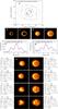Fig. 1 Computer simulation of aperture-synthesis imaging with the IRBis image reconstruction method: a) uv coverage (see Table 1); b), c) intensity distribution of the two different disk-star computer targets (diameter 11.2 and 16.8 mas) (central star is clippped for display); d), e) intensity distribution of the targets convolved with the point spread function (PSF) of the simulated interferometer; f), g) examples of simulated interferograms (total number of interferograms is 250 per uv point) with 1219 and 573 photons per interferogram and simulated additive detector read-out noise (RON) of 10 electrons (the average value of the RON is subtracted); h) reconstructed images of the two targets for 10 e− RON and different photon numbers ⟨ N ⟩ per interferogram (from 1219 to 152). For each reconstruction, the labels give the corresponding average photon number ⟨ N ⟩ per interferogram, V2 S/N, CP error, χ2 function (Q1, Q2), regularization function (RG1, RG2, RG3, RG4, RG4b), χ2, residual ratio ρρ, and the restoration error ρ (see text).

2.5. Processing scheme of the presented image reconstruction algorithm

The main reconstruction parameters of the presented IRBis image reconstruction algorithm are the radius of the binary circular image mask and the strength of the regularization parameters μ (see Sect. 2.2.2). To find a good reconstruction, the algorithm computes many reconstructions using several different radii of the binary image mask and several different regularization parameters during the image reconstruction run. Typically, a value of n = 6 different image mask radii and m = 6 different regularization parameters are chosen. Then the images for all combinations of image mask radii and regularization parameters are calculated.

The computation run with n different image mask radii is called the image mask radius run. The computation run with one fixed image mask radius (within the image mask radius run) and with m different regularization parameters is called a regularization parameter run in the following text.

Furthermore, an input start image and input regularization prior (see Sect. 2.2.2) has to be chosen. Possible choices are fits of simple models (e.g., Gaussian, uniform disk, etc.) to the interferometric data. The possible choices for start images and regularization priors are as follows for the image mask radius run and the regularization parameter run.

• 1.

  Possible choices for the start image and the regularization prior in each image mask radius run are:

  • (a)

    the input start image (explained above; e.g., Gaussian fit), denoted by Rs1, and the input regularization prior (explained above; e.g., Gaussian fit), denoted by Rp1, or

  • (b)

    the best reconstruction from the image mask radius run before, denoted by Rs2 (for the start image) and denoted by Rp2 (for the regularization prior), or

  • (c)

    the best reconstruction in this image reconstruction run so far, denoted by Rs3 (for the start image) and denoted by Rp3 (for the regularization prior).

• 2.

  Possible choices for the start image and the regularization priorin each regularization parameter run are:

  • (a)

    the selected start image of the current image mask radius run(i.e., Rs1, Rs2, or Rs3), denoted by Ms1, and the selectedregularization prior of the current image mask radius run (i.e.,Rp1, Rp2, or Rp3), denoted by Mp1, or

  • (b)

    the reconstruction from the preceding regularization parameter run, denoted by Ms2 (for the start image) and denoted by Mp2 (for the regularization prior), or

  • (c)

    the best reconstruction from the current image mask radius run, denoted by Ms3 (for the start image) and denoted by Mp3 (for the regularization prior).

A complete image reconstruction run consists of several image mask radius runs and regularization parameter runs, which are described above. That is, within each image reconstruction run, many images with different binary circular image masks and different regularization parameters are reconstructed. During the image reconstruction run, the quality of the reconstructions is measured with the parameter q_rec, as defined in Eq. (13). Many experiments with computer-simulated data show that it is a good choice to use the image reconstructed in the run before (i.e., choice (b), corresponding to options Rs2, Rp2, Ms2, and Mp2 as described above) as a start image and regularization prior of the current reconstruction. This approach quickly converges to the correct image. Of course, the strength of the regularization parameters has to be chosen properly. This is checked by reconstruction tests. In the following computer experiments (Sects. 3.1 and 3.2), choice (b) (i.e., the options Rs2, Rp2, Ms2, and Mp2 described above) was applied. Choices (a) and (c) seem to be not as efficient as choice (b) in most tests with simulated data. These alternatives will be investigated in a future paper in detail.

The following list summarizes the basic inputs of the algorithm:

• 1.

  the measured visibilities and closure phases of the target;

• 2.

  a start and a prior image, such as a Gaussian, uniform disk, etc. fitted to the measured visibilities;

• 3.

  the size of the FOV of the reconstruction;

• 4.

  the selection of one of the two χ² functions Q [o_k(x)] defined in Eqs. (4) and (5);

• 5.

  the selection of one regularization function H [o_k(x)] out of those presented in Eqs. (7)–(10);

• 6.

  the start image mask radius, the step size for changing its radius, and the number of steps (the new image mask radius is the current one plus the step size);

• 7.

  the start value of the regularization parameter μ, the factor to change it for the next test, and the number of regularization parameter tests;

• 8.

  the selection of the start image and the regularization prior for the next image mask radius run, which include the options Rs1, Rs2, or Rs3, and Rp1, Rp2, or Rp3, respectively;

• 9.

  the selection of the start image and the regularization prior for the next regularization parameter run, which include the options Ms1, Ms2, or Ms3, and Mp1, Mp2, or Mp3, respectively.

During an image reconstruction run, a large number of reconstructions are performed, and the reconstruction with the lowest value of the parameter q_rec is chosen as the final outcome. The above described image reconstruction parameters, which include the initial start radius of the circular binary mask, the step size to change it, the initial value of the regularization parameter μ, the factor to change it, and the number of changes, have to be defined by the user. The initial start radius can, for example, be estimated by fitting a simple model (e.g., a Gaussian, uniform disk, etc.) to the measured visibilities. The values of the initial regularization parameter and the factor to change it can be estimated by the user with image reconstruction tests. The criteria to estimate these parameter values are based on goodness-of-fit metrics (i.e., the q_rec parameter).

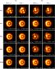Fig. 2 Dependence of the reconstructions on (a) the regularization functions H [ok(x)] used and (b) the χ2 function Q [ok(x)] applied in the cost function. This study shows reconstructions of the 16.8 mas disk-star target obtained in the experiment, as shown in Fig. 1 (for average S/N ~ 9 of the squared visibilities). Each row presents the reconstructions performed with one of the five regularization functions (RG1, RG2, RG3, RG4, and RG4b; see text and Eqs. (7)–(10)). The first two columns are reconstructions using the χ2 function Q1 [ok(x)] (see Eq. (4)) and the last two columns are reconstructions with the χ2 function Q2 [ok(x)] (see Eq. (5)). The columns labeled with “best qrec” are the reconstructions with the smallest value of qrec and those labeled with “best ρ” are the reconstructions with the smallest distance to the theoretical target. In each image, its restoration error ρ and its value of the reconstruction quality parameter qrec is presented.

3. Applications of the IRBis method to computer-simulated interferometric data

In this section, we describe several image reconstruction studies using the IRBis method. We also present the IRBis reconstructions submitted to the 2012 imaging beauty contest (Baron et al. 2012).

3.1. IRBis image reconstruction experiments with computer-simulated interferograms

Computer simulations of interferometric image reconstruction are a powerful tool for investigating the reliability of image reconstruction in the presence of severe noise and poor uv coverage. The comparison of the known target with the image reconstructed from the computer-simulated interferograms allows us to accurately measure the quality of the reconstruction. In astronomical applications, this is usually not possible because the intensity distribution of the target is usually not known. The raw data of such computer simulations can be, for example, (1) a set of visibilities and closure phases of a target or (2) a large number of individual target interferograms, as in this paper. In both cases, realistic noise has to be injected to the data.

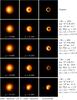Fig. 3 Same image reconstruction experiments as in Fig. 1 but with three different angular resolutions: (left column) resolution λ/D, or standard diffraction-limited resolution obtained by convolving the IRBis reconstruction with the diffraction-limited PSF of the interferometer, (middle column) resolution λ/2D (super-resolution), and (right column) IRBis reconstruction without convolving the original IRBis reconstruction with a PSF (i.e., some smoothing is only caused by regularization). The original synthetic target (diameter = 5.6 mas; see Table 2 for more details) is shown at the top with resolutions λ/D, λ/2D, and without any convolution (from left to right). For each reconstruction, the same information labels as in Fig. 1 are given. See text for more details.

Data simulation:

in the computer simulations presented in Figs. 1−3, we simulated the individual interferograms (see examples in Figs. 1f and g.) and a uv coverage (Fig. 1a) that corresponds to AMBER observations with the ATs (auxillary telescopes) of the ESO Very Large Telescope Interferometer (VLTI). The uv coverage in Fig. 1a corresponds to the conditions listed in Table 1. In the computer simulations presented in Figs. 1−3, we simulated 250 different interferograms per uv point. We used three different synthetic targets, which consist of a ring-like disk and a central star (with diameters of 5.6, 11.2, and 16.8 mas). The parameters of these simple targets are described in Table 2 in more detail. The interferometric diffraction-limited resolution λ/D (D = longest projected baseline) of the chosen array is 5.0 mas (D = 82.5 m, λ = 2.0 μm). The interferograms were simulated as if they were observed with a 3-telescope beam combiner. For each of the three baselines of each triangle telescope configuration, a spatial fringe pattern (i.e., a multiaxial 2-telescope interferogram in image space) was computed. Figures 1f and g show two examples of the computer-simulated interferograms.

The interferograms were degraded by various amounts of photon and detector noise with a read-out noise of 10 electrons (RON; typical for near-infrared Hawaii detectors). For each of the three baselines of all closure triplets listed in Table 1, 250 two-telescope interferograms were generated. The average power spectra and bispectra were calculated from the interferograms. After subtracting the noise bias terms, the calibrated visibilities, closure phases, and bispectrum elements were derived.

Image reconstruction:

Fig. 1 shows the image reconstruction results obtained with two different asymmetric ring-like disks with a central star. From top to bottom, we show the uv coverage (Fig. 1a), the two synthetic disk-star targets (Figs. 1b and c), the targets convolved with the diffraction-limited interferometer point spead function (Figs. 1d and e), two different example interferograms (Figs. 1f and g), and the reconstructed images derived for different amounts of simulated noise (Fig. 1h). In all computer experiments, we simulated a RON of ten electons. The simulated photon noise increases from top to bottom in Fig. 1h. The average number of photons ⟨ N ⟩ per interferogram is given for each of the eight reconstructed images in the information labels with several other image reconstruction parameters. The different average photon numbers ⟨ N ⟩ lead to different S/N of the squared visibilities and closure phase errors, which are also listed for each reconstructed image. The following parameters were used to reconstruct the images shown in Figs. 1−3. The input start image and the input regularization prior were a fully darkened circular disk fitted to the measured visibilities. The reconstructions were performed within a FOV of 100 mas. The bispectrum χ² function Q₁ [o_k(x)] (Eq. (4)) and the bispectrum phasor χ² function Q₂ [o_k(x)] with f₀ = 10 (f₀ is the relative weight between the bispectrum phasor and modulus term, as seen in Eq. (5).) were applied as the χ² function. The regularization functions used were the “pixel intensity” quadratic (RG1, see Eq. (7)), the “maximum entropy” (RG2, see Eq. (8)), the “pixel difference” quadratic (RG3, see Eq. (9)), and the “edge preserving” (RG4 and RG4b with ϵ = 1.0, see Eq. (10)) functions. The start image mask radius, the step size, and the number of steps were as follows: 5 mas, 3 mas, and 12, respectively, for the 11.2 mas disk-star system (Fig. 1b); 10 mas, 3 mas, and 12, respectively, for the 16.8 mas disk-star system (Fig. 1c); and 10 mas, 3 mas, and 12, respectively, for the 5.6 mas disk-star system (Fig. 3 top). For all targets, the start values of the regularization parameter μ were 2.0, 1.0, and 0.5; the factor to change it for the next test was 0.1, and the number of regularization parameter tests was 10. The best reconstruction from the last image mask radius run, which is Rs2 and Rp2, was applied as the start image and regularization prior for the next image mask radius run. The reconstruction from the last regularization parameter run, which is Ms2 and Mp2, was used as the start image and regularization prior for the next regularization parameter run.

For each target and noise level, 15 reconstructions were obtained from 15 image reconstruction runs. Each image reconstruction run is one of the 15 combinations of the five different regularization functions (i.e., RG1, RG2, RG3, RG4, and RG4b) and the three different start values of the regularization parameter (i.e., μ = 2.0, 1.0, and 0.5). The reconstructed image obtained from one image reconstruction run is the image (out of the set of all images produced) that has the smallest value of the reconstruction quality parameter q_rec (Eq. (13)). Each reconstruction presented in Figs. 1 and 3 is that reconstruction (obtained from the 15 image reconstruction runs), which has the smallest value of q_rec. These reconstructions are the best reconstructions out of the set of all 15 reconstructions obtained with each of the five different regularization methods and three different start values of the regularization parameter. These many image reconstruction runs have to be performed because it is not known which parameter choice is the best for a given data set. The quality parameter q_rec was used to find the best image of each image reconstruction run. The reconstructions were performed on standard PCs, and each of the 15 image reconstruction runs (consisting of twelve image mask radius runs and ten regularization parameter runs, which gives a total of 120 reconstruction runs) lasted about 5 to 10 min.

Figure 1h shows the dependence of the quality of the reconstructed image on the noise in the data. The reconstructions of the two disk-star computer targets with diameters of 11.2 mas and 16.8 mas, which are obtained from the data with average V² S/N values of ~20 and 9, are of good quality (i.e., restoration errors ρ = 0.060–0.104). The reconstructions from data with average V² S/N values of ~4 and 2 are of poor quality (i.e., restoration errors ρ = 0.179–0.365).

Figures 1 and 3 also present the restoration error ρ of each reconstruction. The restoration error is defined as 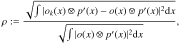$\mathit{\rho }\mathrm{:}\mathrm{=}\frac{\sqrt{\mathrm{\int }\mathrm{\left|}{\mathit{o}}_{\mathit{k}}\mathrm{\right(}\mathit{x}\mathrm{)}\mathrm{\otimes }{\mathit{p}}^{\mathrm{\prime }}\mathrm{(}\mathit{x}\mathrm{)}\mathrm{-}\mathit{o}\mathrm{(}\mathit{x}\mathrm{)}\mathrm{\otimes }{\mathit{p}}^{\mathrm{\prime }}\mathrm{(}\mathit{x}\mathrm{)}{\mathrm{|}}^{\mathrm{2}}\mathrm{d}\mathit{x}}}{\sqrt{\mathrm{\int }\mathrm{\left|}\mathit{o}\mathrm{\right(}\mathit{x}\mathrm{)}\mathrm{\otimes }{\mathit{p}}^{\mathrm{\prime }}\mathrm{(}\mathit{x}\mathrm{)}{\mathrm{|}}^{\mathrm{2}}\mathrm{d}\mathit{x}}}\mathit{,}$(14)where o(x) ⊗ p′(x) and o_k(x) ⊗ p′(x) are the original object and reconstruction, respectively, convolved with the same point spread function (PSF) p′(x). The PSF p′(x) is the diffraction-limited interferometer PSF (diameter = λ/longest projected baseline) or a smaller PSF in the case of super-resolution experiments). In Figs. 1–3, the restoration error ρ is measured within a FOV of 100 mas.

Figure 2 presents the dependence of the reconstructed images on (a) the regularization function used (i.e., RG1, RG2, RG3, RG4, or RG4b in Eqs. (7)–(10)) and (b) the χ² function (Q₁ [o_k(x)] or Q₂ [o_k(x)], see Eqs. (4) and (5)) applied in the cost function. This study is performed with the 16.8 mas disk-star target and for an average S/N~ 9 of the squared visibilities (shown in Fig. 1). For this target, S/N, and uv coverage, the χ² function Q₁ [o_k(x)] yields the best reconstructions. With Q₁ [o_k(x)], all regularization functions, except RG1, yield reconstructions of similar good quality, that is, ρ = 0.104 to 0.124. The best result is obtained with RG2 (“maximum entropy”, ρ = 0.104).

In Fig. 3, we compare reconstructions calculated with the standard diffraction-limited interferometer resolution λ/D (D = longest baseline) obtained by convolving the original IRBis reconstruction with the diffraction-limited PSF of the interferometer with (1) the reconstruction calculated with the higher resolution λ/2D and (2) the original IRBis reconstruction (That is, reconstruction without any convolution; regularization is the only smoothing in this case.). The goal of this study is to investigate whether the resolution can be increased (i.e., whether so-called super-resolution is possible) if the S/N of the raw data is very high. The compact disk-star target has a diameter of 5.6 mas (see Table 2). The image reconstruction procedure was the same as described for Fig. 1. The labels in Fig. 3 give the same information as in Fig. 1. The reconstructions in Fig. 3 demonstrate that slightly higher angular resolution than the standard resolution (λ/D) can be obtained if the S/N of the observations is high enough. For example, with 2× interferometer resolution (λ/2D), the hole in the ring and the brighter left part of the ring can be recognized (except at lowest S/N with average V²S/N = 4.7). These features are not visibile in the case of the standard interferometer resolution (λ/D). However, pushing the resolution in this way to higher values is dangerous in actual astronomical observations, because this resolution enhancement is essentially an extrapolation of the observed Fourier data to higher spatial frequencies and therefore very sensitive to systematic errors of the data at high spatial frequencies.

3.2. IRBis reconstructions submitted to the 2012 imaging beauty contest

In this section, we describe the IRBis image reconstruction steps of the submitted beauty contest reconstructions in more detail than in Baron et al. (2012). At the time of the 2012 imaging beauty contest, we used another name, namely IRS, for the applied IRBis method.

For the 2012 imaging beauty contest, two different targets were used, a synthetic T Tauri star-disk system and a red supergiant target with bright spots. The T Tauri system was modeled using the TORUS 3D (Harries 2011) radiative transfer code. The T Tauri system consists of an unresolved central star, an inclined disk with a diameter of roughly 3.5 mas, and a bias (background) intensity within a square of ~6 mas size. The red supergiant has a diameter of about ~4.0 mas. The original targets were not known at the time of the imaging beauty contest (blind test) before the submission deadline for the colleagues who submitted their reconstructions. The interferometric data of both targets were simulated as if they were observed with the 6-telescope beam combiner MIRC-6T (Monnier et al. 2010) at the CHARA Array (ten Brummelaar et al. 2005) atop Mt. Wilson. The data were simulated with eight spectral channels in the H band, and it was assumed that both targets have wavelength-independent intensity distributions. The uv coverage of the T Tauri system corresponds to five hours of observing time with observations acquired every fifteen minutes. The uv coverage of the red supergiant was directly copied from previous AZ Cyg observations. The top panels of Figs. 4 and 5 show the simulated uv coverage of the T Tauri system and the red supergiant, respectively. The simulated visibilities and closure phases were degraded by realistic noise and not derived from individual, noise-degraded interferograms as in the previous section. For the T Tauri system, the empirical noise model for MIRC-6T was applied yielding a very low signal-to-noise ratio (average S/N of the V² data ~2.3, average closure phase error ~38°), and for the red supergiant, noise amplitudes derived from previous AZ Cyg observations were applied (average S/N of the V² data ~4.2, average closure phase error ~20°).

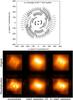Fig. 4 IRBis aperture-synthesis imaging of a synthetic T Tauri star-disk system submitted to the 2012 imaging beauty contest: (top panel) uv coverage, (middle panel, left) object, (middle panel, middle) object with resolution λ/D (=diffraction-limited resolution), (middle panel, right) object with resolution λ/2D (the original object was not known before the submission deadline of the beauty contest), (bottom panel, left) submitted IRBis reconstruction with resolution λ/D, and (bottom panel, right) submitted IRBis reconstruction with resolution λ/2D.

Fig. 5 Same as Fig. 4 but for the red supergiant target (see text).

In our T Tauri image reconstruction experiment for the 2012 imaging beauty contest, the same procedure as described in the previous sections was applied, and the following parameters were used for the final best reconstruction. The input start image and the input regularization prior were a Gaussian fitted to the measured visibilities. The FOV of the reconstruction was 38.4 mas. As the χ² function, the bispectrum χ² function Q₁ [o_k(x)] (Eq. (4)) was applied. The regularization function used was the “pixel difference” quadratic function (RG3, see Eq. (9)) enforcing smoothness. The start image mask radius, its step size, and the number of steps were 6 mas, 3 mas, and 4, respectively. The start value of the regularization parameter μ, the factor to change it for the next test, and the number of regularization parameter tests were 0.1, 0.1, and 6. For the start image and the regularization prior for the next image mask radius run (see Sect. 2.5), the best reconstruction from the last image mask radius run, which is Rs2 and Rp2, was applied. The reconstruction from the last regularization parameter run (see Sect. 2.5), which is Ms2 and Mp2, was used as the start image and regularization prior for the next regularization parameter run. Figure 4 shows the uv coverage, the original (previously unknown) target, and our submitted reconstructed image selected according to the reconstruction quality parameter q_rec from top to bottom. The reduced χ² values for the squared visibilities and closure phases are 1.2 and 21.9, respectively.

The following parameters were used to reconstruct the red supergiant image (Fig. 5). The start image and the regularization prior were a fully darkened disk fitted to the measured visibilities. The FOV of the reconstruction was 38.4 mas. As the χ² function, the bispectrum phasor χ² function Q₂ [o_k(x)] (Eq. (5)) was applied. The regularization function used was the “maximum entropy” function (RG2, see Eq. (8)). The start image mask radius, its step size, and the number of steps were 2 mas, 1 mas, and 4, respectively. The start value of the regularization parameter μ, the factor to change it for the next test, and the number of regularization parameter tests were 0.005, 0.005, and 6, respectively. As the start image and the regularization prior for the next image mask radius run, the best reconstruction from the last image mask radius run, which is Rs2 and Rp2, was used. The reconstruction from the last regularization parameter run, which is Ms2 and Mp2, was applied as the start image and regularization prior for the next regularization parameter run. Figure 5 shows the uv coverage and the best reconstructed image for the red supergiant. The reduced χ² values for the squared visibilities and closure phases are 1.2 and 1.1, respectively. The two reconstructed images shown in Figs. 4 and 5 won second place out of nine submissions in the 2012 imaging beauty contest.

4. Summary

We presented the image reconstruction method IRBis based on bispectral data and the conjugate gradient active set algorithm ASA_CG (Hager & Zhang 2006, 2005) as the optimization engine. We described the theory of IRBis and investigated the following by computer simulations:

• dependence of the image reconstruction quality on photon anddetector noise in the interferograms;

• comparison of the quality of the reconstructions obtained with interferometer resolution λ/D (standard diffraction-limited resolution), higher resolution λ/2D, and without convolving the reconstruction with a PSF;

• dependence of the reconstruction quality on the different regularization functions used and other reconstruction parameters.

Furthermore, we presented submissions obtained with IRBis for the beauty contest in 2012 and described the detailed data processing steps.

Acknowledgments

We thank the referee for his/her very useful comments that helped to improve the manuscript.

References

Appendix A: The error of the object bispectrum

The error σ_{O⁽³⁾(fu,fv)} of the bispectrum is derived from the error σ_{| O⁽³⁾(fu,fv) |} of the bispectrum modulus and from the error σ_β(fu,fv) of the closure phase. In the calculation of the error σ_{O⁽³⁾(fu,fv)} statistical independence between bispectrum modulus and closure phase, Gaussian statistics and narrow angle approximation are assumed. Therefore, the variance ${\mathit{\sigma }}_{{\mathit{O}}^{\mathrm{\left(}\mathrm{3}\mathrm{\right)}}\mathrm{\left(}{{f}}_{\mathit{u}}\mathit{,}{{f}}_{\mathit{v}}\mathrm{\right)}}^{\mathrm{2}}$ of the bispectrum is given by ${\mathit{\sigma }}_{{\mathit{O}}^{\mathrm{\left(}\mathrm{3}\mathrm{\right)}}\mathrm{\left(}{{f}}_{\mathit{u}}\mathit{,}{{f}}_{\mathit{v}}\mathrm{\right)}}^{\mathrm{2}}\mathrm{=}{\mathit{\sigma }}_{\mathrm{\left|}{\mathit{O}}^{\mathrm{\left(}\mathrm{3}\mathrm{\right)}}\mathrm{\right(}{{f}}_{\mathit{u}}\mathit{,}{{f}}_{\mathit{v}}\mathrm{\left)}\mathrm{\right|}}^{\mathrm{2}}\mathrm{+}{\left|{\mathit{O}}^{\mathrm{\left(}\mathrm{3}\mathrm{\right)}}\mathrm{\left(}{{f}}_{\mathit{u}}\mathit{,}{{f}}_{\mathit{v}}\mathrm{\right)}\right|}^{\mathrm{2}}\mathrm{·}\mathrm{[}\mathrm{1}\mathrm{-}\exp {\mathrm{\{}\mathrm{-}{{\mathit{\sigma }}_{\mathit{\beta }\mathrm{\left(}{{f}}_{\mathit{u}}\mathit{,}{{f}}_{\mathit{v}}\mathrm{\right)}}^{\mathrm{2}}}^{\mathrm{\}}}}^{\mathrm{]}}\mathit{.}$(A.1)The bispectrum modulus is the product of three visibilities: that is, $\mathrm{\left|}{\mathit{O}}^{\mathrm{\left(}\mathrm{3}\mathrm{\right)}}\mathrm{\right(}{{f}}_{\mathit{u}}\mathit{,}{{f}}_{\mathit{v}}\mathrm{\left)}\mathrm{\right|}\mathrm{=}\sqrt{{\mathit{V}}^{\mathrm{2}}\mathrm{\left(}{{f}}_{\mathit{u}}\mathrm{\right)}\hspace{0.17em}{\mathit{V}}^{\mathrm{2}}\mathrm{\left(}{{f}}_{\mathit{v}}\mathrm{\right)}\hspace{0.17em}{\mathit{V}}^{\mathrm{2}}\mathrm{(}{{f}}_{\mathit{u}}\mathrm{+}{{f}}_{\mathit{v}}\mathrm{)}}$. Assuming statistical independence of the squared visibilities V²(f_u), V²(f_v) and V²(f_u + f_v) and small relative errors, the error of the bispectrum modulus can be written as 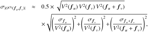$\begin{array}{ccc}{\mathit{\sigma }}_{\mathrm{\left|}{\mathit{O}}^{\mathrm{\left(}\mathrm{3}\mathrm{\right)}}\mathrm{\right(}{{f}}_{\mathit{u}}\mathit{,}{{f}}_{\mathit{v}}\mathrm{\left)}\mathrm{\right|}}& \mathrm{\approx }& \mathrm{0.5}\mathrm{\times }\sqrt{{\mathit{V}}^{\mathrm{2}}\mathrm{\left(}{{f}}_{\mathit{u}}\mathrm{\right)}\hspace{0.17em}{\mathit{V}}^{\mathrm{2}}\mathrm{\left(}{{f}}_{\mathit{v}}\mathrm{\right)}\hspace{0.17em}{\mathit{V}}^{\mathrm{2}}\mathrm{(}{{f}}_{\mathit{u}}\mathrm{+}{{f}}_{\mathit{v}}\mathrm{)}}\\ & & \end{array}$(A.2)where σ_fu, σ_fv and σ_{fu + fv} denote the errors of the measured squared visibilities. Another noise model for the bispectrum is described in Pauls et al. (2005).

Appendix B: Calculation of the spatial frequency density of data points

The presented algorithm reconstructs images from the measured four-dimensional bispectrum data O⁽³⁾(f_u,f_v). The measured squared visibilities are also elements of the bispectrum data because | O(f_u) | ² = O⁽³⁾(f_u,0) and O(0) = 1. Therefore, the density of bispectrum data points can be estimated by counting the number of data points inside a four-dimensional sphere centered at the spatial frequency coordinate of the considered bispectrum data point. The radius r₀ of the sphere is the smallest distance between two neighboring data points if all measured data points were equally distributed. Due to the symmetry of the bispectrum (Lohmann et al. 1983; Pflug et al. 1992), the total number of data points in the whole redundant four-dimensional bispectrum space is N = 12 N_b + 6 N_p, where N_b and N_p denote the numbers of closure phases and visibilities measured with an N_T-telescope array, respectively. For an N_T-telescope array and N_obs snap shots, N_p = N_obs × N_T (N_T − 1)/2 and N_b = N_obs × N_T (N_T − 1) (N_T − 2)/6. The volume of the whole

bispectrum plane is V_4d ≈ 9 | f_u,max | ⁴, where | f_u,max | is the length of the longest spatial frequency in the data measured. Therefore, from the empty volume around each equally distributed data point, or V_4d/ (12 N_b + 6 N_p), the smallest distance r₀ between two neighboring data points is given by ${\mathit{r}}_{\mathrm{0}}\mathrm{=}\mathrm{4}\sqrt{\frac{\mathrm{9}\hspace{0.17em}\mathrm{|}{{f}}_{\mathit{u,}\max }{\mathrm{|}}^{\mathrm{4}}}{\mathrm{12}\hspace{0.17em}{\mathit{N}}_{\mathrm{b}}\mathrm{+}\mathrm{6}\hspace{0.17em}{\mathit{N}}_{\mathrm{p}}}}\mathrm{=}\frac{\mathrm{\left|}{{f}}_{\mathit{u,}\max }\mathrm{\right|}}{\mathrm{4}\sqrt{\frac{\mathrm{4}}{\mathrm{3}}\hspace{0.17em}{\mathit{N}}_{\mathrm{b}}\mathrm{+}\frac{\mathrm{2}}{\mathrm{3}}\hspace{0.17em}{\mathit{N}}_{\mathrm{p}}}}\mathit{.}$(B.1)

Then the density of data points of the considered bispectrum element is inversely proportional to the number of data points within the four-dimensional sphere with radius r₀ centered at the position of that bispectrum element.

All Tables

All Figures

Fig. 1 Computer simulation of aperture-synthesis imaging with the IRBis image reconstruction method: a) uv coverage (see Table 1); b), c) intensity distribution of the two different disk-star computer targets (diameter 11.2 and 16.8 mas) (central star is clippped for display); d), e) intensity distribution of the targets convolved with the point spread function (PSF) of the simulated interferometer; f), g) examples of simulated interferograms (total number of interferograms is 250 per uv point) with 1219 and 573 photons per interferogram and simulated additive detector read-out noise (RON) of 10 electrons (the average value of the RON is subtracted); h) reconstructed images of the two targets for 10 e− RON and different photon numbers ⟨ N ⟩ per interferogram (from 1219 to 152). For each reconstruction, the labels give the corresponding average photon number ⟨ N ⟩ per interferogram, V2 S/N, CP error, χ2 function (Q1, Q2), regularization function (RG1, RG2, RG3, RG4, RG4b), χ2, residual ratio ρρ, and the restoration error ρ (see text).

In the text

Fig. 2 Dependence of the reconstructions on (a) the regularization functions H [ok(x)] used and (b) the χ2 function Q [ok(x)] applied in the cost function. This study shows reconstructions of the 16.8 mas disk-star target obtained in the experiment, as shown in Fig. 1 (for average S/N ~ 9 of the squared visibilities). Each row presents the reconstructions performed with one of the five regularization functions (RG1, RG2, RG3, RG4, and RG4b; see text and Eqs. (7)–(10)). The first two columns are reconstructions using the χ2 function Q1 [ok(x)] (see Eq. (4)) and the last two columns are reconstructions with the χ2 function Q2 [ok(x)] (see Eq. (5)). The columns labeled with “best qrec” are the reconstructions with the smallest value of qrec and those labeled with “best ρ” are the reconstructions with the smallest distance to the theoretical target. In each image, its restoration error ρ and its value of the reconstruction quality parameter qrec is presented.

In the text

Fig. 3 Same image reconstruction experiments as in Fig. 1 but with three different angular resolutions: (left column) resolution λ/D, or standard diffraction-limited resolution obtained by convolving the IRBis reconstruction with the diffraction-limited PSF of the interferometer, (middle column) resolution λ/2D (super-resolution), and (right column) IRBis reconstruction without convolving the original IRBis reconstruction with a PSF (i.e., some smoothing is only caused by regularization). The original synthetic target (diameter = 5.6 mas; see Table 2 for more details) is shown at the top with resolutions λ/D, λ/2D, and without any convolution (from left to right). For each reconstruction, the same information labels as in Fig. 1 are given. See text for more details.

In the text

Fig. 4 IRBis aperture-synthesis imaging of a synthetic T Tauri star-disk system submitted to the 2012 imaging beauty contest: (top panel) uv coverage, (middle panel, left) object, (middle panel, middle) object with resolution λ/D (=diffraction-limited resolution), (middle panel, right) object with resolution λ/2D (the original object was not known before the submission deadline of the beauty contest), (bottom panel, left) submitted IRBis reconstruction with resolution λ/D, and (bottom panel, right) submitted IRBis reconstruction with resolution λ/2D.

In the text

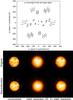	Fig. 5 Same as Fig. 4 but for the red supergiant target (see text).
In the text

References

- Baron, F., Cotton, W. D., Lawson, P. R., et al. 2012, in SPIE Conf. Ser., 8445 [Google Scholar]
- Buscher, D. F. 1994, in Very High Angular Resolution Imaging, eds. J. G. Robertson, & W. J. Tango, IAU Symp., 158, 91 [Google Scholar]
- Cornwell, T. J. 1983, A&A, 121, 281 [NASA ADS] [Google Scholar]
- Dai, Y.-H., Hager, W. W., Schittkowski, K., & Zhang, H. 2006, IMA J. Numer. Anal., 26, 604 [CrossRef] [Google Scholar]
- Hager, W. W., & Zhang, H. 2005, SIAM J. Optim., 16, 170 [Google Scholar]
- Hager, W. W., & Zhang, H. 2006, SIAM J. Optim., 17, 526 [CrossRef] [Google Scholar]
- Harries, T. J. 2011, MNRAS, 416, 1500 [NASA ADS] [CrossRef] [Google Scholar]
- Hofmann, K.-H., & Weigelt, G. 1993, A&A, 278, 328 [Google Scholar]
- Hofmann, K.-H., Driebe, T., Heininger, M., Schertl, D., & Weigelt, G. 2005, A&A, 444, 983 [NASA ADS] [CrossRef] [EDP Sciences] [Google Scholar]
- Ireland, M. J., Monnier, J. D., & Thureau, N. 2006, in SPIE Conf. Ser., 6268 [Google Scholar]
- Lawson, P. R., Cotton, W. D., Hummel, C. A., et al. 2004, in New Frontiers in Stellar Interferometry, ed. W. A. Traub, SPIE Conf. Ser., 5491, 886 [NASA ADS] [Google Scholar]
- Lawson, P. R., Cotton, W. D., Hummel, C. A., et al. 2006, in SPIE Conf. Ser., 6268 [Google Scholar]
- Lohmann, A. W., Weigelt, G., & Wirnitzer, B. 1983, Appl. Opt., 22, 4028 [NASA ADS] [CrossRef] [PubMed] [Google Scholar]
- Malbet, F., Cotton, W., Duvert, G., et al. 2010, in SPIE Conf. Ser., 7734, 83 [Google Scholar]
- Millan-Gabet, R., Monnier, J. D., Berger, J.-P., et al. 2006, ApJ, 645, L77 [NASA ADS] [CrossRef] [Google Scholar]
- Monnier, J. D., Barry, R. K., Traub, W. A., et al. 2006, ApJ, 647, L127 [NASA ADS] [CrossRef] [Google Scholar]
- Monnier, J. D., Anderson, M., Baron, F., et al. 2010, in SPIE Conf. Ser., 7734, 13 [Google Scholar]
- Narayan, R., & Nityananda, R. 1986, ARA&A, 24, 127 [NASA ADS] [CrossRef] [Google Scholar]
- Pauls, T. A., Young, J. S., Cotton, W. D., & Monnier, J. D. 2005, PASP, 117, 1255 [NASA ADS] [CrossRef] [Google Scholar]
- Pflug, L., Ioup, G., Ioup, J., & Field, R. 1992, J. Acoust. Soc. Am., 91, 975 [NASA ADS] [CrossRef] [Google Scholar]
- Rudin, L., Osher, S., & Fatemi, E. 1992, Phys. D, 60, 259 [NASA ADS] [CrossRef] [Google Scholar]
- Teboul, S., Blanc-Féraud, L., Aubert, G., & Barlaud, M. 1998, in Active contour models for segmentation and reconstruction on medical images, Asilomar Conf., USA [Google Scholar]
- ten Brummelaar, T. A., McAlister, H. A., Ridgway, S. T., et al. 2005, ApJ, 628, 453 [NASA ADS] [CrossRef] [Google Scholar]
- Thiebaut, E. 2002, in Astronomical Data Analysis II, eds. J.-L. Starck, & F. D. Murtagh, SPIE Conf. Ser., 4847, 174 [Google Scholar]
- Wahl, F. 1984, Digitale Bildverarbeitung (Heidelberg, New-York, Tokyo: Springer Verlag) [Google Scholar]