| Issue |
A&A
Volume 565, May 2014
|
|
|---|---|---|
| Article Number | A55 | |
| Number of page(s) | 11 | |
| Section | Stellar structure and evolution | |
| DOI | https://doi.org/10.1051/0004-6361/201322917 | |
| Published online | 08 May 2014 | |
CoRoT 105906206: a short-period and totally eclipsing binary with a δ Scuti type pulsator⋆,⋆⋆
1
INAF – Osservatorio Astronomico di Roma,
via Frascati 33, 00040
Monte Porzio Catone,
Italy
e-mail: This email address is being protected from spambots. You need JavaScript enabled to view it.
2
INAF – Osservatorio Astrofisico di Catania,
via S. Sofia 78, 95123
Catania,
Italy
3
Research and Scientific Support Department,
ESA/ESTEC, PO Box
299, 2200 AG
Noordwijk, The
Netherlands
4
Thüringer Landessternwarte Tautenburg,
Sternwarte 5, 07778
Tautenburg,
Germany
Received: 25 October 2013
Accepted: 19 March 2014
Abstract
Aims. Eclipsing binary systems with pulsating components allow determination of several physical parameters of the stars, such as mass and radius, that can be used to constrain the modeling of stellar interiors and evolution when combined with the pulsation properties. We present the results of the study of CoRoT 105906206, an eclipsing binary system with a pulsating component located in the CoRoT LRc02 field.
Methods. The analysis of the CoRoT light curve was complemented by high-resolution spectra from the Sandiford at McDonald Observatory and FEROS at ESO spectrographs, which revealed a double-lined spectroscopic binary. We used an iterative procedure to separate the pulsation-induced photometric variations from the eclipse signals. First, a Fourier analysis was used to identify the significant frequencies and amplitudes due to pulsations. Second, after removing the contribution of the pulsations from the light curve we applied the PIKAIA genetic-algorithm approach to derive the best parameters for describing the system orbital properties.
Results. The light curve cleaned for pulsations contains the partial eclipse of the primary and the total eclipse of the secondary. The system has an orbital period of about 3.694 days and is formed by a primary star with mass M1 = 2.25 ± 0.04 M⊙, radius R1 = 4.24±0.02 R⊙, and effective temperature Teff,1 = 6750 ± 150 K, and a secondary with M2 = 1.29 ± 0.03 M⊙, R2 = 1.34±0.01 R⊙, and Teff,2 = 6152 ± 162 K. The best solution for the parameters was obtained by taking into account the asymmetric modulation observed in the light curve, known as the O’Connell effect, presumably caused by Doppler beaming. The analysis of the Fourier spectrum revealed that the primary component has p-mode pulsations in the range 5–13 d-1, which are typical of δ Scuti type stars.
Key words: binaries: eclipsing / binaries: spectroscopic / stars: oscillations / stars: individual: CoRoT 105906206
Based on the photometry collected by the CoRoT satellite and on spectroscopy obtained with the Sandiford spectrograph attached at the 2.1-m telescope at McDonald Observatory (Texas, USA) and the FEROS spectrograph mounted on the ESO 2.2-m telescope at ESO (La Silla, Chile). The CoRoT space mission was developed and is operated by the French space agency CNES, with participation of ESA’s RSSD and Science Programs, Austria, Belgium, Brazil, Germany, and Spain.
Full Table 3 is only available at the CDS via anonymous ftp to cdsarc.u-strasbg.fr (130.79.128.5) or via http://cdsarc.u-strasbg.fr/viz-bin/qcat?J/A+A/565/A55
© ESO, 2014
1. Introduction
The study of eclipsing binary systems has gained a new perspective since the beginning of the CoRoT space mission (Baglin et al. 2006). The superb photometry achievable from space, combined with ground-based spectroscopy, allows a precise and independent determination of mass and radius of the components, among other parameters. In particular, by studying pulsating stars in eclipsing binaries, such as the Classical γ Dor and δ Sct type variables, one takes advantage of this parameter determination for the asteroseismic modeling of stellar structure and evolution. The CoRoT observations unveiled several targets suitable for this kind of research.
The δ Sct type variables are stars located in the classical instability strip on the H-R diagram with effective temperatures in the range 6300 < Teff < 9000 K, luminosities 0.6 < log (L/L⊙) < 2.0, and masses between 1.5 and 2.5 M⊙. Their evolutionary stages range from pre-main sequence to just evolved off the main sequence (about 2 mag above the ZAMS). They exhibit radial and/or nonradial pulsations, with low-order gravity (g) and/or pressure (p) modes with pulsation periods ranging from ∼15 min to ∼8 h (see, e.g., Rodríguez & Breger 2001; Buzasi et al. 2005; Uytterhoeven et al. 2011).
As a result, δ Sct type stars are an interesting class of objects since they lie in the transition region between stars having a convective (M < 2 M⊙) or a radiative (M > 2 M⊙) envelope. Their masses are in a range where stars are developing a convective zone, so they are useful for better understanding the mechanisms responsible for driving the pulsations. In this work we describe the analysis of CoRoT 105906206, an eclipsing binary system showing properties typical of δ Sct type variables.
Sections 2 and 3 present the details of the photometric and the spectroscopic observations, respectively. Section 4 describes how we derive the parameters of the system through the analysis of the light and radial-velocity curves, and Sect. 5 provides additional physical properties. The resulting pulsation frequencies are discussed in Sect. 6, and our final remarks and conclusions are in Sect. 7.
2. CoRoT photometry
CoRoT 105906206 was observed during the second “Long Run” in the direction of the Galactic center (LRc02), which lasted about 161 days. According to the information in the ExoDat database (Deleuil et al. 2009), this relatively bright target (V = 11.784 ± 0.044 mag) has a low level of contamination (L0 = 0.0077, where L0 is the ratio between contaminant and total fluxes) and thus was not removed from the observed flux. Our analysis used a white light curve, which is the sum of the three chromatic light curves from the CoRoT three-color photometry (Auvergne et al. 2009). These colors (red, green, and blue channels) do not represent any standard photometric system. They were implemented to help with the identification of false alarms that can mimic the transit of a planet in front of the main target.
The original time series, containing about 388 000 points, was detrended to remove long-term variations and was cleaned from outliers using a sigma-clipping algorithm. Points flagged according to the description of Gruberbauer (2008) were also excluded. Only a few measurements (corresponding to about 0.5 days) were made in the long-integration mode (512 s) and they were not used in our analysis. The resulting light curve contains about 341 000 points collected in the short-integration mode (32 s), from HJD = 2 454 573 to 2 454 717 days. A portion of the processed light curve is shown in Fig. 1.
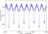 |
Fig. 1 Portion of the CoRoT 105906206 white light curve normalized to the mean value. The full data extends over 144 days. |
3. High-resolution spectroscopy
We collected high-resolution spectra of CoRoT 105906206 using two instruments: the Sandiford Echelle Spectrograph (McCarthy et al. 1993) attached to the Cassegrain focus of the 2.1-m telescope of McDonald Observatory (Texas, USA), and the fiber-fed FEROS Echelle Spectrograph (Kaufer et al. 1999) mounted on the MPG/ESO 2.2-m telescope at La Silla Observatory (Chile).
Six Sandiford spectra were taken over six consecutive nights in May 2011 under fairly good sky conditions, with seeing typically varying between 1.0 and 2.0′′. We set the grating angle to cover the wavelength range 5000–6000 Å and used the 1.0′′ wide slit, which yields a resolution of R ∼ 47 000. We adopted an exposure time of 1200–1800 sec and traced the radial velocity drift of the instrument by acquiring long-exposed (Texp = 30 s) ThAr spectra right before and after each epoch of observation.
Nineteen additional spectra were acquired in June and July 2011 with FEROS, which provides a resolution of R ∼ 48 000 and covers the wavelength range ∼3500–9200 Å. The sky conditions were photometric throughout the whole observation run, with seeing between 0.6 and 1.0′′. Exposure times ranged between 1200 and 1800 s.
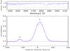 |
Fig. 2 Example of cross-correlation used to derive the radial velocities of the CoRoT 105906206 components. Top panel: a portion of FEROS spectra showing the regions used (delimited by horizontal bars). Bottom panel: cross-correlation peaks of the primary (1) and secondary (2) stars (dots) fitted by a double-Gaussian function (solid line). |
The spectra were reduced using IRAF1 standard routines and the FEROS automatic pipeline for order identification and extraction, background subtraction, flat-field correction and wavelength calibration. The radial velocities of the two components, together with their uncertainties, were derived with the fxcor task of IRAF by cross-correlating each spectrum with a reference template. The standard stars HD 168009 (Udry et al. 1999) and HD 102870 (Nidever et al. 2002), both observed with the same instrumental set-up, were used as template for Sandiford and FEROS spectra, respectively. Figure 2 shows the cross-correlation function (CCF) peaks fitted by a double Gaussian curve. The uncertainty in each radial-velocity measurement and the fit of one or a double Gaussian depend on the separation of the peaks.
In the beginning of our study, we made a visual comparison of our spectra with the Digital Spectral Classification Atlas of R. O. Gray2. It suggested a spectral type F3 for the primary star, corresponding to an effective temperature of about 6800 K. This is the value we used in this work, though it was later improved by the spectroscopic analysis of the primary decomposed spectrum, obtained through the disentangling method (see Sect. 3.1). At any rate, these determinations are in very good agreement. Concerning the secondary companion, it only makes a small contribution to the total flux, as can be seen in Fig. 2.
The derived radial velocities and the estimated uncertainties of the two stars of CoRoT 105906206 are listed in Table 1 and plotted in Fig. 3, together with the best-fit models computed with the PHOEBE code (PHysics Of Eclipsing BinariEs, Prsa & Zwitter 2005) for both primary and secondary components. Besides Keplerian motion, the models also consider the Rossiter-McLaughlin (R-M) effect.
Radial velocities of CoRoT 105906206.
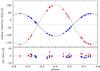 |
Fig. 3 Phase-folded radial velocities of CoRoT 105906206 (top panel) and residuals of the best-fit models (bottom panel). Filled circles and triangles are FEROS and Sandiford measurements, respectively. Uncertainties are shown in light gray. The best Keplerian plus R-M models, obtained with PHOEBE, are shown as continuous and dashed lines for primary and secondary components, respectively. |
3.1. Spectral decomposition
The VO-version3 of the KOREL program (Hadrava 2004, 2009) was used to decompose the FEROS spectra into the individual stellar components. The method of spectral disentangling was first introduced by Simon & Sturm (1994) and later on reformulated by Hadrava (2004) in the Fourier space.
The quality of the spectral disentangling performed with KOREL strongly depends on the quality of the derived line shifts of the components (radial velocities). To determine these shifts as precisely as possible, we excluded the broad Balmer lines from this step of the analysis. From visual inspection, we could only find one line of the secondary component in the spectra, Mg ii at 5183 Å. A first KOREL solution was computed on a small interval around this wavelength, and then the region was extended to the range 4915 to 5500 Å, also allowing for variable line strengths in the program. Any further extension in wavelength did not improve the accuracy of the results. Because of the low frequency problem typical of Fourier transform-based disentangling programs like KOREL (see, e.g., Hensberge et al. 2008), slight undulations occurred in the computed continua of the decomposed spectra. Therefore, we applied KOREL to overlapping 20 nm wide bins, where we fixed the orbital parameters and time variable line strengths to the values obtained before. Only in the case of broad Balmer lines did we choose wider bins. Each piece of decomposed spectrum, which in total covers a wavelength range from 4410 to 6860 Å, was corrected for slight continuum undulations using spline fits. Finally, all bins were merged using weighting ramps for the overlapping parts.
KOREL delivers the decomposed spectra of the components normalized to the common continuum of both stars. A renormalization to the individual continua of the components can only be done by assuming a value for their flux ratio. Since this value is very low, the line depths of the secondary are very sensitive to the flux ratio. This, in addition to the very low signal-to-noise ratio (S/N) of the decomposed secondary spectrum, prevented us from its analysis. In the case of the primary, small deviations from the true flux ratio only cause a second-order effect.
For the spectral analysis of the primary component, we assumed a flux ratio of 0.07 that was estimated from the light-curve solution (the ratio between the bolometric luminosities listed in Table 2). We used the ATLAS9 plane-parallel and LTE model atmospheres (Kurucz 1993) and calculated synthetic spectra using SPECTRUM, a stellar spectral synthesis code (Gray & Corbally 1994). We convolved the synthetic spectra with a Gaussian profile having a FWHM = 0.11 Å, to account for the spectrograph resolution, and adopted a surface gravity of log g = 3.53 ± 0.01 dex, as derived from the modeling of the eclipsing binary.
Parameters of CoRoT 105906206 from PHOEBE fits of light and radial-velocity curves.
We derived the effective temperature by fitting the wings of the Hα and Hβ Balmer lines, and the iron abundance ([Fe/H]) together with the microturbulence velocity (υmicro) by applying the method described in Blackwell & Shallis (1979) on isolated Fe i and Fe ii lines. The results are Teff,1 = 6750 ± 150 K, [Fe/H] = 0.0 ± 0.1 dex, and υmicro,1 = 2.5 ± 0.8 km s-1. We also measured the projected rotational velocity υsini of the stars i) by fitting the CCF profile of individual FEROS spectra using the rotation profile described in Gray (1976), which was convolved with the instrumental profile; and ii) by fitting the profile of several clean and unblended metal lines. We derived υ1sini = 47.8 ± 0.5 km s-1 and υ2sini = 19 ± 3 km s-1 from the CCF peaks for both primary and secondary stars, and υ1sini = 46 ± 2 km s-1 from the metal lines of the decomposed spectrum of the primary. As a matter of fact, the value of υsini that we derive here is a mix of velocity fields including stellar rotation, macroturbulence, and pulsations. However, given the high rotation rate of these stars, the macroturbulence and the pulsation broadening are second-order effects.
We also derived the abundance of chemical elements other than iron using the decomposed spectrum of the primary star. However, the continuum undulations produced by the disentangling procedure, though we tried to correct them, may still affect the abundance determination, specially for heavy elements, which have a small number of spectral lines available. Nevertheless, for elements lighter than Fe, the abundances mostly follow the solar values (Asplund et al. 2005).
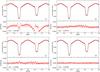 |
Fig. 4 Phase-folded light curve (the top of each panel) and residuals of the best-fit (the bottom of each panel) for models a) with gravity darkening and surface albedo coefficients fixed at β = 0.32 and A = 0.60, b) with A1, A2, and β1 set as free parameters but without accounting for the Doppler beaming, c) with A1, A2, β1, and B set as free parameters but still keeping the oscillations (see Sect. 4.1) and d) removing the oscillations. |
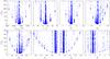 |
Fig. 5 Reduced chi-square between model and data as a function of the eight free parameters of the light curve model computed using the PIKAIA genetic algorithm during the search for the best solution. From left to right, and from top to bottom: secondary effective temperature, orbital inclination angle, surface potentials, primary gravity darkening, surface albedos, and beaming factor. |
4. Light and radial-velocity curve analysis
The binary model for both light and radial-velocity curve of CoRoT 105906206 were computed with PHOEBE, a tool for eclipsing binary modeling based on the Wilson-Devinney code (Wilson & Devinney 1971). The search for the best model was performed with the PIKAIA subroutine (Charbonneau 2002), a genetic-algorithm based approach. PIKAIA maximizes a user-supplied function (=1/χ2) by minimizing the chi-square χ2 between model and data. It starts with a so-called “population”, formed by a given number of “individuals” which, in turn, are formed by sets of parameters randomly selected within a given range of the parameter space. These sets of parameters are encoded as strings to form a “chromosome-like” structure and represent the first trial solutions. The initial solutions (or “parents”) then evolve through subsequent “generations” of possible solutions (the “offsprings”), following rules similar to typical processes of the biological evolution (breeding, crossover, mutation). In equivalence to the natural selection, only solutions that provide low values of χ2 are passed to the next generations, and the final solution is achieved after some condition is satisfied.
Our supplied function evaluates the χ2 between the observed light curve and the models computed for a set of free parameters that characterize the orbital and physical properties of a binary system. Following the same procedure as described in Maceroni et al. (2014), we implemented this function in a FORTRAN-based routine, FITBINARY, which makes use of Wilson-Devinney routines to compute the binary models. In our FITBINARY code we adopt the PIKAIA 1.2 new version, an improvement of PIKAIA 1.0 that includes additional genetic operators and algorithm strategies. In particular, the new version allows several mutation modes, such as a fixed or an adjustable mutation rate based either on fitness (the value of 1/χ2 comparing best and median individuals) or on distance (the metric distance between best and median population clustering). We normally adopted an initial population with 100 individuals evolving through 200 generations, a mutation mode of one-point+creep and adjustable rate based on fitness, and a full generation replacement with elitism. The other control parameters were normally kept fixed at their default values (see the related documentation in the PIKAIA Homepage4).
In the prewhitening process, described in detail in Sect. 4.2, (i) we first remove an initial binary model from the processed light curve (the one resulting from the cleaning steps of Sect. 2); then (ii) we identify the significant frequencies in the amplitude spectrum of the time series with oscillations only; (iii) we subtract the frequencies from the processed light curve; and finally (iv) we search for an improved solution for the binary model applied to the light curve with the eclipses alone. These steps are repeated until there is no improvement in the last solution. However, by using this procedure to treat the whole data set (of about 144 days), we did not find any satisfying solution, and the remaining residuals still had clearly visible oscillations. This does not happen if we apply the same procedure to a segment of light curve, since the residuals in this case are at least 2.5 times smaller. We therefore divided the light curve into 8 segments of about 20 days each and applied the procedure of prewhitening to each one separately. In the following sections we present the results obtained using the first segment of the light curve, and at the end of the paper we comment on the comparison with what we obtain using the other segments.
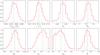 |
Fig. 6 Distributions of the parameters resulted from our Markov chain Monte Carlo (MCMC) simulations. The histograms are normalized to unit and contain 40 000 accepted solutions each. The median of each distribution and the limits enclosing 68% of the results (with equal probability in both sides) are indicated by the dashed lines, and represent the values listed in Table 2. The solid lines indicate the solution that minimizes χ2. |
4.1. Preliminary solutions
First, using PHOEBE and the radial-velocity data alone, we searched for a good solution
to the orbital model by changing the orbital period P, the semi-major axis
a, the
secondary-to-primary mass ratio q, and the barycentric velocity υγ. Then, keeping fixed
the derived values (except P), we improved the orbital period and, with PIKAIA,
we searched for a solution that best fits the light curve data by changing the secondary
effective temperature Teff,2, the orbital
inclination angle i, and the surface potentials Ω1 and Ω2. The eccentricity
e and the
longitude of periastron ω0 were kept fixed at zero, and the
primary effective temperature Teff,1 was set to 6800
K (according to our estimate performed in Sect. 3).
The ratio between orbital and rotation periods was fixed to f = 1.0 for both
companions. Later on, with our estimate of the projected rotation velocity from the CCF
peaks (see Sect. 3.1), we derived Prot,1 = 4.44
± 0.07 days and
Prot,2 =
 days (assuming coplanarity between
equatorial and orbital planes, as discussed in Sect. 7), which yielded f1 = 0.83 ± 0.01 and
days (assuming coplanarity between
equatorial and orbital planes, as discussed in Sect. 7), which yielded f1 = 0.83 ± 0.01 and
 . However, these new values did not
significantly affect the results already found for the parameters.
. However, these new values did not
significantly affect the results already found for the parameters.
Concerning the limb darkening, we adopted a square-root law with two coefficients, xLD and yLD, for each component and these coefficients also depend on the passband intensities. For a given set of photospheric parameters, PHOEBE interpolates the limb darkening coefficient tables computed for CoRoT passbands (see Maceroni et al. 2009). For both stars, the bolometric luminosity L, mass M, radius R, and surface gravity log g were computed rather than adjusted, where R represents the radius of a sphere with the same volume as the modeled star.
This first preliminary solution model for a detached binary, which is shown in Fig. 4a, is based on the cleaned light curve described in
Sect. 2, including the pulsations and other kinds of
periodic patterns. The curve was binned using an average of 1000 points in both time and
flux in the phase-folded space. The gravity darkening and surface albedo coefficients were
kept fixed at β = 0.32 and A = 0.60 for purely
convective envelopes (Lucy 1967), by adopting
 .
.
Claret (1999) computed the gravity darkening as a function of mass and degree of evolution of the star, which resulted in a smooth transition between convective and radiative energy transport mechanisms. Therefore, in a second step, the gravity darkening (except β2) and surface albedos were set as free parameters as an attempt to improve the fit (see Fig. 4b). Since the primary luminosity dominates the observed flux, the models are independent of the secondary gravity darkening, and therefore β2 was kept fixed (see Table 2).
As can be seen in Fig. 4b, and more clearly in the
residuals plot, there is a modulation pattern, commonly referred to as the O’Connell
effect (O’Connell 1951), in which the flux maximum
after the deeper eclipse is greater than the maximum after the shallower eclipse (see also
Milone 1968; Davidge & Milone 1984). Some attempted explanations for this asymmetric
modulation are the presence of spots on the surface of a chromosphericaly active star,
circumstellar clouds of gas and dust, or a hot spot created by mass transfer. Given the
physical configuration of this system, however, both stars are nearly spherical (see Sect.
5), so the scenario of mass transfer can be safely
excluded from the list of possible causes of the O’Connell effect. Another possible
explanation is instead the so-called Doppler beaming, in which the orbital movement of the
star modifies its apparent luminosity by beaming the emission of photons in the direction
of the observer. The relation (adapted from Loeb &
Gaudi 2003) between emitted (F0,λ) and observed
(Fλ) flux is
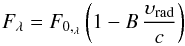 (1)where B is the beaming factor
(see also Zucker et al. 2007; Bloemen et al. 2011), which depends on the wavelength of the
observations and on the physical characteristics of the star. In a binary system, since
the stars move in opposite directions with respect to the observer, the net beaming effect
represents the difference in flux between the components. Therefore, there is no
modulation caused by the Doppler beaming if the binary components have the same mass and
the same spectral type. To account for and remove this modulation pattern from the
observed light curve, we searched for a binary model in which the emitted flux is
transformed according to Eq. (1), and the
beaming factor is set as a free parameter (see Fig. 4c and Table 2).
(1)where B is the beaming factor
(see also Zucker et al. 2007; Bloemen et al. 2011), which depends on the wavelength of the
observations and on the physical characteristics of the star. In a binary system, since
the stars move in opposite directions with respect to the observer, the net beaming effect
represents the difference in flux between the components. Therefore, there is no
modulation caused by the Doppler beaming if the binary components have the same mass and
the same spectral type. To account for and remove this modulation pattern from the
observed light curve, we searched for a binary model in which the emitted flux is
transformed according to Eq. (1), and the
beaming factor is set as a free parameter (see Fig. 4c and Table 2).
4.2. Final solution, uniqueness, and uncertainties
The plots in Figs. 4a–c are based on the light curve with the oscillations still present. These include those stemming from stellar pulsations and other sources, such as the orbital period of the CoRoT satellite (103 min) and its harmonics. We use an iterative procedure for the prewhitening. First we find the best fit to the light curve setting the secondary effective temperature, orbital inclination angle, surface potentials, the albedo coefficients of both components, the primary gravity darkening, and the beaming factor as free parameters (Fig. 4c). After that we subtract this model from the observed data so that only oscillations remain.
We then used Period04 (Lenz & Breger 2005), a program developed for the analysis of time series, to compute the Fourier spectrum and to search for the frequency, amplitude, and phase of each sinusoidal component of the signal. To establish the number of components that give a significant contribution to the signal, we applied the commonly used criterion of S/N > 4, i.e., only frequencies having an amplitude four times the local noise are considered. It is worth noting that, in order to avoid spurious frequencies in the amplitude spectrum, small gaps in the time series were filled in with artificial points that follow a polynomial function fitted to adjacent regions of each gap. A noise consistent with the dispersion of the adjacent regions was applied to each point. More details on the pulsation frequencies are described in Sect. 6.
Finally, the significant frequencies (according to the criterion mentioned above) were subtracted from the cleaned light curve leaving only the eclipses and the modulation of the binary. Again, using PIKAIA and PHOEBE, we improved the preliminary values of Teff,2, i, Ω1, Ω2, A1, A2, β1, and B. The procedure was repeated until the χ2 value between model and data did not decrease significantly.
We also tried to account for the individual flux contribution of each star to the observed pulsations in and out of eclipse. However, since the primary star is the pulsating component (we get to this conclusion in Sect. 6) and dominates the observed flux, the influence of the secondary component on the observed pulsations is negligible, because smaller than the noise. We were thus unable to see any difference in the pulsations amplitude in and out of eclipse, and the pulsation frequencies found were equally subtracted from the entire light curve.
The minimization algorithms employed by PHOEBE are the commonly used Levenberg-Marquandt
and Nelder & Mead’s downhill simplex, both of which are nonlinear optimization methods
affected by the problem of remaining stuck at local minima. In the PIKAIA genetic
algorithm, mutation and crossover allow the population to move away from local solutions.
Figure 5 plots the reduced chi-square
 (where ν = N − n
− 1 is the number of degrees of freedom for N observation points and
n fitted
parameters) as a function of the free parameters of the light curve model, for a wide
range of the parameter space. PIKAIA tries several local solutions (pattern of points
vertically assembled) and progressively moves towards the global minimum. In any case, we
preferred to carry out more than one iteration, and also around a narrower range of the
parameter space, to better constrain the solutions that provide the minimum
χ2.
(where ν = N − n
− 1 is the number of degrees of freedom for N observation points and
n fitted
parameters) as a function of the free parameters of the light curve model, for a wide
range of the parameter space. PIKAIA tries several local solutions (pattern of points
vertically assembled) and progressively moves towards the global minimum. In any case, we
preferred to carry out more than one iteration, and also around a narrower range of the
parameter space, to better constrain the solutions that provide the minimum
χ2.
To estimate the uncertainties in the parameters we performed Markov chain Monte Carlo (MCMC) simulations using the Metropolis algorithm (see, e.g., Gelman et al. 2003; Ford 2005). This method is based on a Bayesian inference in the sense that the posterior (or desired) probability distribution p(x|d) of a set of parameters x given the observed data d is proportional to the product of a prior knowledge of the probability distribution of the parameters p(x) and a factor exp[−χ2(x)/2], which depends on the χ2 goodness of the fit adopting the model x. For the prior probability function, we adopted a Gaussian distribution, centered on an initial set of x and having initial arbitrary variances. The idea is to construct a parameter space that approximates the desired probability distribution. To do so, we generated a chain (or sequence) formed by sets of random parameters that are sampled according to the prior probability distributions. If a set of parameters x′ yields a χ2 that is smaller than the previous one, then the new solution is accepted. Otherwise, this new solution is accepted with probability exp[−[χ2(x′) − χ2(x)/2]].
The acceptance rate can be adjusted by multiplying the initial variances by a scaling factor, in order to optimize the number of accepted solutions. We redefine this scaling factor every 100 steps of the simulations to achieve a ratio of about 0.25 between the accepted and the total number of generated solutions, which is an optimal value for a multidimensional space (see Gelman et al. 2003). During a first phase of tests, which is called the burn-in phase, the variances of the prior distributions are constantly updated (they are computed from the posterior distributions themselves). The uncertainty on the data is also adjusted to ensure that the value of minimum χ2 is equal to the number of degrees of freedom. The burn-in solution is then discarded and a new simulation begins. After reaching a certain number of accepted solutions, the posterior probability distributions become stable and the chain converges toward the desired distribution.
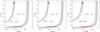 |
Fig. 7 Evolution of the radius of the system components in the mass range M1,2 ± 2σ(M1,2) (shaded regions, from Table 2) for three values of chemical composition. The darker regions represent the intersection with R1,2 ± 2σ(R1,2) (horizontal lines, also from Table 2). The vertical lines indicate the limits in age according to the constraint of coevality of the two stars. |
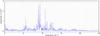 |
Fig. 8 Amplitude spectrum of CoRoT 105906206 after subtracting the final binary model. The vertical dashed lines represent multiples of the orbital frequency (Forb = 0.270667 d-1). |
Figure 6 plots the distributions of the eight free parameters that we used to model the light curve of CoRoT 105906206. We discarded the first 15% of the accepted solutions, and the histograms contains 40 000 points each. The parameters of the best-fit solution and their uncertainties are listed in Table 2. They represent the median values and the 68% confidence limits shown in the figure, and are in very good agreement with the best solution found with PIKAIA. It is worth noting that, since Teff,2 is correlated with Teff,1 (because of the degeneracy between the effective temperatures and the passband luminosities), the uncertainty estimated for the secondary temperature also accounts for the one estimated for the primary star. The final light curve model is shown in Fig. 4d.
First 50 pulsation frequencies, amplitudes, and phases derived for CoRoT 105906206 after subtracting the final binary model.
5. Physical properties of CoRoT 105906206
Besides the parameters that come directly from the fits of the light and radial-velocity curves, the masses (M1 and M2), radii (R1 and R2), and surface gravities (log g1 and log g1) of the two stars are also calculated. Using the values of radius and effective temperature, we can calculate the luminosities (L2 and L1). All these parameters, together with the limb darkening coefficients (xLD,1, xLD,2, yLD,1, yLD,2), are listed in Table 2. The resulting model is for a detached binary, whose components are both nearly spherical. For the primary, the radius in the direction toward the secondary is about 4% larger than the radius in the direction of the stellar pole. For the secondary this value is only about 0.3%. This shows that even the primary star is far from reaching the Roche lobe.
To estimate the age of the system, we used the Yonsei-Yale (Y2) evolutionary tracks (Yi et al. 2003), interpolated in mass and chemical composition and drawn on the radius vs. age diagram. This kind of diagram allows us to see the evolution of the stellar radius with time. It is preferred over using the placing of the stars in the H-R diagram because, in eclipsing binary systems, we have a precise determination of mass and radius of the components. We checked the effective temperatures of each star that come from the evolutionary models, and they are consistent with those derived from our spectral and light curve analyses.
Figure 7 shows the radius vs. age diagrams for three
values of metallicity in the range [Fe/H] ± 2
σ
([Fe/H]), from Sect. 3.1, plotted for
masses and radii in the range M1,2 ±
2σ(M1,2)
and R1,2 ±
2σ(R1,2),
both from Table 2. Applying the constraint of
coevality of the two stars, we found the age of this binary system to be
 Myr. These are 1σ uncertainties, though, for
clarity in the figure, the diagrams were constructed within two standard deviations in
metallicity, mass, and radius. The sharp vertical drops correspond to the second
gravitational contraction at the end of main-sequence stars. To compute the evolutionary
tracks, an overshoot parameter αOV = 0.2 HP (units of the pressure
scale height) is adopted when a convective core develops (see Yi et al. 2003, and references therein).
Myr. These are 1σ uncertainties, though, for
clarity in the figure, the diagrams were constructed within two standard deviations in
metallicity, mass, and radius. The sharp vertical drops correspond to the second
gravitational contraction at the end of main-sequence stars. To compute the evolutionary
tracks, an overshoot parameter αOV = 0.2 HP (units of the pressure
scale height) is adopted when a convective core develops (see Yi et al. 2003, and references therein).
6. Pulsation properties
Figure 8 shows the amplitude spectrum of CoRoT 105906206, computed using Period04 after subtracting the final binary model from the light curve. We searched for significant peaks up to the Nyquist frequency, but none was found beyond 25 d-1. A total of 220 frequencies with S/N > 4 was identified, and Table 3 lists the first 50, together with the amplitudes and phases, and the respective formal errors computed according to Montgomery & O’Donoghue (1999). We also searched for possible frequency combinations, including the orbital frequency (Forb = 0.270667 d-1). The most evident are listed in the last column of this table. We identified a few combinations that involve the orbital frequency and the most dominant peaks F1, F2, F3, and F5, which seem to be genuine p-mode frequencies. A few overtones of the orbital period are still present in Fig. 8, and are also indicated in Table 3. They are probably residuals of the prewhitening process, but have small amplitudes.
The typical properties of δ Sct type variables in terms of effective temperature,
luminosity, mass, evolutionary stage, and pulsation frequency range are all present in the
primary component of CoRoT 105906206, as one can see in Table 2 and in the list of dominant frequencies in Table 3. As an rough estimate of the frequency range of the pulsations, we
applied the relation between the frequency of a given radial mode Fpuls, the stellar
mean density  , and the pulsation constant Q:
 (2)From the fundamental to the fifth radial mode,
we have 0.033 ≲ Q ≲
0.013 (Stellingwerf 1979), which
yields 5.2 ≲ Fpuls ≲
13.2 d-1 if we use the values of mass and radius of the
primary star, a range that contains the most significant frequencies seen in Fig. 8. The same computation for the secondary star yields
frequencies in the range 22 ≲
Fpuls ≲ 56 d-1, which are not
observed in the amplitude spectrum. This confirms that the identified pulsation modes belong
the primary component.
(2)From the fundamental to the fifth radial mode,
we have 0.033 ≲ Q ≲
0.013 (Stellingwerf 1979), which
yields 5.2 ≲ Fpuls ≲
13.2 d-1 if we use the values of mass and radius of the
primary star, a range that contains the most significant frequencies seen in Fig. 8. The same computation for the secondary star yields
frequencies in the range 22 ≲
Fpuls ≲ 56 d-1, which are not
observed in the amplitude spectrum. This confirms that the identified pulsation modes belong
the primary component.
From the theoretical point of view, a nonadiabatic analysis of an equilibrium model with the physical properties of the primary component, performed with the nonadiabatic oscillation code MAD (Dupret et al. 2005), provides excited modes with frequencies in the typical domain of δ Sct type stars, namely: from 5.2 to 17.0 d-1 in the fundamental mode (ℓ = 0), from 4.0 to 16.6 d-1 in the ℓ = 1 mode, and from 4.2 to 16.7 d-1 in the ℓ = 2 mode, which are in line with the observed range of pulsation frequencies.
7. Final remarks and conclusions
The study of CoRoT 105906206 unveiled an eclipsing binary system in which the primary component pulsates in the range of frequencies typical δ Sct type variables, a result that agrees with the derived values of effective temperature, luminosity, mass, and stage of evolution. Moreover, from the theoretical point of view, a nonadiabatic analysis of a model matching the physical properties of the primary star gives excited frequencies of the most relevant modes (ℓ = 0, 1, and 2) in the same frequency range of the observed pulsations.
By allowing the surface albedos and gravity darkening to vary as free parameters, we improved the solution for the binary model in comparison with the model found by keeping them fixed. In particular, our estimate of β1 agrees with the calculations of Claret (1999) for the gravity darkening as a function of the effective temperature for a 2 M⊙ star.
An interesting characteristic of this system is the presence of the O’Connell effect, an asymmetric photometric modulation pattern that we interpreted as due to the Doppler beaming of the emitted flux. We quantified this effect by means of the beaming factor B, whose value depends on the passband of the photometric observations and on the physical properties of the stars. Using equations from Mazeh & Faigler (2010), our Eq. (1), and some of the parameters in Table 2, we obtain B = 2.00 ± 0.05, which is in fair agreement with the beaming factor derived from the light curve model (see Table 2). The αbeam factor used in those equations was set to unity. This factor accounts for the effect of the stellar light being shifted out or into the observed passband. According to Faigler & Mazeh (2011), the value of αbeam may range from 0.8 to 1.2 for F, G, and K stars observed with the CoRoT passband. The same beaming factor listed in Table 2 is obtained setting αbeam = 0.8.
That the primary star rotates with a subsynchronous velocity may generate some doubt about our determination of the rotation period, and motivated us to provide some tentative explanations. A spin-orbit misalignment, for example, would lead to overestimating Prot,1. However, using Eq. (22) of Hut (1981) applied to the parameters derived for this system and assuming that the primary component rotates as a rigid body, we can estimate the ratio of orbital to rotational angular momentum to be α ∼ 30. In Fig. 4 of that paper, for this value of α, the time scale for circularization is much longer than the time for alignment. Therefore, if e = 0, which is the case of our system, no misalignment is expected. Another explanation could be the loss of angular momentum due to mass transfer. However, the system components are both nearly spherical and far from filling the Roche lobe. The most plausible explanation seems to be the radius expansion of the primary component related to its stage of evolution. This star is passing through a region on the H-R diagram of roughly constant luminosity, decrease in effective temperature, and increase in radius. According to the grid of stellar models with rotation of Ekström et al. (2012), a star of about 2 M⊙ that has just evolved off the main sequence will pass through a phase of decreasing equatorial velocity before reaching the base of the giant branch (see their Fig. 9). Though these models were computed for single stars, and not specifically for a star with the same parameters as the primary component of our system, they give us an indication that a decrease in the rotation rate is possibly taking place.
The division of the light curve into 8 segments of about 20 days each was needed to identify the bona fide pulsation frequencies. A shift in the frequency phases with time seems to disturb the identification of frequencies in the whole time series. We performed several tests for phase shifts in the pulsation frequencies and for identifying any periodical variation. However, even if phase shifts are indeed present, no clear periodical variation was found. We are not able to explain the origin of this variation, though we think that it is likely intrinsic to the star. The data reduction process and an instrument-related effect could be the cause, but we have applied the same method to several other light curves of both CoRoT and Kepler systems, and we have not seen the same behavior before.
We derived our results based on the first of the eight segments. We tested the others by proceeding with the prewhitening steps, which led to new solutions for the binary models, and to identifying pulsation frequencies in each segment. A comparison of the fitted parameters shows very good agreement and low dispersion among the segments. The mean values are ⟨Teff,2⟩ = 6162 ± 13 K, ⟨ i ⟩ = 81.66 ± 0.15◦, ⟨ Ω1 ⟩ = 4.27 ± 0.02, ⟨ Ω2 ⟩ = 7.89 ± 0.05, ⟨ β1 ⟩ = 0.52 ± 0.02, ⟨ A1 ⟩ = 0.77 ± 0.11, ⟨ A2 ⟩ = 0.06 ± 0.08, and ⟨ B ⟩ = 1.48 ± 0.04. The dispersions are of the order of or smaller than the estimated uncertainties, and the values agree with those in Table 2. Regarding the analysis of the pulsation frequencies, the peaks with higher amplitudes in Fig. 8 (> 1 × 10⁻³) were normally identified in all the eight segments of the light curve, in particular the four genuine p-modes (F1, F2, F3, and F5) listed in Table 3. Small shifts in amplitude, probably related to the phase shifts, were also observed among the segments.
We believe it would be useful to have more spectra collected during the eclipses in order to allow modeling the Rossiter-McLaughlin effect. This would confirm whether the spin-orbit axes are indeed aligned, as we suspect, and reinforce the possibility of radius expansion of the primary star owing to its stage of evolution. The gathering of more spectra, with higher S/N, would also improve the precision achieved in the spectroscopic analysis, yielding an accurate abundance determination of elements other than iron. We also believe that the behavior of the amplitude and phase variations is still not well understood. The development of more robust programs and methods for analyzing of time series is required to properly deal with this kind of data, in which a large number of observation points and pulsation frequencies are present.
Image Reduction and Analysis Facility, distributed by the National Optical Astronomy Observatories (NOAO), USA.
Acknowledgments
We thank Josefina Montalbán and Marc-Antoine Dupret for the nonadiabatic calculation of the excited pulsation frequencies. We are also very grateful for the referee report to this work, which contributed a lot to improving our manuscript. This research made use of the ExoDat Database, operated at LAM-OAMP, Marseille, France, on behalf of the CoRoT/Exoplanet program, and was accomplished with the help of the VO-KOREL cloud service, developed at the Astronomical Institute of the Academy of Sciences of the Czech Republic in the framework of the Czech Virtual Observatory (CZVO) by P. Skoda and L. Mrkva using the Fourier disentangling code KOREL by P. Hadrava. We acknowledge the generous financial support by the Istituto Nazionale di Astrofisica (INAF) under Decree No. 28/2011 Analysis and Interpretation of CoRoT and Kepler data of single and binary stars of asteroseismological interest. D.G. has received funding from the European Union Seventh Framework Program (FP7/2007-2013) under grant N. 267251 (AstroFit). A.P.H. acknowledges the support of DLR grant 50 OW 0204. D.G. thanks John Kuehne and David Doss from McDonald Observatory, and Ivo Saviane from ESO for their excellent support during the observations.
References
- Asplund, M., Grevesse, N., & Sauval, A. J. 2005, in Cosmic Abundance as Records of Stellar Evolution and Nucleosynthesis, eds. T. G. Barnes, III, & F. N. Bash, ASP Conf. Ser., 336, 25 [Google Scholar]
- Auvergne, M.,Bodin, P.,Boisnard, L., et al. 2009, A&A, 506, 401 [Google Scholar]
- Baglin, A.,Auvergne, M.,Boisnard, L., et al. 2006, 36th COSPAR Scientific Assembly, Meeting abstrat from CDROM, 36, 3749 [Google Scholar]
- Blackwell, D. E., &Shallis, M. J. 1979, MNRAS, 186, 673 [NASA ADS] [CrossRef] [Google Scholar]
- Bloemen, S.,Marsh, T. R.,Østensen, R. H., et al. 2011, MNRAS, 410, 1787 [NASA ADS] [Google Scholar]
- Buzasi, D. L.,Bruntt, H.,Bedding, T. R., et al. 2005, ApJ, 619, 1072 [NASA ADS] [CrossRef] [Google Scholar]
- Claret, A. 1999, ASP Conf. Ser., 173, 277 [NASA ADS] [Google Scholar]
- Charbonneau, P. 2002, Pikaia genetic algorithms, version 1.2 [Google Scholar]
- Davidge, T. J., &Milone, E. F. 1984, ApJS, 55, 571 [NASA ADS] [CrossRef] [Google Scholar]
- Deleuil, M.,Meunier, J. C.,Moutou, C., et al. 2009, AJ, 138, 649 [NASA ADS] [CrossRef] [Google Scholar]
- Dupret, M.-A.,Grigahcène, A.,Garrido, R., et al. 2005, A&A, 361, 476 [Google Scholar]
- Ekström, S.,Georgy, C.,Eggenberger, P., et al. 2012, A&A, 537, A146 [NASA ADS] [CrossRef] [EDP Sciences] [Google Scholar]
- Faigler, S., &Mazeh, T. 2011, MNRAS, 415, 3921 [NASA ADS] [CrossRef] [Google Scholar]
- Ford, E. B. 2005, AJ, 129, 1706 [Google Scholar]
- Gelman, A., Carlin, J. B., Stern, H. S., & Rubin, D. B. 2003, in Bayesian Data Analysis (London: Chapman & Hall) [Google Scholar]
- Gray, D. F. 1976, in The observation and analysis of stellar photospheres, 2nd edn. (Cambridge University Press) [Google Scholar]
- Gray, R. O., &Corbally, C. J. 1994, AJ, 107, 742 [NASA ADS] [CrossRef] [Google Scholar]
- Gruberbauer, M. 2008, n2XX – CoRoT n2 data eXplorer/eXtractor – Manual V1.2a [Google Scholar]
- Hadrava, P. 2004, Publ. Astron. Inst. Acad. Sci. Czech Rep., 92, 15 [Google Scholar]
- Hadrava, P. 2009 [arXiv:0909.0172] [Google Scholar]
- Hensberge, H.,Ilijić, S., &Torres, K. B. V. 2008, A&A, 482, 1031 [NASA ADS] [CrossRef] [EDP Sciences] [Google Scholar]
- Hut, P. 1981, A&A, 99, 126 [NASA ADS] [Google Scholar]
- Kaufer, A.,Stahl, O.,Tubbesing, S., et al. 1999, The Messenger, 95, 8 [Google Scholar]
- Kurucz, R. 1993, CD-ROM No. 13, ATLAS 9 Stellar Atmosphere Programs and 2 km s-1 Grid (Cambridge, Mass.: Smithsonian Astrophysical Observatory) [Google Scholar]
- Lenz, P., &Breger, M. 2005, Comm. Asteroseismol., 146, 53 [Google Scholar]
- Loeb, A., &Gaudi, B. S. 2003, ApJ, 588, L117 [NASA ADS] [CrossRef] [Google Scholar]
- Lucy, L. B. 1967, Zeitschrift für Astrophysik, 65, 89 [Google Scholar]
- Maceroni, C.,Montalbán, J.,Michel, E., et al. 2009, A&A, 508, 1375 [NASA ADS] [CrossRef] [EDP Sciences] [Google Scholar]
- Maceroni, C.,Lehmann, H., da Silva, R., et al. 2014, A&A, 563, A59 [NASA ADS] [CrossRef] [EDP Sciences] [Google Scholar]
- Mazeh, T., &Faigler, S. 2010, A&A, 521, L59 [NASA ADS] [CrossRef] [EDP Sciences] [Google Scholar]
- McCarthy, J. K.,Sandiford, B. A.,Boyd, D., &Booth, J. 1993, PASP, 105, 881 [NASA ADS] [CrossRef] [Google Scholar]
- Milone, E. E. 1968, AJ, 73, 708 [NASA ADS] [CrossRef] [Google Scholar]
- Montgomery, M. H., & O’Donoghue, D. 1999, DSSN, 13, 28 [Google Scholar]
- Nidever, D. L.,Marcy, G. W.,Butler, R. P.,Fischer, D. A., &Vogt, S. S. 2002, ApJS, 141, 503 [NASA ADS] [CrossRef] [Google Scholar]
- O’Connell, D. J. K. 1951, Publ. Riverview College Obs., 2, 85 [Google Scholar]
- Prša, A., &Zwitter, T. 2005, ApJ, 628, 426 [NASA ADS] [CrossRef] [Google Scholar]
- Rodríguez, E., &Breger, M. 2001, A&A, 366, 178 [NASA ADS] [CrossRef] [EDP Sciences] [Google Scholar]
- Simon, K. P., &Sturm, E. 1994, A&A, 281, 286 [NASA ADS] [Google Scholar]
- Stellingwerf, R. F. 1979, ApJ, 227, 935 [NASA ADS] [CrossRef] [Google Scholar]
- Udry, S.,Mayor, M., &Queloz, D. 1999, ASP Conf. Ser., 185, 367 [NASA ADS] [Google Scholar]
- Uytterhoeven, K.,Moya, A.,Grigahcène, A., et al. 2011, A&A, 534, A125 [NASA ADS] [CrossRef] [EDP Sciences] [Google Scholar]
- Wilson, R. E., &Devinney, E. J. 1971, ApJ, 166, 605 [NASA ADS] [CrossRef] [Google Scholar]
- Yi, S. K.,Kim, Y.-C., &Demarque, P. 2003, ApJS, 144, 259 [NASA ADS] [CrossRef] [Google Scholar]
- Zucker, S.,Mazeh, T., &Alexander, T. 2007, ApJ, 670, 1326 [NASA ADS] [CrossRef] [Google Scholar]
All Tables
Parameters of CoRoT 105906206 from PHOEBE fits of light and radial-velocity curves.
First 50 pulsation frequencies, amplitudes, and phases derived for CoRoT 105906206 after subtracting the final binary model.
All Figures
|
Fig. 1 Portion of the CoRoT 105906206 white light curve normalized to the mean value. The full data extends over 144 days. |
| In the text | |
|
Fig. 2 Example of cross-correlation used to derive the radial velocities of the CoRoT 105906206 components. Top panel: a portion of FEROS spectra showing the regions used (delimited by horizontal bars). Bottom panel: cross-correlation peaks of the primary (1) and secondary (2) stars (dots) fitted by a double-Gaussian function (solid line). |
| In the text | |
|
Fig. 3 Phase-folded radial velocities of CoRoT 105906206 (top panel) and residuals of the best-fit models (bottom panel). Filled circles and triangles are FEROS and Sandiford measurements, respectively. Uncertainties are shown in light gray. The best Keplerian plus R-M models, obtained with PHOEBE, are shown as continuous and dashed lines for primary and secondary components, respectively. |
| In the text | |
|
Fig. 4 Phase-folded light curve (the top of each panel) and residuals of the best-fit (the bottom of each panel) for models a) with gravity darkening and surface albedo coefficients fixed at β = 0.32 and A = 0.60, b) with A1, A2, and β1 set as free parameters but without accounting for the Doppler beaming, c) with A1, A2, β1, and B set as free parameters but still keeping the oscillations (see Sect. 4.1) and d) removing the oscillations. |
| In the text | |
|
Fig. 5 Reduced chi-square between model and data as a function of the eight free parameters of the light curve model computed using the PIKAIA genetic algorithm during the search for the best solution. From left to right, and from top to bottom: secondary effective temperature, orbital inclination angle, surface potentials, primary gravity darkening, surface albedos, and beaming factor. |
| In the text | |
|
Fig. 6 Distributions of the parameters resulted from our Markov chain Monte Carlo (MCMC) simulations. The histograms are normalized to unit and contain 40 000 accepted solutions each. The median of each distribution and the limits enclosing 68% of the results (with equal probability in both sides) are indicated by the dashed lines, and represent the values listed in Table 2. The solid lines indicate the solution that minimizes χ2. |
| In the text | |
|
Fig. 7 Evolution of the radius of the system components in the mass range M1,2 ± 2σ(M1,2) (shaded regions, from Table 2) for three values of chemical composition. The darker regions represent the intersection with R1,2 ± 2σ(R1,2) (horizontal lines, also from Table 2). The vertical lines indicate the limits in age according to the constraint of coevality of the two stars. |
| In the text | |
|
Fig. 8 Amplitude spectrum of CoRoT 105906206 after subtracting the final binary model. The vertical dashed lines represent multiples of the orbital frequency (Forb = 0.270667 d-1). |
| In the text | |
Current usage metrics show cumulative count of Article Views (full-text article views including HTML views, PDF and ePub downloads, according to the available data) and Abstracts Views on Vision4Press platform.
Data correspond to usage on the plateform after 2015. The current usage metrics is available 48-96 hours after online publication and is updated daily on week days.
Initial download of the metrics may take a while.