| Issue |
A&A
Volume 564, April 2014
|
|
|---|---|---|
| Article Number | A121 | |
| Number of page(s) | 19 | |
| Section | Extragalactic astronomy | |
| DOI | https://doi.org/10.1051/0004-6361/201322096 | |
| Published online | 17 April 2014 | |
The molecular gas reservoir of 6 low-metallicity galaxies from the Herschel Dwarf Galaxy Survey
A ground-based follow-up survey of CO(1–0), CO(2–1), and CO(3–2)
1 Institut für theoretische Astrophysik, Zentrum für Astronomie der Universität Heidelberg, Albert-Ueberle Str. 2, 69120 Heidelberg, Germany
e-mail: diane.cormier@zah.uni-heidelberg.de
2 Laboratoire AIM, CEA/DSM – CNRS – Université Paris Diderot, Irfu/Service d’Astrophysique, CEA Saclay, 91191 Gif-sur-Yvette, France
3 Max-Planck-Institute for Astronomy, Königstuhl 17, 69117 Heidelberg, Germany
4 Department of Earth and Space Sciences, Chalmers University of Technology, Onsala Space Observatory, 439 92 Onsala, Sweden
5 Instituto de Astrofísica de Andalucía, Glorieta de la Astronomía s/n, 18008 Granada, Spain
6 University of Cincinnati, Clermont College, Batavia OH 45103, USA
7 Sub-Dept. of Astrophysics, Dept. of Physics at University of Oxford, Denys Wilkinson Building, Keble Road, Oxford OX1 3RH, UK
8 Department of Physics & Astronomy, Macalester College, 1600 Grand Avenue, Saint Paul MN 55105, USA
9 Onsala Space Observatory, Chalmers University of Technology, 439 92 Onsala, Sweden
10 Institute of Astronomy, University of Cambridge, Madingley Road, Cambridge CB3 0HA, UK
11 Department of Physics and Astronomy, University College London, Gower Street, London WC1E 6BT, UK
Received: 17 June 2013
Accepted: 17 November 2013
Context. Observations of nearby starburst and spiral galaxies have revealed that molecular gas is the driver of star formation. However, some nearby low-metallicity dwarf galaxies are actively forming stars, but CO, the most common tracer of this reservoir, is faint, leaving us with a puzzle about how star formation proceeds in these environments.
Aims. We aim to quantify the molecular gas reservoir in a subset of 6 galaxies from the Herschel Dwarf Galaxy Survey with newly acquired CO data and to link this reservoir to the observed star formation activity.
Methods. We present CO(1–0), CO(2–1), and CO(3–2) observations obtained at the ATNF Mopra 22-m, APEX, and IRAM 30-m telescopes, as well as [C ii] 157μm and [O i] 63μm observations obtained with the Herschel/PACS spectrometer in the 6 low-metallicity dwarf galaxies: Haro 11, Mrk 1089, Mrk 930, NGC 4861, NGC 625, and UM 311. We derived their molecular gas masses from several methods, including using the CO-to-H2 conversion factor XCO (both Galactic and metallicity-scaled values) and dust measurements. The molecular and atomic gas reservoirs were compared to the star formation activity. We also constrained the physical conditions of the molecular clouds using the non-LTE code RADEX and the spectral synthesis code Cloudy.
Results. We detect CO in 5 of the 6 galaxies, including first detections in Haro 11 (Z ~ 0.4 Z⊙), Mrk 930 (0.2 Z⊙), and UM 311 (0.5 Z⊙), but CO remains undetected in NGC 4861 (0.2 Z⊙). The CO luminosities are low, while [C ii] is bright in these galaxies, resulting in [C ii]/CO(1–0) ≥ 10 000. Our dwarf galaxies are in relatively good agreement with the Schmidt-Kennicutt relation for total gas. They show short molecular depletion timescales, even when considering metallicity-scaled XCO factors. Those galaxies are dominated by their H i gas, except Haro 11, which has high star formation efficiency and is dominated by ionized and molecular gas. We determine the mass of each ISM phase in Haro 11 using Cloudy and estimate an equivalent XCO factor that is 10 times higher than the Galactic value. Overall, our results confirm the emerging picture that CO suffers from significant selective photodissociation in low-metallicity dwarf galaxies.
Key words: galaxies: ISM / galaxies: dwarf / ISM: molecules / infrared: galaxies / radio lines: galaxies
© ESO, 2014
1. Introduction
On galactic scales, the star formation rate is observed to correlate with the total (molecular and atomic) gas reservoir, following the empirical Schmidt-Kennicutt law (e.g., Schmidt 1959; Kennicutt 1998):  (1)where ΣSFR is the star formation rate surface density, and Σgas the gas surface density. There is evidence that the star formation law in galaxies is mostly regulated by the molecular gas rather than the total gas content and that the timescale for converting molecular gas into stars is to first order constant for disk galaxies and around τdep ~ 2 Gyr (Bigiel et al. 2008, 2011; Leroy et al. 2008; Genzel et al. 2012). Leroy et al. (2005) analyzed the star formation law in non-interacting dwarf galaxies of the northern hemisphere with metallicities 12 + log (O/H) ≥ 8.01. They find that the center of dwarf galaxies and more massive spiral galaxies follow the same relationship between molecular gas, measured by CO(1–0), and the star formation rate (SFR), measured by the radio continuum, with a power-law index n ≃ 1.2 − 1.3.
General properties of the DGS dwarf subsample.
The tight correlation between star formation and molecular gas emission results from the conditions required for molecules to be abundant. High density is a prerequisite for star formation. To be protected against photodissociation, molecules also require a dense and shielded environment, where CO acts as a main coolant of the gas. At low metallicities, this correlation may not hold since other lines – particularly atomic fine-structure lines such as the [C ii] 157μm line – can also cool the gas efficiently enough to allow stars to form (Krumholz et al. 2011; Glover & Clark 2012). The formation of H2 on grain surfaces is also affected in these environments. At extremely low metallicities, below 1/100 Z⊙2, Krumholz (2012) demonstrates that the timescale for forming molecules is longer than the thermal and free-fall timescales. As a consequence, star formation may occur in the cold atomic phase before the medium becomes fully molecular (see also Glover & Clark 2012).
On the observational side, many low-metallicity dwarf galaxies (1/40 Z⊙ ≤ Z ≤ 1/2 Z⊙) are forming stars but show little observed molecular gas as traced by CO emission, making them outliers in the Schmidt-Kennicutt relation (e.g., Galametz et al. 2009; Schruba et al. 2012). How star formation occurs in these environments is poorly known. Such a discrepancy with the Schmidt-Kennicutt relation may imply either higher star formation efficiencies (SFE) than in normal galaxies or larger total gas reservoirs than measured by CO, as favored by recent studies (e.g., Schruba et al. 2012; Glover & Clark 2012).
Most of the molecular gas in galaxies is in the form of cold H2, which is not directly traceable due to the lack of low-energy transitions (no dipole moment), leaving the second most abundant molecule, CO, as the most common molecular gas tracer (see Bolatto et al. 2013 for a review on the CO-to-H2 conversion factor). CO, however, is difficult to detect in low-metallicity dwarf galaxies. Does this imply that dwarf galaxies truly contain little molecular gas or that CO becomes a poor tracer of H2 in low-metallicity ISM? The dearth of detectable CO in dwarf galaxies can be a direct result of the chemical evolution (from lower C and O abundances) or else be due to the structure and conditions of the ISM. Modeling of photodissociation regions (PDRs) demonstrates the profound effects of the low metallicity on the gas temperatures, which often result in an enhanced CO emission from higher-J transitions, and on the structure of the PDR envelope (Röllig et al. 2006). While H2 is self-shielded from the UV photons and can survive in the PDR, CO survival depends on the dust shielding. CO is therefore more easily prone to photodestruction, especially in low-metallicity star-forming galaxies, which have both a hard radiation field and a low dust-to-gas mass ratio, leaving only small filling factor molecular clumps, which are difficult to detect with single-dish antennas due to severe beam dilution effects (e.g., Taylor et al. 1998; Leroy et al. 2011; Schruba et al. 2012). This molecular gas not traced by CO has been referred to as the “dark gas” (Wolfire et al. 2010; Grenier et al. 2005).
The full molecular gas reservoir in dwarf galaxies should, therefore, include the molecular gas traced by CO and the CO-dark gas that emits brightly in other emission lines. PDR tracers, such as [O i] and [C ii], which usually arise from the surface layer of CO clouds and hence co-exist with the CO-dark molecular gas (Poglitsch et al. 1995; Madden et al. 1997; Glover et al. 2010), can trace the CO-dark gas. The [C ii] 157μm far-infrared (FIR) fine-structure line is one of the most important coolants of the ISM (Tielens & Hollenbach 1985; Wolfire et al. 1995), and it was first used in Madden et al. (1997) to quantify the total molecular gas reservoir in a dwarf galaxy. New evidence of the presence of a significant reservoir of CO-dark molecular gas, on the order of 10 to 100 times what is inferred by CO (Madden 2000), is suggested by the exceptionally high [C ii]-to-CO ratios found in the Dwarf Galaxy Survey (DGS; Madden et al. 2013; Cormier et al. 2010), a Herschel Key Program that has observed 50 nearby low-metallicity dwarf galaxies in the FIR/submillimeter (submm) dust bands and the FIR fine-structure lines of the ionized and neutral gas, including [C ii] 157μm and [O i] 63μm.
In this paper, we present new CO observations of six dwarf galaxies from the DGS, Haro 11, Mrk 930, Mrk 1089, NGC 4861, NGC 625, and UM 311, with metallicities ranging from 1/6 to 1/2 Z⊙ (Table 1). Section 2 describes the observations and data reduction of the CO(1–0), CO(2–1), and CO(3–2) data sets, as well as the [C ii] 157μm and [O i] 63μm lines from Herschel and the warm H2 lines from Spitzer. We quantify the physical conditions of the molecular phase in Sect. 4, using empirical diagnostics, the non-local thermal equilibrium (non-LTE) code RADEX, and excitation diagrams for the warm H2 gas. In particular, we focus our analysis on comparing the cold and warm molecular gas reservoirs that are inferred from several methods (XCO conversion factor, dust, etc.). In addition, we apply a full radiative transfer modeling to the low-metallicity galaxy Haro 11 as a case study in Sect. 5, in order to characterize properties of the CO-dark gas in the PDR. We then discuss our results in the context of the overall star formation activity in these galaxies, and investigate how the estimated amount of molecular gas relates to other galaxy properties (atomic reservoir, SFR, etc.; Sect. 6). Throughout the paper, the quoted molecular gas masses refer to H2 masses, except in Sect. 6 where the masses are multiplied by a factor 1.36 to include helium in the total gas reservoir.
2. Surveying the neutral gas in low-metallicity galaxies: [C II], [O I], H2, and CO data
2.1. Target selection
Owing to the intrinsically faint CO and instrumental sensitivity limitations, studies of CO in low-metallicity environments have essentially focused on Local Group galaxies, such as the Magellanic Clouds, IC 10, NGC 6822, or M 33. The proximity of the Magellanic Clouds, for example, has allowed for detailed studies of molecular clouds, where the MAGMA survey achieves 11 pc resolution with Mopra (Wong et al. 2011), and ALMA resolves even sub-pc structures (Indebetouw et al. 2013). Those Local Group galaxies do, however, probe a limited range of physical conditions. Outside of the Local Group, CO is detected in tidal dwarf galaxies (e.g., Braine et al. 2001) and Magellanic-type spirals and irregular galaxies (Albrecht et al. 2004; Leroy et al. 2005, 2009), but detections are sparse in blue compact dwarf (BCD) galaxies (e.g., Israel 2005). From the DGS, only the galaxies NGC 1569, NGC 6822 (1/5–1/6 Z⊙), Haro 2, Haro 3, II Zw 40, IC 10, NGC 4214, NGC 5253 (1/3 Z⊙), and He 2–10 (1/2 Z⊙) have been observed in more than one CO transition (Sage et al. 1992; Kobulnicky et al. 1995; Taylor et al. 1998; Meier et al. 2001; Bayet et al. 2004; Israel 2005). To date, CO has only been detected in dwarf galaxies with metallicities ≥1/6 Z⊙, with the exception of the close-by galaxy WLM (Elmegreen et al. 2013), which has a metallicity of ~ 1/8 Z⊙.
To complement the existing CO data for the galaxies in the DGS, we have observed CO in six additional low-metallicity galaxies of the DGS: Haro 11, Mrk 930, Mrk 1089, NGC 625, NGC 4861, and UM 311. The general properties of these galaxies are summarized in Table 1. They are all subsolar metallicity and larger than a kpc in size. In particular, NGC 625 and NGC 4861 are classified as SBm galaxies and have lower (optical and IR) luminosities than the other galaxies. This target selection is essentially limited by instrument sensitivity: our sample consists of the brightest – in the infrared – galaxies of the DGS that lack CO data. Mrk 930, NGC 4861, and UM 311 have no CO observations published at all. CO(1–0) observations were attempted in Haro 11 by Bergvall et al. (2000) without success. We observed Haro 11 and UM 311 in the three transitions CO(1–0), CO(2–1), and CO(3–2); and Mrk 930 and the giant H ii region I Zw 49 in NGC 4861 in CO(1–0) and CO(2–1). Data of CO(1–0) already existed for Mrk 1089 (Leon et al. 1998), and of CO(2–1) and CO(3–2) for NGC 625 (partial coverage, P.I. Cannon). Thus for these two galaxies we observed the CO transitions that were lacking. NGC 625 was observed in CO(1–0) with 4 × 1 pointings, while the other galaxies are more compact and required only single pointings. The CO beams are overlaid on HST images in Fig. 1.
 |
Fig. 1 HST broad band images of the 6 galaxies surveyed in CO (WFPC2 or ACS: F300 for NGC 625, F814 for UM 311, and F606 for the others), downloaded from the Hubble Legacy Archive (http://hla.stsci.edu/). The Mopra beam is shown in green (CO(1–0): 30′′), APEX in red (CO(2–1): 26′′, CO(3–2): 17′′), IRAM in blue (CO(1–0): 21′′, CO(2–1), dashed: 11′′), and the JCMT in yellow (CO(2–1), dashed: 22′′) for NGC 625. The Spitzer/IRS footprints are also shown in magenta for Haro 11 and NGC 625. |
Haro 11 – also known as ESO 350-IG 038, is a blue compact galaxy (BCG) located at 92 Mpc, with metallicity Z ~ 1/3 Z⊙ (James et al. 2013). Haro 11 hosts extreme starburst conditions with star formation rate ~25 M⊙ yr-1 (Grimes et al. 2007). It was previously observed in H i and CO but not detected (Bergvall et al. 2000). Interestingly, H i has recently been detected in absorption by MacHattie et al. (2014), yielding a mass of M(Hi) between 3 × 10⁸ and 109M⊙, and in emission with the GBT, yielding an H i mass of 4.7 × 10⁸M⊙ (S. Pardy, priv. comm.). Both H i masses agree with each other and are higher than the upper limit from Bergvall et al. (2000), thus we use the average value of 5 × 10⁸M⊙.
Mrk 1089 – is part of the Hickson Group 31 (Hickson 1982). It is an irregular starburst (HCG31 C) at 57 Mpc, with metallicity ~1/3 Z⊙, SFR ≃ 16 M⊙ yr-1 (Hopkins et al. 2002), and in interaction with the galaxy NGC 1741 (HCG31 A). Since the two galaxies are not clearly separated in the mid-infrared (MIR)–FIR bands, we refer to the group as Mrk 1089, as in Galametz et al. (2009). HCG31 C dominates the emission in these bands and is the only one detected in CO (Leon et al. 1998).
Mrk 930 – is a blue compact galaxy located at 78 Mpc with metallicity ~1/5 Z⊙. It is also classified as a Wolf-Rayet (WR) galaxy (Izotov & Thuan 1998), with WR signatures indicating that it is undergoing a young burst episode. It exhibits an intricate morphology with several sites of active star formation. Its star cluster age distribution peaks at 4 Myr and it has an SFR of ~6 M⊙ yr-1 (Adamo et al. 2011b).
NGC 4861 – is an irregular galaxy with a cometary shape, located at 7.5 Mpc, and with metallicity Z ~ 1/6 Z⊙. It is classified as an SB(s)m galaxy in the de Vaucouleurs et al. (1991) catalog, but shows no evidence of a spiral structure (Wilcots et al. 1996). It hosts several knots of star formation, dominated by the southwestern region I Zw 49 (where our CO observations point), as seen in Hα (Van Eymeren et al. 2009). The Hα and H i distributions coincide in the center, but the H i extends to form a larger envelope. Its SFR is ~0.05 M⊙ yr-1.
NGC 625 – is an irregular elongated dwarf galaxy in the Sculptor Group located at 4 Mpc and with metallicity ~1/3 Z⊙. It is undergoing an extended starburst ≥50 Myr, with SFR ≃ 0.05M⊙ yr-1 (Skillman et al. 2003), which resulted in an outflow visible in H i (Cannon et al. 2004, 2005). It is detected in CO(2–1) and CO(3–2) toward the main dust concentration, and shows MIR H2 lines in its Spitzer/IRS spectrum (Sect. 2.6).
UM 311 – is one of a group of three compact H ii galaxies at a distance of 23 Mpc and with metallicity ~1/2 Z⊙, located between the pair of spiral galaxies NGC 450 and UGC 807. It is bright in Hα (Guseva et al. 1998) and H i (Smoker et al. 2000), with SFR ≃ 1 M⊙ yr-1 (Hopkins et al. 2002). The individual sources of the group are separated by ~15′′ and are not resolved in the FIR photometry, although UM 311 dominates the emission. When referring to UM 311, we encompass the full complex (the three H ii galaxies and the two spirals).
2.2. Mopra data: CO(1–0) in southern hemisphere targets
We observed the CO(1–0) line in Haro 11, NGC 625, and UM 311 with the ATNF Mopra 22-m telescope as part of the program M596, from September 13 to 18, 2011. Observations consisted of a single pointing for Haro 11 and UM 311, and of a 4 × 1 pointed map with a half-beam step size for NGC 625. The size of the beam is ~30′′ at 115 GHz. The position-switching observing mode consists of a pattern of four minutes: OFF1-ON-ON-OFF2, where OFF1 and OFF2 are two different reference positions in the sky taken ≥1.5′ away from the source, to remove the contribution from the sky. We used the 3-mm band receiver and the backend MOPS in wideband mode, scanning a total bandwidth of 8.2 GHz with spectral resolution 0.25 MHz and central frequency 109.8 GHz for Haro 11, 111.5 GHz for UM 311, and 112.0 GHz for NGC 625. The above-atmosphere system temperature was estimated every 20 min using an ambient (hot) load. Between hot load measurements, fluctuations in the system temperature are monitored using a noise diode. The total (ON+OFF) integration times were 14.1 h, 10.3 h, and 3.0 h for Haro 11, UM 311, and NGC 625 respectively. The average system temperatures were 265, 375, and 370 kelvins. We used Orion KL to monitor the absolute flux calibration and the following pointing sources: R Hor, R Dor, S Scl, R Apr, and o Ceti.
We used our own interactive data language (IDL)-written script for the data reduction. We first create a quotient spectrum taking the average of the two reference position spectra before and after the on-source spectrum. The equation for the quotient spectrum Q with continuum removal is Q = TOFF × (ON/OFF) − TON, where ON and OFF are the on-source and off-source spectra. We then fit a spline function to remove the large scale variations and shift the signal to a median level of zero. The data are calibrated using a main beam efficiency of ηmb = 0.42 ± 0.02 (Ladd et al. 2005). The pointing errors are estimated to be ≤3.5′′.
With Mopra, we detect CO(1–0) in NGC 625, in beam position 3 (counting from east to west, see Fig. 1), and a possible detection in position 2. It is surprising that no line is detected in position 4, since both positions 3 and 4 cover the area where the ancillary CO(2–1) and CO(3–2) observations were taken and the lines detected. This could indicate that the CO emission detected in position 3 comes from a region not covered by position 4 or the ancillary data, and the emission from the ancillary data is not seen by Mopra because of its limited sensitivity. We can therefore only compute an upper limit on the flux in the area covered by the ancillary data to be able to compare the CO(1–0) to the other transitions. The spectra from all positions are displayed in Fig. 2, and the corresponding line parameters are reported in Table 2. For the total CO emission, we consider the average flux of all four positions and an average beam size taken as the geometric area covered by the four pointings.
CO(1–0) is not detected with Mopra in Haro 11 or in UM 311. Their spectra are strongly affected by ~30 MHz baseline ripples, caused by standing waves in the receiver-subreflector cavity. To counter this effect, we selected two different reference positions and applied a defocusing procedure while observing, but the standing waves were still present in our data. Since they change with frequency, it is difficult to model or filter them. As a first step, we identify the spectra affected by the ripples by eye. Ten per cent show ripples with strong amplitude and standard deviation >110 mK, and 20% with ripples of lower amplitude but clear wave shapes. Flagging out these spectra, we then rebinned the data to a spectral resolution of 10 km s-1, and did a sigma-weighted average to obtain a final spectrum, with no additional correction. The CO(1–0) lines remain undetected in Haro 11 and UM 311.
To improve our final rms further, we used a defringing tool based on a routine originally developed for removing fringes from ISO SWS spectroscopic data (Kester et al. 2003). The routine was modified for our purpose and tuned to specifically search for a maximum of ten significant fringes in the frequency domain of the fringes seen in the deep Mopra data. It is applied to all individual spectra. After subtracting the ripples, the noise level is greatly reduced. Again, the final spectra, shown in Fig. 2, are obtained with a sigma-weighted average of all spectra. Bergvall et al. (2000) report an incredibly low limit of LCO(1–0)< 260L⊙ in Haro 11, but without giving details on their calculation. To be conservative, we prefer to use our upper limit throughout this paper.
 |
Fig. 2 Mopra spectra (Tmb) of the CO(1–0) line at 115 GHz in NGC 625, Haro 11, and UM 311. The (0,0) position in NGC 625 (pointing 3) has coordinates (RA,Dec) = (01h35m05.46s, − 4d26m09.6s). The spectral resolution for the display is 15 km s-1, corresponding to ~5.8 MHz. The orange curve shows the fit to the line when detected. The vertical dashed lines indicate the expected position of the line, based on the central velocity of the other CO transitions. Central velocities of [C ii], H i, and Hα, and their dispersions are also indicated in blue, green, and red, respectively. All velocities are indicated in the local standard-of-rest (LSR) reference frame. |
CO line parameters and intensities.
2.3. APEX data: CO(2–1) and CO(3–2) in southern hemisphere targets
We observed the CO(2–1) and CO(3–2) lines in Haro 11, Mrk 1089, and UM 311 with the Swedish Heterodyne Facility Instrument (SHeFI) on the Atacama Pathfinder EXperiment (APEX). These observations are part of the program, ID 088.F-9316A, and were performed from September 3 to 11, 2011. The beam size is ~26′′ at 230 GHz and ~17′′ at 345 GHz. We made single pointings in ON/OFF mode with the receivers APEX 1 and APEX 2 and backend XFFTS. The bandwidth covered is 2.5 GHz, with initial spectral resolution 88.5 kHz. Total integration times for each source (ON source + OFF source) were 82 and 120 min for Haro 11, 79 and 140 min for UM 311, and 135 and 110 min for Mrk 1089 for the CO(2–1) and CO(3–2) lines, respectively. Calibration was done every ten minutes. The average system temperatures were 150, 248, 156, 214, 153, 208 K. The following pointing and focus sources were used: PI1-GRU, WX-PSC, O-CETI, R-LEP, TX-PSC, RAFGL3068, IK-TAU, R-SCL, Uranus. The pointing accuracy is typically 2′′.
We also present CO(3–2) observations of NGC 625, obtained between August 17 and 26, 2005 as part of the program 00.F-0007-2005 (P.I.: J.M. Cannon) and retrieved from the ESO archive. Observations consisted of a single pointing (Fig. 1) with the receiver APEX 2 and backend FFTS (decommissioned), which is composed of two 1 GHz units achieving a spectral resolution of 122 kHz. The total integration time was 155 min, and the average system temperature was 150 K. The sources R-FOR and R-SCL were used for pointing, and Jupiter for focus.
The data reduction was performed with the GILDAS3 software CLASS. The spectra are all averaged together and smoothed to a resolution of ~ 10 − 15 km s-1 (3 km s-1 for NGC 625). They are converted to main beam brightness temperature,  , with main beam efficiencies4 of 0.75 and 0.73 at 230 and 345 GHz (with typical uncertainties of 5–10%). We apply a third-order polynomial fit to the baseline and a Gaussian fit to the line to derive the line intensity. A sinusoid baseline subtraction is also applied to NGC 625. For total uncertainties, we add 20% to the uncertainties on the line fits. We detect the CO(2–1) and CO(3–2) lines in all observations (Fig. 3 and Table 2).
 |
Fig. 3 APEX/SHeFI spectra (Tmb) of the CO(2–1) (left) and CO(3–2) (right) lines at 230 GHz and 345 GHz, in Haro 11, Mrk 1089, UM 311, and NGC 625 (from top to bottom). The spectra are rebinned to a common resolution of ~10–15 km s-1 (and 3 km s-1 for NGC 625). Central velocities of [C ii], H i, and Hα, and their dispersions are also indicated in blue, green, and red, respectively. |
2.4. IRAM observations: CO(1–0) and CO(2–1) in northern hemisphere targets
We observed the CO(1–0) and CO(2–1) lines in Mrk 930 and NGC 4861 with the IRAM 30-m telescope from July 19 to 24, 2012. Observations were done in wobbler-switching mode, with a throw of 4′ for NGC 4861 and 1.5′ for Mrk 930. They consisted of single pointings toward the peak of the [C ii] emission. The beam sizes are ~21′′ at 115 GHz and ~11′′ at 230 GHz. We used the EMIR receivers E090 and E230 simultaneously, with bandwidth coverage of 8 GHz each, and with the backends WILMA (2 MHz resolution) for CO(1–0) and FTS (200 kHz resolution) for CO(2–1). The total integration times (ON+OFF) were 455 and 407 min for NGC 4861 and 538 and 548 min for Mrk 930 for CO(1–0) and CO(2–1), respectively. The average system temperatures were 362 and 408 K for NGC 4861 and 190 and 355 K for Mrk 930. The temperature of the system was calculated every 15 min, pointings were done every 1 h and focus every 2 h on average. For pointing and focus, we used the sources Mercury, Mars, Uranus 1039+811, 2251+158, 2234+282, 2200+420, NGC 7027, and for line calibrators: IRC+10216 and CRL2688. The pointing accuracy is estimated to be ~3′′.
The 30-m data are also reduced with CLASS. Antenna temperatures are corrected for main beam efficiencies Beff5 of 0.78 and 0.60 at 115 and 230 GHz, using  . We have a marginal detection of the CO(1–0) line in Mrk 930, while CO is not detected in the other observations (Fig. 4) with rms values ~2 mK. For total uncertainties, we add 20% to the uncertainties on the line fits. The line parameters, intensities, and upper limits can be found in Table 2.
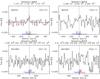 |
Fig. 4 IRAM-30 m spectra (Tmb) of the CO(1–0) (left) and CO(2–1) (right) lines at 115 GHz and 230 GHz, in Mrk 930 (top) and NGC 4861 (bottom). The spectra are rebinned to a common resolution of ~15 km s-1. Central velocities of [C ii], H i, and Hα, and their dispersions are also indicated in blue, green, and red, respectively. |
2.5. Herschel data: [C ii] and [O i]
The [C ii] 157μm and [O i] 63μm fine-structure cooling lines were observed in the six galaxies with the PACS spectrometer (Poglitsch et al. 2010) on board the Herschel Space Observatory (Pilbratt et al. 2010) as part of two Guaranteed Time Key Programs, the DGS (Madden et al. 2013) and SHINING (P.I. Sturm). The results of the full Herschel spectroscopic survey in dwarf galaxies is presented in Cormier et al. (in prep.). The PACS array is composed of 5 × 5 spatial pixels of size 9.4′′ each, covering a field-of-view of 47′′ × 47′′. The [C ii] observations consist of a 5 × 2 raster map for NGC 4861, and of 2 × 2 raster maps for the other galaxies. The [O i] observations consist of a 3 × 3 raster map for Mrk 1089, 2 × 2 raster maps for Haro 11 and UM 311, and single pointings for Mrk 930, NGC 625, NGC 4861. All observations were done in chop-nod mode with a chop throw of 6′ off the source (free of emission). The beam sizes are ~9.5′′ and 11.5′′, and the spectral resolution ~90 km s-1 and 240 km s-1 at 60μm and 160 μm, respectively (PACS Observer’s Manual 2011).
The data were reduced with the Herschel Interactive Processing Environment User Release v9.1.0 (Ott 2010), using standard scripts of the PACS spectrometer pipeline, and analyzed with the in-house software PACSman v3.52 (Lebouteiller et al. 2012). For the line fitting, the signal from each spatial position of the PACS array is fit with a second-order polynomial plus Gaussian for the baseline and line. The rasters are combined by drizzling to produce final maps of 3′′ pixel size.
The line intensity maps of [C ii] 157μm are displayed in Fig. 5. The [C ii] emission is extended in NGC 625, NGC 4861, and UM 311, and marginally in Haro 11, Mrk 1089, and Mrk 930. The [O i] emission is relatively more compact. The signal-to-noise ratio is ≥15σ on the peak of emission for both [C ii] and [O i]. We measure line fluxes both from the area covered by the maps and in a circular aperture of size that of the CO(1–0) beam (Table 3). The uncertainties come from the noise and from fitting the spectra. Calibration errors add an additional ~30% systematic uncertainty (Poglitsch et al. 2010) and thus dominate the total uncertainties.
2.6. Spitzer/IRS data: warm H2
All galaxies were observed with the Infrared Spectrograph (IRS; Houck et al. 2004) onboard the Spitzer Space Telescope (Werner et al. 2004), but H2 rotational lines are clearly seen in the spectra of Haro 11 and NGC 625 only, so we present the IRS data of these two galaxies. NGC 625 was observed on July 11, 2005 (P.I. Gehrz; AORKey 5051904) in staring mode with the high-resolution modules SH (≈10–20 μm; slit size 4.7′′ × 11.3′′) and LH (≈19–37 μm; slit size 11.1′′ × 22.3′′). The observation points toward the coordinates (RA, Dec) = (1h35m06.8s, –41d26m13s), where the [C ii] emission peaks. The processing of the Haro 11 observations is described in Cormier et al. (2012).
The data reduction and analysis were performed with SMART v8.2.2 (Lebouteiller et al. 2010; Higdon et al. 2004). IRS high-resolution observations are strongly affected by bad pixels in the detectors. Lacking the observation of an offset field for NGC 625 (and Haro 11), the quality of the spectra mainly relies on the pixel-cleaning step (performed with IRSCLEAN6) and on the comparison of the two spectra obtained at the two nod positions. The high-resolution spectra were obtained from the full-slit extraction, assuming both point-like and extended source calibrations, since NGC 625 is extended in the MIR bands while the H2 emission seems to be dominated by one knot.
We applied a first-order polynomial function fit to the baseline and a Gaussian profile to fit the line. We also added 10% of the line flux to the total uncertainties in order to take calibration uncertainties into account. The SH spectrum was multiplied by a factor 1.4 and 2 for the point-like and extended calibrations, respectively, to match the continuum level of the LH spectrum (larger aperture). Final fluxes were taken as the average of the fluxes obtained with the two nods and two different calibrations. The IRS observation of NGC 625 points toward the main starburst region where the [C ii] and IR peaks are located, east of the location of the CO(2–1) and CO(3–2) pointings (see the IRS footprint on Fig. 1). The IRS slit captures most, but probably not all, of the H2 emission since NGC 625 is extended in the Spitzer and Herschel broad bands. To estimate the total flux (over the entire galaxy), we scaled the H2 emission to that of the total 24μm Spitzer/MIPS emission (Bendo et al. 2012), multiplying all line fluxes by another factor 1.5. Individual spectra of the H2 lines are displayed in Fig. 6, and the line fluxes are given in Table 4. For Haro 11, we used the fluxes from Cormier et al. (2012) but re-estimated a more robust upper limit on the S(0) line by considering 3 × rms × FWHMinst/ sqrt(nres), where nres is the number of resolution elements in the instrumental FWHM.
 |
Fig. 5 Herschel/PACS [C ii] 157μm intensity maps (units of W m-2 sr-1). The PACS beam is indicated in blue (~11.5′′) and the CO(1–0) aperture used to integrate the flux in red. For NGC 625, the aperture is not centered on the [C ii] peak but on the same region covered by the CO(2–1) and CO(3–2) observations. The yellow contours show the area mapped in the [O i] 63μm line by PACS. |
Herschel/PACS [C ii] 157μm line observations and fluxes.
 |
Fig. 6 Spitzer/IRS spectra of the H2 lines at 9.66, 12.28, 17.04, and 28.22μm in NGC 625 (top row) and Haro 11 (bottom row). The red curve indicates the fit to the line when detected. |
The H2 S(1) 17.03μm and S(2) 12.28μm lines are detected in NGC 625 (Table 4), while we measure only an upper limit for the S(0) 28.22μm line, and the S(3) 9.66μm line falls outside of the observed wavelength range. The total luminosity of the two detected H2 lines is LH2 = 1.2 × 10⁴L⊙ for NGC 625. In the IRS spectrum of Haro 11, the S(1), S(2), and S(3) lines are detected, while the S(0) line is undetected. The total luminosity of the three detected lines is LH2 = 8.6 × 10⁶L⊙.
3. Analysis of the CO observations
3.1. Line profiles and velocities
We show the observed CO line profiles in Figs. 2 to 4. For comparison, we indicate below each CO spectrum the line centers of other relevant tracers: Hα, H i, and [C ii], as well as the velocity dispersion, when known. This dispersion measure includes broadening due to line fitting uncertainties (typically a few km s-1) and the instrumental line width (240 km s-1 for [C ii] with Herschel/PACS), which could blend several emission components. In those cases where mapped observations are available from the literature, we also include the range of observed peak positions across the source in the dispersion measure. Typical errors on the CO line centers are of 5–10 km s-1. Hα velocity information is taken from the following references: James et al. (2013) for Haro 11, Rubin et al. (1990) for Mrk 1089, Pérez-Montero et al. (2011) for Mrk 930, Van Eymeren et al. (2009) for NGC 4861, Marlowe et al. (1997) for NGC 625, and Terlevich et al. (1991) for UM 311. H i velocity information is taken from MacHattie et al. (2014) for Haro 11, Williams et al. (1991) for Mrk 1089, Thuan et al. (1999) for Mrk 930, Van Eymeren et al. (2009) for NGC 4861, Cannon et al. (2004) for NGC 625, and Smoker et al. (2000) for UM 311.
For Haro 11, we observe shifts in the velocity centers of the different tracers that could be due to the fact that the peak emission regions for atoms/ions and molecules are not cospatial. Sandberg et al. (2013) find a blueshift of ~44 km s-1 of the neutral gas relative to the ionized gas toward knot B and a redshift of ~32 km s-1 toward knot C. This indicates that the bulk of the cold gas emission could be associated with knot B. Interestingly, the PACS lines display rotation along the north-south axis and have broad profiles. The full width at half maximum (FWHM) of the FIR lines are larger than the PACS instrumental line widths. Subtracting the instrumental line width (240 km s-1 for [C ii] and 90 km s-1 for [O i] 63μm) quadratically, the intrinsic line width of [C ii] is ~160 km s-1, while those of [O iii] and [O i] are 250 and 140 km s-1, respectively, which is much larger than the CO line width of ~60 km s-1. The [O iii] broadening agrees with that of Hα, found as large as ~280 km s-1 by James et al. (2013). This confirms that the emission of the FIR lines arises from a larger region than the CO emission. The FIR lines are also too broad to be solely due to rotation and probably trace the presence of outflows.
For UM 311, important velocity shifts are observed for the different tracers, which are probably due to the crowding of the region, while for the other galaxies, CO and the other tracers peak at the same velocity overall. Mrk 1089 has broad CO profiles and the signal-to-noise is high enough in the APEX CO(2–1) and CO(3–2) spectra to clearly distinguish two velocity components, which are also present in the data from Leon et al. (1998). The spectral resolution of PACS does not allow us to resolve the separate narrow components seen in the CO profiles. Our [C ii] velocity map displays rotation, with redshifted emission east of the nucleus and blueshifted emission west of the nucleus. This agrees with the velocity analysis of H i and Hα, although the velocity fields are more irregular in the HCG 31 complex as a whole. In NGC 625, the CO(1–0) spectra have a single CO component of width ~70 km s-1. This emission may not be cospatial with the one seen in the ancillary CO(2–1) and CO(3–2) spectra (see Sect. 2.2), which are narrower (Table 2). While Hα and [C ii] peak spatially where the current star formation episode is taking place and where we detect CO with Mopra, H i peaks ~300 pc east (Cannon et al. 2004), where the second peak of [C ii] is located and where the APEX and JCMT observations point.
To summarize, the CO line detections are consistent with the velocities as obtained from Hα, H i, and [C ii]. Moreover, for a given galaxy, the different CO transitions exhibit the same line center and width (except CO(1–0) in NGC 625) within the uncertainties, showing that they come from the same component. This allows us to study CO line ratios (Sect. 4.1.1).
Spitzer/IRS H2 observations and fluxes.
3.2. Estimating the total CO emission
One of the complications in analyzing the various CO observations is the difference in beam sizes used for each transition. A larger beam may encompass more molecular clouds than probed by a smaller beam and thus hamper the comparison of the transitions with each other. A further complication stems from the possibility of CO emission outside the observed area if the galaxy is more extended than any of the beams, which influences the results when comparing CO properties to global properties (e.g., H i mass). Here we investigate how using different beam sizes affects the derived intensities.
 |
Fig. 7 Herschel PACS 100μm maps of NGC 4861 (left), NGC 625 (middle), and UM 311 (right), with the CO beams (Mopra in green, APEX in red, IRAM in blue, and the JCMT in yellow; see Fig. 1 for details). |
We have a complete coverage of the 100μm dust emission from Herschel for each galaxy at our disposal (Fig. 7; Rémy-Ruyer et al. 2013). If we assume that the distribution of the CO emission follows that of the 100μm dust continuum, we can roughly estimate the fraction of CO emission measured in each CO beam relative to the total CO emission. In principle, one should first subtract the H i column density for such approach. Here, we just assume a flat H i distribution. The spatial correlation between CO and the dust may not follow the same distribution on small scales in the Galaxy, but on larger scales in external galaxies, observations show a correlation between CO and IR emission (e.g., Tacconi & Young 1987; Sanders et al. 1991). The dust emission in the spectral energy distribution (SED) of our dwarf galaxies typically peaks between 70–100μm, which makes the 100μm emission a relatively good proxy for the dust column density. We convolve the 100μm maps with a 2D Gaussian. The position and width of the Gaussian are chosen to correspond to the position and width7 of the respective CO observations. The CO fractions that we estimate this way are listed in Table 5.
For Haro 11, Mrk 1089, and Mrk 930, we have recovered the bulk of the CO emission, and the CO luminosities that we report in Table 2 can be considered as total values. The fractions of the CO emission captured in the different CO beams agree within 20%, and comparing the CO intensities from one transition with another should be quite reliable (except for Mrk 930 but we only have a limit on its ratio). On the other hand, NGC 4861, NGC 625, and UM 311 are more extended and have complex shapes, and a large fraction of the total 100μm flux is emitted outside the CO beams. For these galaxies, we apply correction factors to the observed CO fluxes to estimate the total CO fluxes (Table 2). For NGC 4861, in which we targeted only the main H ii region, this correction factor is 3.5. For UM 311, the correction factor is 5 because of 100μm contamination from the two neighboring spiral galaxies. In this case, it is unclear whether the 100μm emission can be used to calculate beam correction factors since these systems may or may not be hosting CO clumps. For the sake of consistency, we apply this correction factor and estimate the total CO emission for the entire system. The CO line ratios are also uncertain by a factor of ~2. For NGC 625, we consider a single Mopra beam at the position of the CO(3–2) pointing. The difference between the 100μm fluxes integrated within the individual CO(1–0) and CO(3–2) beams is a factor of 2. The reason for this difference in NGC 625 is that the CO(3–2) observation does not point toward the peak of dust emission, and the CO(1–0) and CO(3–2) beam sizes are quite different. For the total CO emission of NGC 625, we consider the emission in all the CO(1–0) Mopra pointings, which cover the full extent of the galaxy seen in the dust continuum. When doing so, only 10% of the 100μm emission is emitted outside our CO(1–0) coverage.
These rough estimates of possible CO emission outside of the respective CO beams show that there are uncertainties of about a factor of 2 when comparing CO lines with each other, and a factor of ~3 for NGC 4861 and UM 311 when considering global quantities, such as molecular masses.
Estimated CO fractions (in %).
CO line ratios.
4. Physical conditions in the molecular clouds
In this section, we investigate the conditions (temperature, density, mass) characterizing the CO-emitting gas in our galaxies. First we discuss line ratios and derive total molecular masses using two values of the CO-to-H2 conversion factor (Galactic and metallicity-scaled) and dust measurements. Then we compare the observations with the predictions of the code RADEX and contrast our CO results with the analysis of the warm H2 gas.
H2 masses using CO observations, dust measurements, and models.
4.1. Empirical diagnostics
4.1.1. Line ratios
CO line intensity ratios give an insight into the conditions of the gas. Typical ratios are CO(2–1)/CO(1–0) ~ 0.8 and CO(3–2)/CO(1–0) ~ 0.6 in nearby spiral galaxies (Leroy et al. 2008; Wilson et al. 2009; Warren et al. 2010), and CO(3–2)/CO(2–1) ~ 0.8 in Galactic giant molecular clouds (Wilson et al. 1999). In blue compact dwarf galaxies, Sage et al. (1992) find an average ratio of CO(2–1)/CO(1–0) ~ 0.8, and Meier et al. (2001) derive an average CO(3–2)/CO(1–0) ratio of 0.6 in starburst dwarf galaxies. Ratios of CO(2–1)/CO(1–0) ≥1 are found in several starbursting compact dwarfs (e.g., Israel 2005) and bright regions of the Magellanic Clouds (Bolatto et al. 2000, 2003), and are usually attributed to the emission arising from smaller, warmer clumps, where CO(1–0) may not trace the total molecular gas.
The line ratios are calculated from the observed CO line intensities ICO (K km s-1), and solid angles of the source (Ωsource) and of the beam (Ωbeam), following Meier et al. (2001): 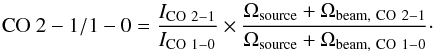 (2)The source sizes are unknown since we do not resolve individual molecular clouds. The assumed spatial distribution of the emission influences the derived CO line ratios (see also Sect. 3.2). Therefore we derive line ratios in two cases: (1) if the source is point-like (Ωsource ≪ Ωbeam) or (2) if the source is much larger than the beam (Ωbeam ≪ Ωsource). The latter case also applies if the source is not resolved but the CO emission comes from small clumps scattered across the beam and fills the beam (no beam dilution). Values of the line ratios are summarized in Table 6.
For the sample, we find an average CO(3–2)/CO(2–1) ratio of ~0.6 (measured on the detections only). Ratios of CO(3–2)/CO(1–0) and CO(2–1)/CO(1–0) are respectively ≥0.2 and ≥0.6 across the sample. Although there can be significant uncertainties due to the different beam sizes (see Sect. 3.2) and unknown source distribution, overall, we find no evidence for significantly different CO line ratios in our sample compared to normal-metallicity environments. Unlike resolved low-metallicity environments where CO line ratios can be high due to locally warmer gas temperatures, the line ratios (hence CO temperature) in our compact dwarf galaxies are moderate.
4.1.2. Molecular gas mass from CO observations
The molecular gas mass is usually derived from CO observations as a tracer of the cold H2 using the CO-to-H2 conversion factor XCO8, which relates the observed CO intensity to the column density of H2: ![\begin{equation} X_{\rm CO} = N({\rm H_2})/I_{\rm CO}~\rm{[cm^{-2}~(K~km~s^{-1})^{-1}]}. \end{equation}](/articles/aa/full_html/2014/04/aa22096-13/aa22096-13-eq191.png) (3)The extent to which the conversion from CO emission to cold H2 reservoir is affected by metallicity depends crucially on the relative proportion of H2 residing at moderate AV compared to the amount of enshrouded molecular gas. Even though both simulations and observations support a change in the CO-to-H2 conversion factor at low metallicities, the exact dependence of XCO on metallicity is not empirically well-established. Many physical characteristics other than metallicity, such as the topology of the molecular clouds and the distribution of massive ionizing stars, are also at play. We refer the reader to Bolatto et al. (2013) for a review on the topic. Therefore we consider two cases: one where XCO is equal to the Galactic value XCO,gal, and one where XCO scales with metallicity (noted XCO,Z) following Schruba et al. (2012), XCO,Z ∝ Z-2. Although the XCO conversion factor is calibrated for the CO(1–0) transition, we also estimate the molecular mass from the CO(2–1) and CO(3–2) observations, using the values of 0.8 and 0.6 for the CO(2–1)/CO(1–0) and CO(3–2)/CO(1–0) ratios respectively (Sect. 4.1.1). For each CO transition, the source size is taken as its corresponding beam size. For galaxies observed with IRAM (Mrk 930 and NGC 4861), we assume the source size to be that of the CO(1–0) beam since only the CO(1–0) observations in Mrk 930 leads to a detection. The resulting molecular gas masses of the six galaxies are reported in Table 7.
(3)The extent to which the conversion from CO emission to cold H2 reservoir is affected by metallicity depends crucially on the relative proportion of H2 residing at moderate AV compared to the amount of enshrouded molecular gas. Even though both simulations and observations support a change in the CO-to-H2 conversion factor at low metallicities, the exact dependence of XCO on metallicity is not empirically well-established. Many physical characteristics other than metallicity, such as the topology of the molecular clouds and the distribution of massive ionizing stars, are also at play. We refer the reader to Bolatto et al. (2013) for a review on the topic. Therefore we consider two cases: one where XCO is equal to the Galactic value XCO,gal, and one where XCO scales with metallicity (noted XCO,Z) following Schruba et al. (2012), XCO,Z ∝ Z-2. Although the XCO conversion factor is calibrated for the CO(1–0) transition, we also estimate the molecular mass from the CO(2–1) and CO(3–2) observations, using the values of 0.8 and 0.6 for the CO(2–1)/CO(1–0) and CO(3–2)/CO(1–0) ratios respectively (Sect. 4.1.1). For each CO transition, the source size is taken as its corresponding beam size. For galaxies observed with IRAM (Mrk 930 and NGC 4861), we assume the source size to be that of the CO(1–0) beam since only the CO(1–0) observations in Mrk 930 leads to a detection. The resulting molecular gas masses of the six galaxies are reported in Table 7.
For Haro 11, our CO detections yield a molecular gas mass of M(H2) ≃ 2.5 × 10⁸M⊙ (with XCO,gal). This value is higher than the previous upper limit of Bergvall et al. (2000), where they estimated M(H2) ≤ 108M⊙. For Mrk 1089, Leon et al. (1998) found M(H2) = 4.4 × 10⁸M⊙, This value is 1.5 times higher than what we derive with XCO,gal due to a beam (hence assumed source size) difference, and is below the value that we derive with XCO,Z. There are no other molecular mass estimates for Mrk 930, NGC 625, NGC 4861, and UM 311 in the literature to which we can compare our estimates. The molecular gas masses that we find with XCO,gal (denoted M(H2,gal)) are particularly low compared to, e.g., the IR luminosity or H i reservoir of our galaxies. We find an average ratio (with minimum and maximum values) of M(H2,gal)/M(Hi) ~ 12  % and M(H
 % (typically 10% in isolated galaxies; Solomon & Sage 1988). This stresses how deficient our galaxies are in CO.
4.1.3. Molecular gas mass from dust measurements
Other methods based on dust measurements are also used to quantify the total H2 gas, assuming that the gas mass is proportional to the dust mass via a fixed dust-to-gas mass ratio (e.g., Leroy et al. 2011; Sandstrom et al. 2013): ![\begin{equation} M{\rm (H}_2)~=~M_{\rm dust} \times \rm [{\it D/G}]^{-1}~-~[{\it M}(HI)+{\it M}(HII)]. \end{equation}](/articles/aa/full_html/2014/04/aa22096-13/aa22096-13-eq203.png) (4)We consider quantities within apertures defined from the dust emission and use aperture-corrected H i masses from Rémy-Ruyer et al. 2014 (Table 9). Except for Haro 11 (H ii mass from Cormier et al. 2012), we ignore M(H ii) from the equation since there is no ionized gas mass reported in the literature for our galaxies. We note that M(H ii) might be negligible in normal galaxies but might contribute more to the mass budget of dwarf galaxies. For the dust-to-gas mass ratio (D/G), we choose a D/G that scales linearly with metallicity (e.g., Edmunds 2001) and adopt the value D/G = 1/150 for O/H = 8.7 (Zubko et al. 2004). The dust masses are measured in Rémy-Ruyer et al. (in prep.) from a full dust SED modeling (Galliano et al. 2011) up to 500μm with Galactic dust opacities. Rémy-Ruyer et al. (in prep.) show that the thus derived dust masses are not significantly affected by the presence of a possible submm excess. Uncertainties on the dust masses due to the submm excess or a change of grain properties in low-metallicity environments are a factor 2–3 (Galametz et al. 2011; Galliano et al. 2011). We provide the D/G and dust masses in Table 8 and the derived H2 masses in Table 7. We find that the H2 masses resulting from this method are systematically higher by one or two orders of magnitude (except in Mrk 1089) than those determined from CO and XCO,gal.
(4)We consider quantities within apertures defined from the dust emission and use aperture-corrected H i masses from Rémy-Ruyer et al. 2014 (Table 9). Except for Haro 11 (H ii mass from Cormier et al. 2012), we ignore M(H ii) from the equation since there is no ionized gas mass reported in the literature for our galaxies. We note that M(H ii) might be negligible in normal galaxies but might contribute more to the mass budget of dwarf galaxies. For the dust-to-gas mass ratio (D/G), we choose a D/G that scales linearly with metallicity (e.g., Edmunds 2001) and adopt the value D/G = 1/150 for O/H = 8.7 (Zubko et al. 2004). The dust masses are measured in Rémy-Ruyer et al. (in prep.) from a full dust SED modeling (Galliano et al. 2011) up to 500μm with Galactic dust opacities. Rémy-Ruyer et al. (in prep.) show that the thus derived dust masses are not significantly affected by the presence of a possible submm excess. Uncertainties on the dust masses due to the submm excess or a change of grain properties in low-metallicity environments are a factor 2–3 (Galametz et al. 2011; Galliano et al. 2011). We provide the D/G and dust masses in Table 8 and the derived H2 masses in Table 7. We find that the H2 masses resulting from this method are systematically higher by one or two orders of magnitude (except in Mrk 1089) than those determined from CO and XCO,gal.
Dust-derived XCO factors.
If we assume that the H2 mass derived from the dust method is the true molecular mass, we can use the observed CO intensities and calculate the corresponding XCO value, XCO,dust. Since the full extent of the CO emission is unknown for the extended galaxies, we consider the fraction of the H2 mass that would fall in the CO(1–0) beam (Sect. 3.2). We re-estimate the CO(1–0) intensities based on the average H2 masses of the three CO transitions (Table 7) to derive XCO,dust (Table 8). The XCO,dust values are 10-50 times higher than XCO,gal, and sometimes even higher than XCO,Z. They scale with metallicity with power-law index ≃− 2.7: XCO,dust ∝ (O/H)-2.7. This relation with metallicity is steeper than what is found in Leroy et al. (2011) for Local Group galaxies (index of − 1.7), and similar to the one found in Israel (2000) (index of − 2.5) and in Schruba et al. (2012) for their complete sample of dwarf galaxies (index of − 2.8).
The numbers from this method are only given as an indication since they bear large uncertainties. We have done the same exercise on seven additional compact galaxies of the DGS (names in Table 9). These galaxies have 7.75 < O/H and are selected with total detected CO emission (within 50%, comparing the [C ii] emission inside and outside the CO aperture, Cormier et al., in prep.). However, the total gas masses predicted from the dust are often lower than the H i masses (and not only for the lowest metallicity objects). This shows the limitation of this method for compact low-metallicity galaxies that are H i-dominated and for which the D/G scales more steeply than linearly with metallicity, although its value is strongly variable because it depends on the star formation history of each individual galaxy (Rémy-Ruyer et al. 2014).
To conclude, the use of different methods (XCO,gal, XCO,Z, or dust) to measure the molecular gas reservoir in our galaxies results in very different mass estimates. This highlights the large uncertainties when using one method or the other. XCO,gal gives very low molecular gas masses that probably underestimate the true H2 gas in these low-metallicity galaxies. More realistic molecular masses (accounting for a CO-dark reservoir) are obtained with higher conversion factors from the dust method or from the scaling of XCO with metallicity.
Parameters for the star formation law.
4.2. Modeling of the CO emission with RADEX
We use the non-LTE code RADEX (Van der Tak et al. 2007) to analyze the physical conditions of the low-J CO-emitting gas. RADEX predicts the expected line intensity of a molecular cloud defined by constant column density (N(12CO)), gas density (nH2), and kinetic temperature (Tkin). In Fig. 8, we draw contour plots of CO line ratios for Mrk 1089 (similar plots are obtained for Haro 11, NGC 625, and UM 311) in the nH2–Tkin space for a given value of N(12CO) = 3 × 1015 cm-2 (typical of subsolar metallicity clouds; Shetty et al. 2011). The behavior of each line ratio we considered is similar in the nH2–Tkin space and relatively insensitive to N(12CO). Given the small number of observational constraints, no precise estimate of the physical conditions of the gas can be reached, except that Tkin ≥ 10 K. To break the degeneracy shown in Fig. 8, and particularly constrain the gas column density better, one would need optically thin line diagnostics with, e.g., 13CO measurements. When 13CO measurements are available, however, they usually preclude models with only a single molecular gas phase, and require at least two different phases (Meier et al. 2001; Israel 2005).
 |
Fig. 8 Results from RADEX for Mrk 1089: contour plot in kinetic temperature (Tkin)–density (nH2) parameter space (logarithmic scale), for a column density of N(12CO) = 3 × 1015 cm-2. The colored lines correspond to the observed line ratios of CO(2–1)/CO(1–0) (red), CO(3–2)/CO(1–0) (green), and CO(3–2)/CO(2–1) (orange), for both uniform filling (dash-dotted) and point-like (plain) limits. |
4.3. Excitation diagrams of the H2 molecule
Rotational transitions of molecular hydrogen are visible in the MIR with Spitzer and originate in a warm gas phase (temperature greater than a few hundred K), therefore putting constraints on the PDR properties of star-forming regions (and in particular the mass) rather than the cold molecular phase (e.g, Kaufman et al. 2006). As a first step in characterizing the conditions of the PDR, we assume local thermal equilibrium (LTE) and build an excitation diagram to derive the population of the H2 levels and estimate the temperature, column density, and mass of the warm molecular gas. We conduct this analysis only for the two galaxies Haro 11 and NGC 625, which have H2 lines detected in their IRS spectra. We consider the total fluxes in Table 4. The H2 emission is assumed to be optically thin. This approximation is justified by the fact that low-metallicity galaxies have, on average, lower AV, and clumpy material of high optical depth, while the warm H2 should arise from regions with larger filling factors. Also, the effects of extinction on the MIR H2 lines are not important in normal galaxies (Roussel et al. 2007) and ULIRGs (Higdon et al. 2006). We follow the method from Roussel et al. (2007), and assume a single temperature to match the S(1) to S(3) lines. This choice is biased toward higher temperatures (and lower masses) due to not detecting the S(0) line, as mentioned in Higdon et al. (2006) and Roussel et al. (2007). The source sizes are taken as the CO(1–0) Mopra coverage. The excitation diagrams are shown in Fig. 9. On the y axis, the observed intensities are converted to column densities in the upper levels Nu normalized by the statistical weights gu.
For Haro 11 (left panel), the best fit to the S(1), S(2), and S(3) lines agrees with a temperature of 350 K and column density of 1.1 × 1018 cm-2. The resulting H2 mass is M(H2) > 3.6 × 10⁶M⊙, which can be regarded as a lower limit since the S(0) line is not detected, hence not used as a constraint. Fitting the 1σ limit on the S(0) line and the S(1) line agrees with a temperature of 100 K and column density of 7.5 × 1019 cm-2. This yields an upper limit of M(H2) = 2.4 × 10⁸ M⊙. The exact warm molecular gas mass is therefore in between the two limits: 3.6 × 10⁶M⊙<M(H2,warm) < 2.4 × 10⁸ M⊙. For NGC 625 (right panel), the fit to the S(1) and S(2) lines yields a temperature of 380 K, and a column density of 2.7 × 1017 cm-2. This results in a lower limit on the mass of M(H2) > 5.8 × 10³ M⊙. Fitting the 1σ limit on the S(0) line and the S(1) line agrees with a temperature of 120 K and column density of 2.6 × 1019 cm-2. This gives a warm H2 mass of M(H2) < 5.7 × 10⁵ M⊙.
The limits that we obtain on M(H2,warm) indicate that the warm molecular gas mass in Haro 11 and NGC 625 is lower than their cold gas mass (Table 7). Roussel et al. (2007) find an average warm-to-cold ratio of M(H2,warm) /M(H2,cold) ~ 10% in star-forming galaxies. The temperatures and column densities of the warm H2 gas that we find are generally consistent with previous studies of nearby galaxies. In BCDs, Hunt et al. (2010) find an average temperature for the warm gas of ~245 K, and of ~100 K for Mrk 996, which is their only galaxy detected in the S(0) transition. However, their column densities are somewhat higher (N(H2) ~ 3 × 1021 cm-2) than ours. In more metal-rich galaxies, Roussel et al. (2007) find a median temperature of ~150 K for the colder H2 component (fitting the S(0) transition) and a temperature ≥400 K for the warmer component. Their column densities (N(H2) ~ 2 × 1020 cm-2) are in better agreement with ours.
 |
Fig. 9 Excitation diagrams of the S(0) to S(3) rotational H2 lines for Haro 11 (left) and NGC 625 (right). The Nu/gu ratios are normalized by the S(1) transition. The observations are shown with filled circles. The dotted lines indicate the best fit to the S(1) to S(3) transitions. The dashed line indicates the fit to the S(0) 1σ limit (open circle) and the S(1) transition. |
5. Full radiative transfer modeling of Haro 11
In this section, we investigate a radiative transfer model of Haro 11 using the spectral synthesis code Cloudy v13.01 (Ferland et al. 2013; Abel et al. 2005), for a more complete picture of the conditions in the PDR and molecular cloud. Cormier et al. (2012) analyzed the emission of ~17 MIR and FIR fine-structure lines from Spitzer and Herschel in Haro 11 with Cloudy. The model consists of a starburst surrounded by a spherical cloud. It first solves for the photoionized gas, which is constrained by six ionic lines, and then for the PDR, which is constrained by the FIR [O i] lines, assuming pressure equilibrium between the phases. A Galactic grain composition with enhanced abundance of small size grains, as often found in dwarf galaxies, is adopted (see Cormier et al. 2012 for details). We extend this model in light of the molecular data presented.
5.1. PDR properties
The PDR model of Cormier et al. (2012) is described by a covering factor ~10% and parameters nH = 105.1 cm-3, G0 = 103 Habing. This model is stopped at a visual extinction AV of 3 mag, just before CO starts to form, to quantify the amount of dark gas untraced by CO, and because no CO detections had been reported before. The emission of the Spitzer warm H2 lines is produced by this PDR, which has an average temperature of ~200 K. The total gas mass of the PDR derived with the model is M(PDR) = 1.2 × 10⁸M⊙ (Cormier et al. 2012) and is mainly molecular: 90% is in the form of H2 (dark gas component), and only 10% in the form of H i. This molecular gas originates in a warm phase, and its mass falls in between the limits on the warm molecular gas mass set in Sect. 4.3. The H i mass of the PDR is lower than the Bergvall et al. (2000) limit, which was the value adopted in Cormier et al. (2012). Thus the higher H i mass found by MacHattie et al. (2014) would not affect our PDR model but rather the diffuse ionized/neutral model component of Cormier et al. (2012).
We find that the intensity of the H2 S(1) transition is reproduced by the model within 10%, while the intensities of the S(2) and S(3) transitions are underpredicted by a factor of two. The S(0) prediction is below its upper limit. PDR models indicate that the H2 observations and, particularly, the S(2)/S(1) (0.6) and S(3)/S(1) (0.7) ratios could be better matched if another PDR phase of higher density or lower radiation field were considered. However, other factors such as uncertainties in the excitation physics of H2, along with uncertainties in UV and density, can also play a role (Kaufman et al. 2006). Reproducing lines coming from J> 3 have inherent uncertainties in the microphysics, and inconsistencies can arise from trying to simultaneously reproduce these lines at the same time as reproducing [C ii] and [O i].
5.2. Molecular cloud properties
To model the molecular cloud (AV ≥ 3 mag, where CO starts to form) with Cloudy, we continue the PDR model described above to larger AV. This way, we assume that the observed CO emission is linked to the densest star-forming cores rather than to a diffuse phase. Since we have no observations of molecular optically thin tracers or denser gas tracers than CO, we use the cold dust emission to set our stopping criterion for the models and determine the AV appropriate to reproduce the FIR/submm emission of the spectral energy distribution of Haro 11. We find that the Herschel PACS and SPIRE photometry is best reproduced (within 30%) for AV ~ 30 mag, and we take this value as our stopping criterion.
 |
Fig. 10 Cloudy model predictions for the CO line luminosities as a function of AV. The models are stopped at AV of 30 mag, and the covering factor is set to ~5%. Observations of the CO(1–0) (upper limit), CO(2–1), and CO(3–2) lines are represented by filled circles on the right-hand side of the plots. Top: no turbulent velocity included. Bottom: including a turbulent velocity uturb of 30 km s-1. |
We find that the CO emission is essentially produced at 3 <AV< 6 mag, where CO dominates the cooling of the gas. For larger AV, the gas temperature stabilizes around 30 K, and denser gas tracers such as HNC, CN, and CS take over the cooling. Densities in the molecular cloud reach 106.3 cm-3. For AV> 10 mag, ~30% of the carbon is in the form of CO, and the condensation of CO onto grain surfaces reaches ~10%. The photoelectric effect on grains is mostly responsible for the heating of the gas at the surface of the cloud, and grain collisions are the main heating source deeper into the cloud. Figure 10 (top) shows the Cloudy model predictions for the CO line luminosities (from CO(1–0) to CO(8–7)) as a function of AV (models are stopped at AV = 30 mag). The observed CO(2–1) and CO(3–2) luminosities are matched by this model within a factor of 2, and the CO(1–0) model prediction falls below the observed upper limit. The predicted CO(1–0) intensity is only three times lower than our observed upper limit, indicating that higher-performance telescopes (such as ALMA) should be able to detect this transition. The CO(3–2)/CO(2–1) ratio is overpredicted by a factor of 3 compared to the observed uniform-filling ratio.
The modeled total mass depends strongly on the assumed geometry and on the SED fitting, which has an additional complication due to an excess of submm emission (Galametz et al. 2011). We select two values of maximum AV, one at which the shielding is sufficient for CO to completely form and the SED is well fit (within 30%) up to 350 μm (AV,max1 = 15 mag), and one at which the SED is fit up to 500 μm (AV,max2 = 30 mag). The molecular gas masses corresponding to those AV are M(H2) = 7.2 × 10⁸M⊙ and M(H2) = 1.6 × 10⁹M⊙, respectively. We adopt the latter value in the rest of this paper, but recall that this mass estimate is uncertain by a factor of ~2. This is the mass in the molecular phase associated with CO emission. The molecular gas mass in the CO-dark PDR layer is then ~10% that of the CO-emitting core (Sect. 5.1), so the warm-to-cold molecular gas mass in Haro 11 is very close to the values found in Roussel et al. (2007). The total molecular mass in Haro 11 (CO-dark gas+CO core) is 1.7 × 10⁹M⊙, close to the value derived from XCO,Z. The resulting αCO,model is ~ 50 M⊙ (K km s-1 pc2)-1 and is about ten times αCO,gal = 4.3 M⊙ (K km s-1 pc2)-1. The total (H ii+H i+H2, including He) model gas mass is 3.3 × 10⁹M⊙, and the total gas mass to stellar mass (1010M⊙) ratio is ~35%. Despite active photodissociation and low CO luminosities, the overall molecular gas content of Haro 11 is not particularly low. The mass budget of Haro 11 is dominated by its molecular gas, followed by the ionized and neutral gas phases.
Modeling the molecular cloud to AV of 30 mag has implications on the model predictions for the lines coming from other media given the geometry adopted for the model. Even though the ionic lines are affected little, the PDR H2 lines can be subject to dust extinction, and the [O i] lines become optically thick, their emission being reduced by a factor of two at most. If true, then we would need an additional component in the model, another PDR phase or other excitation mechanisms, such as shocks (e.g., Hollenbach & McKee 1989) to reproduce the observations. Spatially resolved observations of, say, [C i] for the PDR, as well as optically thin molecular tracers, are needed to confirm this PDR/molecular structure.
5.3. Influence of micro-turbulence
We discuss the effects of adding a turbulent velocity in the Cloudy models, in particular to the predicted CO line ratios, which are sensitive to the temperature in the high-density regime. Turbulence may be an important factor in setting the ISM conditions in Haro 11 since it has been found to be dynamically unrelaxed (Östlin et al. 2001; James et al. 2013). The microphysical turbulence is linked to the observed CO FWHM (~60 km s-1) via 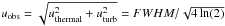 . Turbulence is included in the pressure balance, with the term
  , hence dissipating some energy away from the cloud.
We show the temperature profile in the cloud in Fig. 11 (top panel). We have chosen to display the results for a turbulent velocity of 30 km s-1 to illustrate the effect of turbulence on the profiles clearly. The gas temperature decreases more quickly with AV in the molecular cloud from 200 K down to 7 K, and stabilizes around 10 K in the CO-emitting region. The density stays around that of the PDR (105.2 cm-3), so similar results are found in the case of a constant density. Adding turbulence has a profound effect on the CO ladder, where high-J lines are emitted in a thinner region close to the cloud surface compared to low-J CO lines (Fig. 10, bottom). With turbulence, the low-J CO lines start to form at AV of 5–6 mag. The [C i] 370 and 610 μm lines are actually enhanced by an order of magnitude between AV of 2–5 mag, and then the lowest CO transitions (lowest Texc) are enhanced. As a consequence, ratios of CO(3–2)/CO(2–1) decrease with increasing turbulent velocity (Fig. 11, bottom). The observed CO(3–2)/CO(2–1) ratio is matched better by the models when including a turbulent velocity >10 km s-1. Observations of [C i] and higher-J (J> 4) CO lines would help validate the importance of turbulence and investigate possible excitation mechanisms in low-metallicity galaxies.
 |
Fig. 11 Top: temperature profile in the cloud. The dotted profile is without turbulence, and the plain profile with a turbulent velocity of 30 km s-1. The first vertical gray band indicates the transition into the molecular cloud (H2>H i), and the second gray band when CO starts to form. Bottom: cloudy model predictions for the CO(3–2)/CO(2–1) ratio as a function of turbulent velocity. The two cases of constant density (open symbols) and constant pressure (filled symbols) are considered. The horizontal dotted line indicates the observed CO ratio and the vertical dashed line the observed CO velocity |
6. Star formation and total gas reservoir
In this section, we analyze the global star formation properties of our low-metallicity galaxies and relate their gas reservoir to the star formation activity in order to contrast what we find for SFE when we use a tracer of a specific ISM phase as a proxy for the total gas reservoir.
6.1. [C ii], [O i], and CO
The [C ii]-to-CO(1–0) ratio can be used as a diagnostic of the star formation activity in nearby normal galaxies (Stacey et al. 1991) and high-redshift galaxies (z ~ 1–2; Stacey et al. 2010), with average values between 2000 and 6000 (for star-forming galaxies). High [C ii]/CO ratios are observed in low-metallicity dwarf galaxies (Madden 2000) because of the different cloud structure with smaller CO cores and larger PDR envelopes, and also because of increased photoelectric heating efficiencies in the PDR, caused by dilution of the UV radiation field that can enhance the [C ii] cooling (Israel & Maloney 2011). For our sample, we also find high ratios with [C ii]/CO(1–0) ≥ 7000 (Fig. 12, top left). This indicate that most of the gas is exposed to intense radiation fields and that the star-forming regions dominate the global emission of our galaxies.
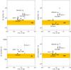 |
Fig. 12 [C ii] and [O i]-to-CO ratios versus 70 μm/100 μm. The horizontal orange band indicates the average ratio [C ii]/CO(1–0) of 2000–6000 observed in star-forming regions of the Galaxy and galaxies (Stacey et al. 1991). For the [C ii]/CO(3–2) horizontal band, a ratio R31 = 0.6 is considered. The blue circles correspond to the model predictions for Haro 11. |
C0 has an ionization potential of 11.26 eV, and critical densities of 50 cm-3 for collisions with electrons and of 3 × 103 cm-3 for collisions with hydrogen atoms. Thus, C+ can arise from the surface layers of PDRs but also from diffuse ionized gas, as well as diffuse neutral gas. In Fig. 12, we also show line ratios with [O i], which could be a more accurate tracer of the PDR envelope given the possible origins of the [C ii] emission, and with CO(3–2), for which we have more detections than CO(1–0). The [O i]/CO(1–0) ratios are generally lower than the [C ii]/CO(1–0) ratios because of the high [C ii]/[O i] ratios found in our dwarf galaxies. However, the ratios remain high when using [O i]. Although there are only four data points, the scatter in the [C ii]/CO(3–2) values is slightly reduced. The color ratio of 70 μm/100 μm is an indicator of the dust temperature and thus of the relative contribution of the H ii region and PDR to the global emission. One might, therefore, expect higher line-to-CO ratios for higher 70 μm/100 μm ratios. We do not see a direct correlation between the observed line-to-CO ratios and 70 μm/100 μm color or metallicity, but maybe a slight increase of [C ii]/CO with 70μm/100μm.
6.2. Star formation law
We investigate how the different gas reservoirs of H i and H2 are related to the star formation activity measured in our galaxies, and compare them to the dataset of starburst and spiral galaxies from Kennicutt (1998), as well as the other compact dwarf galaxies from the DGS with CO(1–0) measurements. We look at the SFR surface density (ΣSFR) and gas surface density Σgas = ΣHI + ΣH2. For ΣSFR, we use the LTIR-derived SFRs from the formula of Murphy et al. (2011), divided by the source size, which is taken as the dust aperture from Rémy-Ruyer et al. (2013). For the hydrogen masses, we consider the H i within the dust apertures from Rémy-Ruyer et al. (2014), and the H2 derived from total CO intensities with XCO,gal, XCO,Z, and from dust measurements (Table 7) for our sample (Fig. 13), and with XCO,Z and CO intensities from the literature for the DGS galaxies (Fig. 14). Those galaxies have metallicities between 1/40 and 1 Z⊙ (Madden et al. 2013). We summarize those parameters in Table 9. The hydrogen masses are multiplied by a factor 1.36 in the figures to include helium.
 |
Fig. 13 Star formation rate surface density (ΣSFR) versus gas surface density (Σgas). Our dwarf galaxies are represented by filled circles, and the colors show the contribution from the separate observed phases. Cloudy models for Haro 11 correspond to the filled rectangles (Sect. 5.2). The starbursts and spirals from Kennicutt (1998) are represented by stars and triangles, respectively. The diagonal dotted line indicates a fit to the Schmidt-Kennicutt law, with power index 1.4 to starbursts and spirals (Kennicutt 1998). |
In Figs. 13 and 14, we see that most low-metallicity galaxies fall close to the Schmidt-Kennicutt relation. The less active galaxies are generally dominated by their H i gas, while some of the most active galaxies, such as Haro 11, are dominated by their H2 gas. Several galaxies stand farther to the right of the relation (I Zw 18, Mrk 209, NGC 4861, UM 461, VII Zw 403), hence appear either more gas-rich, with part of their H i gas probably less connected to the star formation activity, or more quiescent than expected, where the TIR luminosity might slightly underestimate the star formation rate (Kennicutt & Evans 2012). Mrk 209 shows a strikingly high molecular surface density, which would be an indication that it is on the verge of forming stars. However, it is known to already host young super star clusters and WR features (e.g., Thuan & Izotov 2005). Moreover, its warm molecular component inferred from Spitzer data is only ~ 6 × 10³M⊙ (Hunt et al. 2010), which is orders of magnitude lower than the estimated cold molecular gas. These indications combined probably mean that we are overestimating ΣH2 with the high conversion factor XCO,Z used (and because of uncertainties on the metallicity). Two galaxies (Haro 11 and, more moderately, NGC 5253), which have the highest ΣSFR, lie to the left of the standard Schmidt-Kennicutt relation, even when considering high XCO values. Both are active blue compact galaxies. The presence of young super star clusters in NGC 5253 and clear lack of CO suggest that the starburst was triggered by accretion of gas from outside the galaxy and formed with high efficiency (Meier et al. 2002). Haro 11 is also known to have undergone a merger event (Östlin et al. 1999) and behaves like starbursting mergers (Daddi et al. 2010). We note that the position of our low-metallicity galaxies coincide with the position of spiral galaxies on Fig. 14. We have used apertures that are large enough to encompass the total FIR continuum emission and are ≥1.5 × r25 (Rémy-Ruyer et al. 2013). If we were to zoom on the star-forming regions of our galaxies, those would generally move closer towards the position of the starburst galaxies.
The gas depletion time, i.e. the time needed to consume the existing gas reservoir given the SFR, is expressed as the inverse of the star formation efficiency: τdep = Σgas/ ΣSFR [yr]. In nearby, predominantly late-type disk galaxies, the average molecular depletion time found by Bigiel et al. (2008) is around 2 Gyr. For our sample, taking the cold H2 (XCO,Z) mass values from Table 7 and including helium, we get molecular depletion times of ~0.1 Gyr (for Haro 11) – 0.3 Gyr (for Mrk 930) up to 3 Gyr (for NGC 4861), and a median value of 0.7 Gyr for the compact DGS sample. Sage et al. (1992) find similarly low values (~0.1 Gyr) for their sample of BCDs, although they use relatively lower conversion factors, of two to three times XCO,gal. Therefore, even when using a metallicity-scaled XCO factor, we find that our systems have short molecular gas depletion times typical of interacting systems, starbursts, and ULIRGs.
If we are accounting for all the gas related to the star formation, such short depletion times indicate that our dwarf galaxies are efficient in forming stars. This can be understood by the fact that several super star clusters are observed in those galaxies, and BCGs do have higher cluster formation efficiencies than normal galaxies (Adamo et al. 2011a). If these galaxies keep forming stars at the current rate, they would consume all their gas quickly. Therefore they might be caught in a bursty episode (since they are selected as bright in the IR). When adding the H i data, the average total gas depletion time over the sample is τdep ~ 5 Gyr. This value is significantly higher than the molecular depletion times since most galaxies are H i-dominated. This H i gas may also play a role in regulating the star formation, as direct fuel at very low metallicities (Krumholz 2012) or as future fuel, since part of the H i we measure may be residing in the envelopes of the molecular clouds. Regardless of the role of the H i, the picture that emerges is a very rapid and efficient conversion of molecular gas into stars in low-metallicity dwarf galaxies.
7. Conclusions
The state and abundance of the molecular gas, observed through the molecule CO, is not well known in dwarf galaxies. To address this issue, we obtained new observations of the CO(1–0), CO(2–1), and CO(3–2) lines in a subsample of six low-metallicity galaxies of the Herschel Dwarf Galaxy Survey (Haro 11, Mrk 930, Mrk 1089, NGC 4861, NGC 625, and UM 311), which we combine with existing broad band and atomic fine-structure line observations. We summarize our results as follows.
-
Out of the six targets, five are detected in at least one CO transition, but NGC 4861 remains undetected in CO. Three of the targets, Haro 11, Mrk 930 (marginal detection), and UM 311, with metallicities Z ~ 1/3, 1/5, and 1/2 Z⊙ respectively, were never detected in CO before, and no CO data were reported in the literature for NGC 625.
-
CO is found to be faint in these six dwarf galaxies, especially relative to the [C ii] 157μm line, since we derive [C ii]/CO(1–0) ratios ≥7000. In particular, this hints at the low filling factor of the CO-emitting material and high photoelectric [C ii] heating efficiency, as previously suggested (Israel et al. 1996; Madden 2000).
-
Molecular gas mass estimates are quite uncertain and vary significantly depending on the method used (XCO, dust measurements, etc.). A Galactic conversion factor predicts unrealistically low masses, while the dust method, a metallicity-scaled XCO, or radiative transfer modeling predict higher molecular masses with low accuracy. Even when considering high XCO conversion factors for our sample of low-metallicity galaxies, the molecular content makes a small contribution to the total ISM mass budget compared to the H i gas (except for Haro 11).
-
We compared the star formation activity to the gas reservoir for a sample extended to the compact low-metallicity galaxies of the DGS. Despite their low molecular content, all galaxies are in relative agreement with the (total gas) Schmidt-Kennicutt relation. The BCGs NGC 5253 and Haro 11, which has a high molecular-to-atomic gas fraction, are exceptions and may be intrinsically more efficient at forming stars. Even with a metallicity-scaled XCO factor, the molecular gas depletion times of our low-metallicity galaxies are short. Our results imply either that 1) the molecular gas forms stars with a different efficiency in the dwarf galaxies of our sample than in normal spirals or 2) if a universal total (as opposed to molecular) gas depletion time applies, then the atomic and possibly the ionized gas are participating in star formation in those galaxies.
The solar metallicity is taken as (O/H)⊙ = 8.7 (Asplund et al. 2009).

Dame et al. (2001) report an average value in the Galaxy of XCO,gal = 1.8 × 1020 cm-2 (K km s-1)-1, and Fermi measurements give XCO,gal ≃ 2 × 1020 cm-2 (K km s-1)-1 for large-scale complexes (e.g., Ackermann et al. 2011). In the following, we adopt XCO,gal = 2 × 1020 cm-2 (K km s-1)-1. These variations in XCO,gal are insignificant here compared to the orders of magnitude variations that may prevail in our low-metallicity sample.
Acknowledgments
This research was supported by Sonderforschungsbereich SFB 881 “The Milky Way System” of the German Research Foundation (DFG), and by the Agence Nationale de la Recherche (ANR, France) through the programme SYMPATICO (Programme Blanc Projet ANR-11-BS56-0023). V.L. is supported by a CEA/Marie Curie Eurotalents fellowship. This research made use of the NASA/IPAC Extragalactic Database (NED), which is operated by the Jet Propulsion Laboratory, California Institute of Technology, under contract with the National Aeronautics and Space Administration. This work is based in part on observations made with the Spitzer Space Telescope, which is operated by the Jet Propulsion Laboratory, California Institute of Technology under a contract with NASA. The Mopra Radio Telescope is part of the Australia Telescope National Facility, which is funded by the Commonwealth of Australia for operation as a National Facility managed by CSIRO. The University of New South Wales Digital Filter Bank used for the observations with the Mopra Telescope was provided with support from the Australian Research Council. We thank the IRAM-30 m staff for their help with the observations. This publication is based on data acquired with the Atacama Pathfinder Experiment (APEX). APEX is a collaboration between the Max-Planck-Institut für Radioastronomie, the European Southern Observatory, and the Onsala Space Observatory.
References
- Abel, N. P., Ferland, G. J., Shaw, G., & van Hoof, P. A. M. 2005, ApJS, 161, 65 [NASA ADS] [CrossRef] [Google Scholar]
- Ackermann, M., Ajello, M., Baldini, L., et al. 2011, ApJ, 726, 81 [NASA ADS] [CrossRef] [Google Scholar]
- Adamo, A., Östlin, G., & Zackrisson, E. 2011a, MNRAS, 417, 1904 [NASA ADS] [CrossRef] [Google Scholar]
- Adamo, A., Östlin, G., Zackrisson, E., et al. 2011b, MNRAS, 415, 2388 [NASA ADS] [CrossRef] [Google Scholar]
- Albrecht, M., Chini, R., Krügel, E., Müller, S. A. H., & Lemke, R. 2004, A&A, 414, 141 [NASA ADS] [CrossRef] [EDP Sciences] [Google Scholar]
- Asplund, M., Grevesse, N., Sauval, A. J., & Scott, P. 2009, ARA&A, 47, 481 [NASA ADS] [CrossRef] [Google Scholar]
- Bayet, E., Gerin, M., Phillips, T. G., & Contursi, A. 2004, A&A, 427, 45 [NASA ADS] [CrossRef] [EDP Sciences] [Google Scholar]
- Bendo, G. J., Galliano, F., & Madden, S. C. 2012, MNRAS, 423, 197 [NASA ADS] [CrossRef] [Google Scholar]
- Bergvall, N., Masegosa, J., Östlin, G., & Cernicharo, J. 2000, A&A, 359, 41 [NASA ADS] [Google Scholar]
- Bigiel, F., Leroy, A., Walter, F., et al. 2008, AJ, 136, 2846 [NASA ADS] [CrossRef] [Google Scholar]
- Bigiel, F., Leroy, A. K., Walter, F., et al. 2011, ApJ, 730, L13 [NASA ADS] [CrossRef] [Google Scholar]
- Bolatto, A. D., Jackson, J. M., Israel, F. P., Zhang, X., & Kim, S. 2000, ApJ, 545, 234 [NASA ADS] [CrossRef] [Google Scholar]
- Bolatto, A. D., Leroy, A., Israel, F. P., & Jackson, J. M. 2003, ApJ, 595, 167 [NASA ADS] [CrossRef] [Google Scholar]
- Bolatto, A. D., Wolfire, M., & Leroy, A. K. 2013, ARA&A, 51, 207 [Google Scholar]
- Braine, J., Duc, P.-A., Lisenfeld, U., et al. 2001, A&A, 378, 51 [NASA ADS] [CrossRef] [EDP Sciences] [Google Scholar]
- Cannon, J. M. 2004, Ph.D. Thesis, University of Minnesota, USA [Google Scholar]
- Cannon, J. M., McClure-Griffiths, N. M., Skillman, E. D., & Côté, S. 2004, ApJ, 607, 274 [NASA ADS] [CrossRef] [Google Scholar]
- Cannon, J. M., Skillman, E. D., Sembach, K. R., & Bomans, D. J. 2005, ApJ, 618, 247 [NASA ADS] [CrossRef] [Google Scholar]
- Cormier, D., Madden, S. C., Hony, S., et al. 2010, A&A, 518, L57 [NASA ADS] [CrossRef] [EDP Sciences] [Google Scholar]
- Cormier, D., Lebouteiller, V., Madden, S. C., et al. 2012, A&A, 548, A20 [NASA ADS] [CrossRef] [EDP Sciences] [Google Scholar]
- Daddi, E., Elbaz, D., Walter, F., et al. 2010, ApJ, 714, L118 [Google Scholar]
- Dale, D. A., Helou, G., Contursi, A., Silbermann, N. A., & Kolhatkar, S. 2001, ApJ, 549, 215 [NASA ADS] [CrossRef] [Google Scholar]
- Dame, T. M., Hartmann, D., & Thaddeus, P. 2001, ApJ, 547, 792 [NASA ADS] [CrossRef] [Google Scholar]
- de Vaucouleurs, G., de Vaucouleurs, A., Corwin, Jr., H. G., et al. 1991, Third Reference Catalogue of Bright Galaxies, Volume I: Explanations and references, Volume II: Data for galaxies between 0h and 12h, Volume III: Data for galaxies between 12h and 24h (New York: Springer Verlag) [Google Scholar]
- Edmunds, M. G. 2001, MNRAS, 328, 223 [NASA ADS] [CrossRef] [Google Scholar]
- Elmegreen, B. G., Rubio, M., Hunter, D. A., et al. 2013, Nature, 495, 487 [NASA ADS] [CrossRef] [Google Scholar]
- Ferland, G. J., Porter, R. L., van Hoof, P. A. M., et al. 2013, Rev. Mex. Astron. Astrofis., 49, 137 [Google Scholar]
- Galametz, M., Madden, S., Galliano, F., et al. 2009, A&A, 508, 645 [NASA ADS] [CrossRef] [EDP Sciences] [Google Scholar]
- Galametz, M., Madden, S. C., Galliano, F., et al. 2011, A&A, 532, A56 [NASA ADS] [CrossRef] [EDP Sciences] [Google Scholar]
- Galliano, F., Hony, S., Bernard, J.-P., et al. 2011, A&A, 536, A88 [NASA ADS] [CrossRef] [EDP Sciences] [Google Scholar]
- Genzel, R., Tacconi, L. J., Combes, F., et al. 2012, ApJ, 746, 69 [NASA ADS] [CrossRef] [Google Scholar]
- Gil de Paz, A., Boissier, S., Madore, B. F., et al. 2007, ApJS, 173, 185 [NASA ADS] [CrossRef] [Google Scholar]
- Glover, S. C. O., & Clark, P. C. 2012, MNRAS, 421, 9 [NASA ADS] [Google Scholar]
- Glover, S. C. O., Federrath, C., Mac Low, M.-M., & Klessen, R. S. 2010, MNRAS, 404, 2 [NASA ADS] [Google Scholar]
- Grenier, I. A., Casandjian, J.-M., & Terrier, R. 2005, Science, 307, 1292 [NASA ADS] [CrossRef] [PubMed] [Google Scholar]
- Grimes, J. P., Heckman, T., Strickland, D., et al. 2007, ApJ, 668, 891 [NASA ADS] [CrossRef] [Google Scholar]
- Guseva, N. G., Izotov, Y. I., & Thuan, T. X. 1998, Kinem. Phys. Celest. Bodies, 14, 41 [Google Scholar]
- Hickson, P. 1982, ApJ, 255, 382 [NASA ADS] [CrossRef] [Google Scholar]
- Higdon, S. J. U., Devost, D., Higdon, J. L., et al. 2004, PASP, 116, 975 [NASA ADS] [CrossRef] [Google Scholar]
- Higdon, S. J. U., Armus, L., Higdon, J. L., Soifer, B. T., & Spoon, H. W. W. 2006, ApJ, 648, 323 [NASA ADS] [CrossRef] [Google Scholar]
- Hollenbach, D., & McKee, C. F. 1989, ApJ, 342, 306 [NASA ADS] [CrossRef] [Google Scholar]
- Hopkins, A. M., Schulte-Ladbeck, R. E., & Drozdovsky, I. O. 2002, AJ, 124, 862 [NASA ADS] [CrossRef] [Google Scholar]
- Houck, J. R., Roellig, T. L., Van Cleve, J., et al. 2004, in SPIE Proc. 5487, ed. J. C. Mather, 62 [Google Scholar]
- Hunt, L. K., Thuan, T. X., Izotov, Y. I., & Sauvage, M. 2010, ApJ, 712, 164 [NASA ADS] [CrossRef] [Google Scholar]
- Iglesias-Paramo, J., & Vilchez, J. M. 1997, ApJ, 479, 190 [NASA ADS] [CrossRef] [Google Scholar]
- Indebetouw, R., Brogan, C., Chen, C.-H. R., et al. 2013, ApJ, 774, 73 [NASA ADS] [CrossRef] [Google Scholar]
- Israel, F. 2000, in Molecular Hydrogen in Space, eds. F. Combes & G. Pineau des Fôrets (Cambridge: Cambridge University Press), 293 [Google Scholar]
- Israel, F. P. 2005, A&A, 438, 855 [NASA ADS] [CrossRef] [EDP Sciences] [Google Scholar]
- Israel, F. P., & Maloney, P. R. 2011, A&A, 531, A19 [NASA ADS] [CrossRef] [EDP Sciences] [Google Scholar]
- Israel, F. P., Tacconi, L. J., & Baas, F. 1995, A&A, 295, 599 [NASA ADS] [Google Scholar]
- Israel, F. P., Maloney, P. R., Geis, N., et al. 1996, ApJ, 465, 738 [NASA ADS] [CrossRef] [Google Scholar]
- Izotov, Y. I., & Thuan, T. X. 1998, ApJ, 500, 188 [NASA ADS] [CrossRef] [Google Scholar]
- James, B. L., Tsamis, Y. G., Walsh, J. R., Barlow, M. J., & Westmoquette, M. S. 2013, MNRAS, 430, 2097 [NASA ADS] [CrossRef] [Google Scholar]
- Kaufman, M. J., Wolfire, M. G., & Hollenbach, D. J. 2006, ApJ, 644, 283 [NASA ADS] [CrossRef] [Google Scholar]
- Kennicutt, Jr., R. C. 1998, ApJ, 498, 541 [NASA ADS] [CrossRef] [Google Scholar]
- Kennicutt, R. C., & Evans, N. J. 2012, ARA&A, 50, 531 [NASA ADS] [CrossRef] [Google Scholar]
- Kennicutt, Jr., R. C., Lee, J. C., Funes, S. J. J. G., Sakai, S., & Akiyama, S. 2008, ApJS, 178, 247 [NASA ADS] [CrossRef] [Google Scholar]
- Kester, D. J. M., Beintema, D. A., & Lutz, D. 2003, in The Calibration Legacy of the ISO Mission, eds. L. Metcalfe, A. Salama, S. B. Peschke, & M. F. Kessler, ESA SP, 481, 375 [Google Scholar]
- Kobulnicky, H. A., Dickey, J. M., Sargent, A. I., Hogg, D. E., & Conti, P. S. 1995, AJ, 110, 116 [NASA ADS] [CrossRef] [Google Scholar]
- Krumholz, M. R. 2012, ApJ, 759, 9 [NASA ADS] [CrossRef] [Google Scholar]
- Krumholz, M. R., Leroy, A. K., & McKee, C. F. 2011, ApJ, 731, 25 [NASA ADS] [CrossRef] [Google Scholar]
- Ladd, N., Purcell, C., Wong, T., & Robertson, S. 2005, PASA, 22, 62 [NASA ADS] [CrossRef] [Google Scholar]
- Lebouteiller, V., Bernard-Salas, J., Sloan, G. C., & Barry, D. J. 2010, PASP, 122, 231 [NASA ADS] [CrossRef] [Google Scholar]
- Lebouteiller, V., Cormier, D., Madden, S. C., et al. 2012, A&A, 548, A91 [NASA ADS] [CrossRef] [EDP Sciences] [Google Scholar]
- Lee, J. C., Gil de Paz, A., Kennicutt, Jr., R. C., et al. 2011, ApJS, 192, 6 [NASA ADS] [CrossRef] [Google Scholar]
- Leon, S., Combes, F., & Menon, T. K. 1998, A&A, 330, 37 [NASA ADS] [Google Scholar]
- Leroy, A., Bolatto, A. D., Simon, J. D., & Blitz, L. 2005, ApJ, 625, 763 [NASA ADS] [CrossRef] [Google Scholar]
- Leroy, A. K., Walter, F., Brinks, E., et al. 2008, AJ, 136, 2782 [NASA ADS] [CrossRef] [Google Scholar]
- Leroy, A. K., Walter, F., Bigiel, F., et al. 2009, AJ, 137, 4670 [NASA ADS] [CrossRef] [Google Scholar]
- Leroy, A. K., Bolatto, A., Gordon, K., et al. 2011, ApJ, 737, 12 [NASA ADS] [CrossRef] [Google Scholar]
- MacHattie, J. A., Irwin, J. A., Madden, S. C., Cormier, D., & Rémy-Ruyer, A. 2014, MNRAS, 438, L66 [NASA ADS] [CrossRef] [Google Scholar]
- Madden, S. C. 2000, New Astron. Rev., 44, 249 [NASA ADS] [CrossRef] [Google Scholar]
- Madden, S. C., Poglitsch, A., Geis, N., Stacey, G. J., & Townes, C. H. 1997, ApJ, 483, 200 [NASA ADS] [CrossRef] [MathSciNet] [Google Scholar]
- Madden, S. C., Rémy-Ruyer, A., Galametz, M., et al. 2013, PASP, 125, 600 [NASA ADS] [CrossRef] [Google Scholar]
- Markarian, B. E., Lipovetsky, V. A., Stepanian, J. A., Erastova, L. K., & Shapovalova, A. I. 1989, Soobshcheniya Spetsial’noj Astrofizicheskoj Observatorii, 62, 5 [Google Scholar]
- Marlowe, A. T., Meurer, G. R., Heckman, T. M., & Schommer, R. 1997, ApJS, 112, 285 [NASA ADS] [CrossRef] [Google Scholar]
- Meier, D. S., Turner, J. L., Crosthwaite, L. P., & Beck, S. C. 2001, AJ, 121, 740 [NASA ADS] [CrossRef] [Google Scholar]
- Meier, D. S., Turner, J. L., & Beck, S. C. 2002, AJ, 124, 877 [NASA ADS] [CrossRef] [Google Scholar]
- Murphy, E. J., Condon, J. J., Schinnerer, E., et al. 2011, ApJ, 737, 67 [NASA ADS] [CrossRef] [Google Scholar]
- Östlin, G., Amram, P., Masegosa, J., Bergvall, N., & Boulesteix, J. 1999, A&AS, 137, 419 [NASA ADS] [CrossRef] [EDP Sciences] [Google Scholar]
- Östlin, G., Amram, P., Bergvall, N., et al. 2001, A&A, 374, 800 [NASA ADS] [CrossRef] [EDP Sciences] [Google Scholar]
- Ott, S. 2010, in Astronomical Data Analysis Software and Systems XIX, eds. Y. Mizumoto, K.-I. Morita, & M. Ohishi, ASP Conf. Ser., 434, 139 [Google Scholar]
- Pérez-Montero, E., Vílchez, J. M., Cedrés, B., et al. 2011, A&A, 532, A141 [NASA ADS] [CrossRef] [EDP Sciences] [Google Scholar]
- Pilbratt, G. L., Riedinger, J. R., Passvogel, T., et al. 2010, A&A, 518, L1 [CrossRef] [EDP Sciences] [Google Scholar]
- Poglitsch, A., Krabbe, A., Madden, S. C., et al. 1995, ApJ, 454, 293 [NASA ADS] [CrossRef] [Google Scholar]
- Poglitsch, A., Waelkens, C., Geis, N., et al. 2010, A&A, 518, L2 [NASA ADS] [CrossRef] [EDP Sciences] [Google Scholar]
- Rémy-Ruyer, A., Madden, S. C., Galliano, F., et al. 2013, A&A, 557, A95 [NASA ADS] [CrossRef] [EDP Sciences] [Google Scholar]
- Rémy-Ruyer, A., Madden, S. C., Galliano, F., et al. 2014, A&A, 563, A31 [NASA ADS] [CrossRef] [EDP Sciences] [Google Scholar]
- Röllig, M., Ossenkopf, V., Jeyakumar, S., Stutzki, J., & Sternberg, A. 2006, A&A, 451, 917 [NASA ADS] [CrossRef] [EDP Sciences] [Google Scholar]
- Roussel, H., Helou, G., Hollenbach, D. J., et al. 2007, ApJ, 669, 959 [NASA ADS] [CrossRef] [Google Scholar]
- Rubin, V. C., Hunter, D. A., & Ford, Jr., W. K. 1990, ApJ, 365, 86 [NASA ADS] [CrossRef] [Google Scholar]
- Sage, L. J., Salzer, J. J., Loose, H.-H., & Henkel, C. 1992, A&A, 265, 19 [NASA ADS] [Google Scholar]
- Sandberg, A., Östlin, G., Hayes, M., et al. 2013, A&A, 552, A95 [NASA ADS] [CrossRef] [EDP Sciences] [Google Scholar]
- Sanders, D. B., Scoville, N. Z., & Soifer, B. T. 1991, ApJ, 370, 158 [NASA ADS] [CrossRef] [Google Scholar]
- Sandstrom, K. M., Leroy, A. K., Walter, F., et al. 2013, ApJ, 777, 5 [NASA ADS] [CrossRef] [Google Scholar]
- Schmidt, M. 1959, ApJ, 129, 243 [NASA ADS] [CrossRef] [Google Scholar]
- Schmitt, H. R., Calzetti, D., Armus, L., et al. 2006, ApJS, 164, 52 [NASA ADS] [CrossRef] [Google Scholar]
- Schruba, A., Leroy, A. K., Walter, F., et al. 2012, AJ, 143, 138 [NASA ADS] [CrossRef] [Google Scholar]
- Shetty, R., Glover, S. C., Dullemond, C. P., & Klessen, R. S. 2011, MNRAS, 412, 1686 [NASA ADS] [CrossRef] [MathSciNet] [Google Scholar]
- Skillman, E. D., Côté, S., & Miller, B. W. 2003, AJ, 125, 593 [NASA ADS] [CrossRef] [Google Scholar]
- Smoker, J. V., Davies, R. D., Axon, D. J., & Hummel, E. 2000, A&A, 361, 19 [NASA ADS] [Google Scholar]
- Solomon, P. M., & Sage, L. J. 1988, ApJ, 334, 613 [NASA ADS] [CrossRef] [Google Scholar]
- Stacey, G. J., Geis, N., Genzel, R., et al. 1991, ApJ, 373, 423 [NASA ADS] [CrossRef] [Google Scholar]
- Stacey, G. J., Hailey-Dunsheath, S., Ferkinhoff, C., et al. 2010, ApJ, 724, 957 [NASA ADS] [CrossRef] [Google Scholar]
- Tacconi, L. J., & Young, J. S. 1987, ApJ, 322, 681 [NASA ADS] [CrossRef] [Google Scholar]
- Taylor, C. L., Kobulnicky, H. A., & Skillman, E. D. 1998, AJ, 116, 2746 [NASA ADS] [CrossRef] [Google Scholar]
- Terlevich, R., Melnick, J., Masegosa, J., Moles, M., & Copetti, M. V. F. 1991, A&AS, 91, 285 [NASA ADS] [Google Scholar]
- Thuan, T. X., & Izotov, Y. I. 2005, ApJS, 161, 240 [NASA ADS] [CrossRef] [Google Scholar]
- Thuan, T. X., Lipovetsky, V. A., Martin, J.-M., & Pustilnik, S. A. 1999, A&AS, 139, 1 [NASA ADS] [CrossRef] [EDP Sciences] [Google Scholar]
- Tielens, A. G. G. M., & Hollenbach, D. 1985, ApJ, 291, 722 [NASA ADS] [CrossRef] [Google Scholar]
- van der Tak, F. F. S., Black, J. H., Schöier, F. L., Jansen, D. J., & Van Dishoeck, E. F. 2007, A&A, 468, 627 [NASA ADS] [CrossRef] [EDP Sciences] [Google Scholar]
- van Eymeren, J., Marcelin, M., Koribalski, B. S., et al. 2009, A&A, 505, 105 [NASA ADS] [CrossRef] [EDP Sciences] [Google Scholar]
- Warren, B. E., Wilson, C. D., Israel, F. P., et al. 2010, ApJ, 714, 571 [NASA ADS] [CrossRef] [Google Scholar]
- Werner, M. W., Roellig, T. L., Low, F. J., et al. 2004, ApJS, 154, 1 [Google Scholar]
- Wilcots, E. M., Lehman, C., & Miller, B. 1996, AJ, 111, 1575 [NASA ADS] [CrossRef] [Google Scholar]
- Williams, B. A., McMahon, P. M., & van Gorkom, J. H. 1991, AJ, 101, 1957 [NASA ADS] [CrossRef] [Google Scholar]
- Wilson, C. D., Howe, J. E., & Balogh, M. L. 1999, ApJ, 517, 174 [NASA ADS] [CrossRef] [Google Scholar]
- Wilson, C. D., Warren, B. E., Israel, F. P., et al. 2009, ApJ, 693, 1736 [NASA ADS] [CrossRef] [Google Scholar]
- Wolfire, M. G., Hollenbach, D., McKee, C. F., Tielens, A. G. G. M., & Bakes, E. L. O. 1995, ApJ, 443, 152 [Google Scholar]
- Wolfire, M. G., Hollenbach, D., & McKee, C. F. 2010, ApJ, 716, 1191 [NASA ADS] [CrossRef] [Google Scholar]
- Wong, T., Hughes, A., Ott, J., et al. 2011, ApJS, 197, 16 [NASA ADS] [CrossRef] [Google Scholar]
- Zubko, V., Dwek, E., & Arendt, R. G. 2004, ApJS, 152, 211 [NASA ADS] [CrossRef] [Google Scholar]
All Tables
All Figures
|
Fig. 1 HST broad band images of the 6 galaxies surveyed in CO (WFPC2 or ACS: F300 for NGC 625, F814 for UM 311, and F606 for the others), downloaded from the Hubble Legacy Archive (http://hla.stsci.edu/). The Mopra beam is shown in green (CO(1–0): 30′′), APEX in red (CO(2–1): 26′′, CO(3–2): 17′′), IRAM in blue (CO(1–0): 21′′, CO(2–1), dashed: 11′′), and the JCMT in yellow (CO(2–1), dashed: 22′′) for NGC 625. The Spitzer/IRS footprints are also shown in magenta for Haro 11 and NGC 625. |
| In the text | |
|
Fig. 2 Mopra spectra (Tmb) of the CO(1–0) line at 115 GHz in NGC 625, Haro 11, and UM 311. The (0,0) position in NGC 625 (pointing 3) has coordinates (RA,Dec) = (01h35m05.46s, − 4d26m09.6s). The spectral resolution for the display is 15 km s-1, corresponding to ~5.8 MHz. The orange curve shows the fit to the line when detected. The vertical dashed lines indicate the expected position of the line, based on the central velocity of the other CO transitions. Central velocities of [C ii], H i, and Hα, and their dispersions are also indicated in blue, green, and red, respectively. All velocities are indicated in the local standard-of-rest (LSR) reference frame. |
| In the text | |
|
Fig. 3 APEX/SHeFI spectra (Tmb) of the CO(2–1) (left) and CO(3–2) (right) lines at 230 GHz and 345 GHz, in Haro 11, Mrk 1089, UM 311, and NGC 625 (from top to bottom). The spectra are rebinned to a common resolution of ~10–15 km s-1 (and 3 km s-1 for NGC 625). Central velocities of [C ii], H i, and Hα, and their dispersions are also indicated in blue, green, and red, respectively. |
| In the text | |
|
Fig. 4 IRAM-30 m spectra (Tmb) of the CO(1–0) (left) and CO(2–1) (right) lines at 115 GHz and 230 GHz, in Mrk 930 (top) and NGC 4861 (bottom). The spectra are rebinned to a common resolution of ~15 km s-1. Central velocities of [C ii], H i, and Hα, and their dispersions are also indicated in blue, green, and red, respectively. |
| In the text | |
|
Fig. 5 Herschel/PACS [C ii] 157μm intensity maps (units of W m-2 sr-1). The PACS beam is indicated in blue (~11.5′′) and the CO(1–0) aperture used to integrate the flux in red. For NGC 625, the aperture is not centered on the [C ii] peak but on the same region covered by the CO(2–1) and CO(3–2) observations. The yellow contours show the area mapped in the [O i] 63μm line by PACS. |
| In the text | |
|
Fig. 6 Spitzer/IRS spectra of the H2 lines at 9.66, 12.28, 17.04, and 28.22μm in NGC 625 (top row) and Haro 11 (bottom row). The red curve indicates the fit to the line when detected. |
| In the text | |
|
Fig. 7 Herschel PACS 100μm maps of NGC 4861 (left), NGC 625 (middle), and UM 311 (right), with the CO beams (Mopra in green, APEX in red, IRAM in blue, and the JCMT in yellow; see Fig. 1 for details). |
| In the text | |
|
Fig. 8 Results from RADEX for Mrk 1089: contour plot in kinetic temperature (Tkin)–density (nH2) parameter space (logarithmic scale), for a column density of N(12CO) = 3 × 1015 cm-2. The colored lines correspond to the observed line ratios of CO(2–1)/CO(1–0) (red), CO(3–2)/CO(1–0) (green), and CO(3–2)/CO(2–1) (orange), for both uniform filling (dash-dotted) and point-like (plain) limits. |
| In the text | |
|
Fig. 9 Excitation diagrams of the S(0) to S(3) rotational H2 lines for Haro 11 (left) and NGC 625 (right). The Nu/gu ratios are normalized by the S(1) transition. The observations are shown with filled circles. The dotted lines indicate the best fit to the S(1) to S(3) transitions. The dashed line indicates the fit to the S(0) 1σ limit (open circle) and the S(1) transition. |
| In the text | |
|
Fig. 10 Cloudy model predictions for the CO line luminosities as a function of AV. The models are stopped at AV of 30 mag, and the covering factor is set to ~5%. Observations of the CO(1–0) (upper limit), CO(2–1), and CO(3–2) lines are represented by filled circles on the right-hand side of the plots. Top: no turbulent velocity included. Bottom: including a turbulent velocity uturb of 30 km s-1. |
| In the text | |
|
Fig. 11 Top: temperature profile in the cloud. The dotted profile is without turbulence, and the plain profile with a turbulent velocity of 30 km s-1. The first vertical gray band indicates the transition into the molecular cloud (H2>H i), and the second gray band when CO starts to form. Bottom: cloudy model predictions for the CO(3–2)/CO(2–1) ratio as a function of turbulent velocity. The two cases of constant density (open symbols) and constant pressure (filled symbols) are considered. The horizontal dotted line indicates the observed CO ratio and the vertical dashed line the observed CO velocity |
| In the text | |
|
Fig. 12 [C ii] and [O i]-to-CO ratios versus 70 μm/100 μm. The horizontal orange band indicates the average ratio [C ii]/CO(1–0) of 2000–6000 observed in star-forming regions of the Galaxy and galaxies (Stacey et al. 1991). For the [C ii]/CO(3–2) horizontal band, a ratio R31 = 0.6 is considered. The blue circles correspond to the model predictions for Haro 11. |
| In the text | |
|
Fig. 13 Star formation rate surface density (ΣSFR) versus gas surface density (Σgas). Our dwarf galaxies are represented by filled circles, and the colors show the contribution from the separate observed phases. Cloudy models for Haro 11 correspond to the filled rectangles (Sect. 5.2). The starbursts and spirals from Kennicutt (1998) are represented by stars and triangles, respectively. The diagonal dotted line indicates a fit to the Schmidt-Kennicutt law, with power index 1.4 to starbursts and spirals (Kennicutt 1998). |
| In the text | |
 |
Fig. 14 Same as Fig. 13 for all the compact dwarf galaxies of the DGS with CO observations. |
| In the text | |
Current usage metrics show cumulative count of Article Views (full-text article views including HTML views, PDF and ePub downloads, according to the available data) and Abstracts Views on Vision4Press platform.
Data correspond to usage on the plateform after 2015. The current usage metrics is available 48-96 hours after online publication and is updated daily on week days.
Initial download of the metrics may take a while.