© ESO, 2014

1. Introduction

In the past two decades great advances have been made in observational cosmology. The single most striking discovery is the current acceleration of the universe expansion, now confirmed by many independent experiments. The most powerful probe of precision cosmology is observation of the cosmic microwave background (CMB; Bennett et al. 2003; Hinshaw et al. 2007), which seems to support the model of a universe that is flat, isotropic, and homogeneous at large scales, as firmly predicted by inflation. However, increasing evidence of slight but statistically significant deviations from isotropy have been discovered. This would imply violation of the cosmological principle, which is perhaps as striking a change of paradigm as the introduction of dark energy. Therefore it is extremely interesting to study theoretical links between the acceleration and anisotropies, in particular, the possibility of constraining them observationally (Copi et al. 2010; Amendola et al. 2013).

Several distinct statistically anisotropic features have been reported in the data analysis of the CMB sky. Among the most curious is the hemispherical asymmetry (Eriksen et al. 2004). Investigations exploiting the five-year WMAP data have found that the evidence for this asymmetry is increasing and extends to much smaller angular scales (ℓ ~ 600) than previously believed (Hansen et al. 2008; Hoftuft et al. 2009). Alignment of the quadrupole and octupole, the so-called axis of evil (AOE; Land & Magueijo 2005) could also seem an unlikely result of statistically isotropic perturbations, even without taking into account that these multipoles also happen to be aligned to some extent with the dipole and with the equinox. A subsequent reinvestigation of the AOE by Land & Magueijo (2007) did, however, weaken the significance of the effect. In the CMB spectrum, the angular correlation spectrum seems to be lacking power on the largest scales. The alignments seem to be statistically independent of the lack of angular power (Rakic & Schwarz 2007). For other studies, see Prunet et al. (2005) and (Gordon et al. 2005).

The reports of anomalies in the temperature data have been noticed. The WMAP team addressed these issues in Bennett et al. (2011) and concluded that the lack of large-scale power and the alignment of multipoles were statistically consistent with the ΛCDM model, but mere oddities that are bound to occur in a rich data set. They also pointed out that the evidence of any hemispherical asymmetry was weak. Evidence of, in particular, large-scale anomalies and the claim of a posteriori statistics and systematic artifacts was adressed again by Bennett et al. (2013) in light of the nine-year WMAP data release. The same data has also been studied by Axelsson et al. (2013), where a power asymmetry extending to smaller angular scales (ℓ ~ 600) at the 3σ level was found. This effect was also found to have an impact on cosmological parameter estimates.

With the advent of the Planck data and subsequent analysis (Planck Collaboration I 2014), new light has been shed on the matter of anomalies. The Planck satellite has measured the temperature anisotropy at an even higher angular resolution (5′), and measurements are performed at nine different frequency bands, thus giving data analysists a wealth of high-resolution data with lower uncertainties to work with. Statistical methodologies that avoid a posteriori choices have been applied, and an analysis (Planck Collaboration XXIII 2014) of the Planck data maps show that the mode alignment between the quadrupole and the octopole is still significant between the 96.7% and 98% confidence levels, depending on which component separation algorithm is used. There is also evidence of a violation of statistical isotropy on large scales, relative to the fiducial Planck sky model.

Thus, the by now infamous CMB anomalies have been detected in two separate experiments, and this argues strongly against the case that these anomalies should have their origin in either systematic artifacts or diffuse foreground radiation. In addition, Planck‘s broader coverage in wavelength provides a further argument against foreground residuals being the explanation. As a result, one can infer the possibility that at large scales the observed microwave sky may not be described completely by the current standard model of cosmology.

It is natural to associate the apparent statistical anisotropy with dark energy, since the anomalies occur at the largest scales, and these enter the horizon at the same epoch that the dark energy dominance begins. The paramount characteristic of dark energy is its negative pressure. One may then contemplate whether this pressure might vary with the direction. Then the universal acceleration also becomes anisotropic, and one would indeed see otherwise unexpected effects that would presumably be strongest at the smallest multipoles of the CMB since they describe the large angular scales that are most directly affected during the later epochs of the universe. Specifically, as the photons travel from the last scattering surface toward us, their temperature gets blue- and redshifted as they fall in and climb out of the gravitational wells. When the potentials evolve, there is a net effect in the temperature of the photons: this is the integrated Sachs-Wolfe effect (ISW). Furthermore, if the average evolution of the potentials was not the same in different directions of the sky, the effect would be anisotropic. However, to explain the lack of large-angle correlations, a cancellation should occur with the Sachs-Wolfe effect from the potentials’ last scattering surface that typically contribute to the large angles with a similar order of magnitude to the ISW. This issue has been considered in Afshordi et al. (2009), where they found that some fine-tuning seems to be necessary for the effect to occur.

The potentials parametrizing the perturbations to the metric can be written in the longitudinal gauge as $\mathrm{d}{\mathit{s}}^{\mathrm{2}}\mathrm{=}{\mathit{a}}^{\mathrm{2}}\mathrm{\left(}\mathit{\eta }\mathrm{\right)}\mathrm{[}\mathrm{-}\mathrm{(}\mathrm{1}\mathrm{+}\mathrm{2}\mathit{\psi }\mathrm{)}\mathrm{d}{\mathit{\eta }}^{\mathrm{2}}\mathrm{+}\mathrm{(}\mathrm{1}\mathrm{-}\mathrm{2}\mathit{\phi }\mathrm{\left)}\mathrm{d}{\mathit{x}}^{\mathit{i}}\mathrm{d}{\mathit{x}}_{\mathit{i}}\mathrm{\right]}\mathit{.}$(1)The Poisson equation relates the spacetime curvature φ to the matter sources. As is well known, in the absence of anisotropic stress, the potentials φ and ψ are equal. Thus, a detection of inequality of these potentials in the present universe would indicate the presence of an imperfect energy source, either in the form of dark energy fluid or a modification of gravity (Koivisto & Mota 2006; Daniel et al. 2008; Manera & Mota 2006; Dvali et al. 2000). Clearly, the difference in the potentials can be constrained much more tight at solar system scales than at cosmological scales (Mota et al. 2007; Daniel et al. 2009; Gies et al. 2008; Ferreira & Skordis 2010; Skordis 2009; Hu & Sawicki 2007). In the present study we consider the possibility that the anisotropy described by the difference in the potentials does not cancel out on average, i.e., that the anisotropy is statistical.

This amounts to promoting each Fourier mode of the potentials to depend not only on the length but also on the direction of the wavevector. This is a generic prediction of perturbations in a non-FRW universe and also for non-scalar field models, in particular vector fields (Armendariz-Picon 2004; Koivisto & Mota 2008a; Zuntz et al. 2010; Li et al. 2008). It has been speculated whether cosmological fine-tunings could be more naturally alleviated by introducing a dynamical dark energy component that is modeled using a more general field than a scalar. Vector field dynamics could accelerate the universe today (Kiselev 2004; Jimenez & Maroto 2008) having phantom evolution without UV pathology (Rubakov 2006; Libanov et al. 2007) possibly connecting the acceleration to the electromagnetic scale (Jimenez & Maroto 2009; Beltran Jimenez & Maroto 2010; Jimenez et al. 2009).

There has also been interest in anisotropies from inflation (Gumrukcuoglu et al. 2006; Ackerman et al. 2007; Boehmer & Mota 2008; Yokoyama & Soda 2008; Watanabe et al. 2009, 2010; Dimastrogiovanni et al. 2010), their predictions (Bartolo et al. 2009a,b, 2012; Watanabe et al. 2011) and comparison to the data (Groeneboom & Eriksen 2009; Groeneboom et al. 2010; Armendariz-Picon & Pekowsky 2008). The anisotropy in the primordial spectrum could be generated by vector fields (Golovnev et al. 2008; Koivisto & Mota 2008b; Dimopoulos et al. 2009) or more general n-forms (Germani & Kehagias 2009; Koivisto et al. 2009; Koivisto & Nunes 2009). In particular it can be robustly realized by the vector curvaton paradigm (Dimopoulos et al. 2010) which Dimopoulos et al. (2013) has recently implemented within D-brane inflation in type II string theory by taking the U(1) gauge field into account that lives on the brane. Perturbations have also been studied in anisotropically inflating backgrounds (Pereira et al. 2007; Gumrukcuoglu et al. 2007) and in the shear-free cosmologies considered in Koivisto et al. (2011) and Zlosnik (2011), where the expansion is isotropic but the spatial curvature depends on the direction. These homogeneous but anisotropic universes could emerge by tunnelling from a lower dimensional vacuum (Adamek et al. 2010; Graham et al. 2010).

In the presence of such a variety of possibilities, we choose to rather employ a general parameterization than study a particular model. To that purpose, we parametrize directly the angular variation of the gravitational potentials. This can be seen as a step toward a more complete anisotropic post-Friedmannian parameterization of the deviation from standard GR ΛCDM cosmology, inspired by the recent development of a fully consistent parameterization encompassing statistically isotropic models (Ferreira & Skordis 2010; Baker et al. 2011). In Sect. 2 we derive the signal covariance matrix in the presence of generalized perturbation sources. In Sect. 3 we describe our parameterization of such sources and their interpretation as anisotropies of the dark energy field or as some spontaneous anisotropization of the CMB radiation. In Sect. 4 we discuss the analysis, along with the method we use in detail. Finally, the results are presented in Sect. 5.

2. CMB from anisotropic scalar sources

The temperature anisotropy field is conventionally expanded in terms of the spherical harmonics and, on the other hand, considered in Fourier space, $\mathrm{\Theta }\mathrm{\left(}{x}\mathit{,}\mathit{ê}\mathit{,\eta }\mathrm{\right)}\mathrm{=}\sum _{\mathit{\ell }\mathrm{=}\mathrm{0}}^{\mathrm{\infty }}\sum _{\mathit{m}\mathrm{=}\mathrm{-}\mathit{\ell }}^{\mathit{\ell }}{\mathit{a}}_{\mathit{\ell m}}{\mathit{Y}}_{\mathit{\ell m}}\mathrm{=}\mathrm{\int }\frac{{\mathrm{d}}^{\mathrm{3}}\mathit{k}}{\mathrm{(}\mathrm{2}\mathit{\pi }{\mathrm{)}}^{\mathrm{3}}}{\mathrm{e}}^{\mathrm{i}{k}\mathrm{·}\mathit{x}}\mathit{\delta }\mathrm{\left(}{k}\mathrm{\right)}\mathrm{\Theta }\mathrm{\left(}{k}\mathit{,}\mathit{ê}\mathit{,\eta }\mathrm{\right)}\mathit{,}$(2)where we have normalized the transfer function Θ(k,e,η) with respect to the initial amplitude δ(k). One makes contact between the two expansions by using the Rayleigh formula ${\mathrm{e}}^{\mathrm{i}{x}\mathrm{·}{k}}\mathrm{=}\sum _{\mathit{\ell }\mathrm{=}\mathrm{0}}^{\mathrm{\infty }}{\mathrm{i}}^{\mathit{\ell }}\mathrm{(}\mathrm{2}\mathit{\ell }\mathrm{+}\mathrm{1}\mathrm{)}{\mathit{j}}_{\mathit{\ell }}\mathrm{\left(}\mathit{kx}\mathrm{\right)}{\mathit{Y}}_{\mathit{\ell m}}^{\mathrm{\ast }}\mathrm{\left(}\mathit{k̂}\mathrm{\right)}{\mathit{Y}}_{\mathit{\ell m}}\mathrm{\left(}\mathit{x̂}\mathrm{\right)}\mathit{,}$(3)together with the addition theorem for the spherical harmonics ${\mathit{P}}_{\mathit{\ell }}\mathrm{(}\mathit{k̂}\mathrm{·}\mathit{p̂}\mathrm{)}\mathrm{=}\frac{\mathrm{4}\mathit{\pi }}{\mathrm{2}\mathit{\ell }\mathrm{+}\mathrm{1}}\sum _{\mathit{m}\mathrm{=}\mathrm{-}\mathit{\ell }}^{\mathit{\ell }}{\mathit{Y}}_{\mathit{\ell m}}^{\mathrm{\ast }}\mathrm{\left(}\mathit{k̂}\mathrm{\right)}{\mathit{Y}}_{{\mathit{\ell }}^{\mathrm{\prime }}{\mathit{m}}^{\mathrm{\prime }}}\mathrm{\left(}\mathit{p̂}\mathrm{\right)}$(4)for the second equality in Eq. (2), and then, by exploiting the orthonormality of the spherical harmonics, pick up the coefficients in the first equality in Eq. (2). These are ${\mathit{a}}_{\mathit{\ell m}}\mathrm{=}{\mathrm{i}}^{\mathit{\ell }}\mathrm{\int }\frac{{\mathrm{d}}^{\mathrm{3}}\mathit{k}}{\mathrm{2}{\mathit{\pi }}^{\mathrm{2}}}\mathit{\delta }\mathrm{\left(}{k}\mathrm{\right)}{\mathit{Y}}_{\mathit{\ell m}}^{\mathrm{\ast }}\mathrm{\left(}\mathit{k̂}\mathrm{\right)}{\mathrm{\Theta }}_{\mathit{l}}\mathrm{\left(}{k}\mathrm{\right)}\mathit{,}$(5)where we have defined ${\mathrm{\Theta }}_{\mathit{\ell }}\mathrm{\left(}{k}\mathrm{\right)}\mathrm{=}\mathrm{\int }{\mathit{j}}_{\mathit{\ell }}\mathrm{\left(}\mathit{kr}\mathrm{\right(}\mathit{\eta }\mathrm{\left)}\mathrm{\right)}\mathrm{\Theta }\mathrm{\left(}{k}\mathit{,\eta }\mathrm{\right)}\mathrm{d}\mathit{\eta }\mathit{.}$(6)We assume, as usual, that the primordial spectrum of perturbations is statistically isotropic, $\mathrm{⟨}\mathit{\delta }\mathrm{\left(}{k}\mathrm{\right)}{\mathit{\delta }}^{\mathrm{\ast }}\mathrm{\left(}{{k}}^{\mathrm{\prime }}\mathrm{\right)}\mathrm{⟩}\mathrm{=}\mathit{P}\mathrm{\left(}\mathit{k}\mathrm{\right)}\mathrm{\left(}\mathrm{2}\mathit{\pi }{\mathrm{)}}^{\mathrm{3}}{\mathit{\delta }}^{\mathrm{3}}\mathrm{\right(}{k}\mathrm{-}{{k}}^{\mathrm{\prime }}\mathrm{)}\mathit{.}$(7)However, we allow the transfer function an anisotropic part, ${\mathrm{\Theta }}_{\mathit{l}}\mathrm{\left(}{k}\mathrm{\right)}\mathrm{=}{\mathrm{\Theta }}_{\mathit{\ell }}^{\mathrm{0}}\mathrm{\left(}\mathit{k}\mathrm{\right)}\mathrm{+}\mathit{\omega }\mathrm{(}\mathit{k̂}\mathrm{·}\mathit{n̂}\mathrm{)}{\mathrm{\Theta }}_{\mathit{\ell }}^{\mathit{A}}\mathrm{\left(}\mathit{k}\mathrm{\right)}\mathit{.}$(8)The second term can then incorporate the anisotropic ISW contribution from dark energy, and the factor ω schematically quantifies the level of anisotropy present. The last piece of the second term in Eq. (8) is then given by Eq. (24). We are then interested in the correlators $\mathrm{⟨}{\mathit{a}}_{\mathit{\ell m}}{\mathit{a}}_{{\mathit{\ell }}^{\mathrm{\prime }}{\mathit{m}}^{\mathrm{\prime }}}^{\mathrm{\ast }}\mathrm{⟩}\mathrm{=}\frac{\mathrm{2}{\mathrm{i}}^{\mathit{\ell }\mathrm{-}{\mathit{\ell }}^{\mathrm{\prime }}}}{\mathit{\pi }}\mathrm{\int }{\mathrm{d}}^{\mathrm{3}}\mathit{kP}\mathrm{\left(}\mathit{k}\mathrm{\right)}{\mathit{Y}}_{\mathit{\ell m}}^{\mathrm{\ast }}\mathrm{\left(}\mathit{k̂}\mathrm{\right)}{\mathit{Y}}_{{\mathit{\ell }}^{\mathrm{\prime }}{\mathit{m}}^{\mathrm{\prime }}}\mathrm{\left(}\mathit{k̂}\mathrm{\right)}{\mathrm{\Theta }}_{\mathit{l}}\mathrm{\left(}{k}\mathrm{\right)}{\mathrm{\Theta }}_{{\mathit{l}}^{\mathrm{\prime }}}^{\mathrm{\ast }}\mathrm{\left(}{k}\mathrm{\right)}\mathit{.}$(9)The expression follows directly from Eq. (5). One may arrive at the same result by inverting Eq. (2) to obtain the a_ℓm, expanding Θ(k,ê,η) as a Legendre series and using the addition theorem Eq. (4) to eliminate the Legendre polynomials P_ℓ when integrating over direction in the sky.

It is useful to introduce the spherical components as in Ackerman et al. (2007) of the direction vector ${\mathit{n}}_{\mathrm{\pm }}\mathrm{=}\mathrm{\mp }\left(\frac{\mathit{n̂}\mathit{x}\mathrm{\mp }\mathrm{i}\mathit{n̂}\mathit{y}}{\sqrt{\mathrm{2}}}\right)\mathit{,} {\mathit{n}}_{\mathrm{0}}\mathrm{=}\mathit{n̂}\mathit{z}\mathit{,}$(10)since then one may write $\mathit{k̂}\mathrm{·}\mathit{n̂}\mathrm{=}\mathrm{2}\sqrt{\frac{\mathit{\pi }}{\mathrm{3}}}\mathrm{\left[}{\mathit{n}}_{\mathrm{+}}{\mathit{Y}}_{\mathrm{1}}^{\mathrm{+}\mathrm{1}}\mathrm{\right(}\mathit{k̂}\mathrm{)}\mathrm{+}{\mathit{n}}_{\mathrm{-}}{\mathit{Y}}_{\mathrm{1}}^{-1}\mathrm{(}\mathit{k̂}\mathrm{)}\mathrm{+}{\mathit{n}}_{\mathrm{0}}{\mathit{Y}}_{\mathrm{1}}^{\mathrm{0}}\mathrm{(}\mathit{k̂}{\mathrm{\left)}}^{\mathrm{\right]}}\mathit{.}$(11)We arrive at $\mathrm{⟨}{\mathit{a}}_{\mathit{\ell m}}{\mathit{a}}_{{\mathit{\ell }}^{\mathrm{\prime }}{\mathit{m}}^{\mathrm{\prime }}}^{\mathrm{\ast }}\mathrm{⟩}\mathrm{=}\frac{\mathrm{2}{\mathrm{i}}^{\mathit{\ell }\mathrm{-}{\mathit{\ell }}^{\mathrm{\prime }}}}{\mathit{\pi }}\mathrm{[}{\mathit{\delta }}_{{\mathit{m}}^{\mathrm{\prime }}\mathit{,m}}{\mathit{\delta }}_{{\mathit{\ell }}^{\mathrm{\prime }}\mathit{,\ell }}{\mathit{I}}_{\mathit{\ell }}\mathrm{+}{\mathit{\zeta }}_{\mathit{\ell m}\mathrm{;}{\mathit{\ell }}^{\mathrm{\prime }}{\mathit{m}}^{\mathrm{\prime }}}{\mathit{I}}_{\mathit{\ell }{\mathit{\ell }}^{\mathrm{\prime }}}^{\mathit{A}}\mathrm{+}{\mathit{\xi }}_{\mathit{\ell m}\mathrm{;}{\mathit{\ell }}^{\mathrm{\prime }}{\mathit{m}}^{\mathrm{\prime }}}{{\mathit{I}}_{\mathit{\ell }{\mathit{\ell }}^{\mathrm{\prime }}}^{\mathit{AA}}}^{\mathrm{]}}\mathit{.}$(12)Here the source integrals are ${\mathit{I}}_{\mathit{\ell }}\mathrm{=}{\mathrm{\int }}_{\mathrm{0}}^{\mathrm{\infty }}\mathrm{d}\mathit{k}{\mathit{k}}^{\mathrm{2}}\mathit{P}\mathrm{\left(}\mathit{k}\mathrm{\right)}{\mathrm{\left[}{\mathrm{\Theta }}_{\mathit{\ell }}^{\mathrm{0}}\mathrm{\right(}\mathit{k}{\mathrm{\left)}}^{\mathrm{\right]}}}^{\mathrm{2}}\mathit{,}$(13)${\mathit{I}}_{\mathit{\ell }{\mathit{\ell }}^{\mathrm{\prime }}}^{\mathit{A}}\mathrm{=}{\mathrm{\int }}_{\mathrm{0}}^{\mathrm{\infty }}\mathrm{d}\mathit{k}{\mathit{k}}^{\mathrm{2}}\mathit{P}\mathrm{\left(}\mathit{k}\mathrm{\right)}\mathrm{\left[}\mathit{\omega }{\mathrm{\Theta }}_{{\mathit{\ell }}^{\mathrm{\prime }}}^{\mathrm{0}}\mathrm{\right(}\mathit{k}\mathrm{\left)}{\mathrm{\Theta }}_{\mathit{\ell }}^{\mathit{A}}\mathrm{\right(}\mathit{k}\mathrm{)}\mathrm{+}{\mathit{\omega }}^{\mathrm{\ast }}{\mathrm{\Theta }}_{\mathit{\ell }}^{\mathrm{0}}\mathrm{(}\mathit{k}\mathrm{\left)}{\mathrm{\Theta }}_{{\mathit{\ell }}^{\mathrm{\prime }}}^{\mathit{A}}\mathrm{\right(}\mathit{k}{\mathrm{\left)}}^{\mathrm{\right]}}\mathit{,}$(14)and ${\mathit{I}}_{\mathit{\ell }{\mathit{\ell }}^{\mathrm{\prime }}}^{\mathit{AA}}\mathrm{=}{\mathrm{\int }}_{\mathrm{0}}^{\mathrm{\infty }}\mathrm{d}\mathit{k}{\mathit{k}}^{\mathrm{2}}\mathit{P}\mathrm{\left(}\mathit{k}\mathrm{\right)}\mathrm{\left|}\mathit{\omega }{\mathrm{|}}^{\mathrm{2}}{\mathrm{\Theta }}_{\mathit{\ell }}^{\mathit{A}}\mathrm{\right(}\mathit{k}\mathrm{\left)}{\mathrm{\Theta }}_{{\mathit{\ell }}^{\mathrm{\prime }}}^{\mathit{A}}\mathrm{\right(}\mathit{k}\mathrm{)}\mathit{.}$(15)The first term in Eq. (12) is the isotropic contribution. The second is the cross term, for which the geometric coefficients are given by ${\mathit{\zeta }}_{\mathit{\ell m}\mathrm{;}{\mathit{\ell }}^{\mathrm{\prime }}{\mathit{m}}^{\mathrm{\prime }}}\mathrm{=}{\mathit{n}}_{\mathrm{+}}{\mathit{\zeta }}_{\mathit{\ell m}\mathrm{;}{\mathit{\ell }}^{\mathrm{\prime }}{\mathit{m}}^{\mathrm{\prime }}}^{\mathrm{+}}\mathrm{+}{\mathit{n}}_{\mathrm{-}}{\mathit{\zeta }}_{\mathit{\ell m}\mathrm{;}{\mathit{\ell }}^{\mathrm{\prime }}{\mathit{m}}^{\mathrm{\prime }}}^{\mathrm{-}}\mathrm{+}{\mathit{n}}_{\mathrm{0}}{\mathit{\zeta }}_{\mathit{\ell m}\mathrm{;}{\mathit{\ell }}^{\mathrm{\prime }}{\mathit{m}}^{\mathrm{\prime }}}^{\mathrm{0}}\mathit{,}$(16)where $\begin{array}{ccc}{\mathit{\zeta }}_{\mathit{\ell m}\mathrm{;}{\mathit{\ell }}^{\mathrm{\prime }}{\mathit{m}}^{\mathrm{\prime }}}^{\mathrm{+}}& \mathrm{=}& {\mathit{\delta }}_{{\mathit{m}}^{\mathrm{\prime }}\mathit{,m}\mathrm{-}\mathrm{1}}[{\mathit{\delta }}_{{\mathit{\ell }}^{\mathrm{\prime }}\mathit{,\ell }\mathrm{-}\mathrm{1}}\sqrt{\frac{\mathrm{(}\mathit{\ell }\mathrm{+}\mathit{m}\mathrm{-}\mathrm{1}\mathrm{)}\mathrm{(}\mathit{\ell }\mathrm{+}\mathit{m}\mathrm{)}}{\mathrm{2}\mathrm{(}\mathrm{2}\mathit{\ell }\mathrm{-}\mathrm{1}\mathrm{)}\mathrm{(}\mathrm{2}\mathit{\ell }\mathrm{+}\mathrm{1}\mathrm{)}}}\\ & & \mathrm{-}\hspace{0.17em}{\mathit{\delta }}_{{\mathit{\ell }}^{\mathrm{\prime }}\mathit{,\ell }\mathrm{+}\mathrm{1}}\sqrt{\frac{\mathrm{(}\mathit{\ell }\mathrm{-}\mathit{m}\mathrm{+}\mathrm{1}\mathrm{)}\mathrm{(}\mathit{\ell }\mathrm{-}\mathit{m}\mathrm{+}\mathrm{2}\mathrm{)}}{\mathrm{2}\mathrm{(}\mathrm{2}\mathit{\ell }\mathrm{+}\mathrm{1}\mathrm{)}\mathrm{(}\mathrm{2}\mathit{\ell }\mathrm{+}\mathrm{3}\mathrm{)}}}]\mathit{,}\end{array}$(17)$\begin{array}{ccc}{\mathit{\zeta }}_{\mathit{\ell m}\mathrm{;}{\mathit{\ell }}^{\mathrm{\prime }}{\mathit{m}}^{\mathrm{\prime }}}^{\mathrm{-}}& \mathrm{=}& {\mathit{\delta }}_{{\mathit{m}}^{\mathrm{\prime }}\mathit{,m}\mathrm{+}\mathrm{1}}[{\mathit{\delta }}_{{\mathit{\ell }}^{\mathrm{\prime }}\mathit{,\ell }\mathrm{-}\mathrm{1}}\sqrt{\frac{\mathrm{(}\mathit{\ell }\mathrm{-}\mathit{m}\mathrm{-}\mathrm{1}\mathrm{)}\mathrm{(}\mathit{\ell }\mathrm{-}\mathit{m}\mathrm{)}}{\mathrm{2}\mathrm{(}\mathrm{2}\mathit{\ell }\mathrm{-}\mathrm{1}\mathrm{)}\mathrm{(}\mathrm{2}\mathit{\ell }\mathrm{+}\mathrm{1}\mathrm{)}}}\\ & & \mathrm{-}\hspace{0.17em}{\mathit{\delta }}_{{\mathit{\ell }}^{\mathrm{\prime }}\mathit{,\ell }\mathrm{+}\mathrm{1}}\sqrt{\frac{\mathrm{(}\mathit{\ell }\mathrm{+}\mathit{m}\mathrm{+}\mathrm{1}\mathrm{)}\mathrm{(}\mathit{\ell }\mathrm{+}\mathit{m}\mathrm{+}\mathrm{2}\mathrm{)}}{\mathrm{2}\mathrm{(}\mathrm{2}\mathit{\ell }\mathrm{+}\mathrm{1}\mathrm{)}\mathrm{(}\mathrm{2}\mathit{\ell }\mathrm{+}\mathrm{3}\mathrm{)}}}]\mathit{,}\end{array}$(18)$\begin{array}{ccc}{\mathit{\zeta }}_{\mathit{\ell m}\mathrm{;}{\mathit{\ell }}^{\mathrm{\prime }}{\mathit{m}}^{\mathrm{\prime }}}^{\mathrm{0}}& \mathrm{=}& {\mathit{\delta }}_{{\mathit{m}}^{\mathrm{\prime }}\mathit{,m}}[{\mathit{\delta }}_{{\mathit{\ell }}^{\mathrm{\prime }}\mathit{,\ell }\mathrm{-}\mathrm{1}}\sqrt{\frac{\mathrm{(}\mathit{\ell }\mathrm{-}\mathit{m}\mathrm{)}\mathrm{(}\mathit{\ell }\mathrm{+}\mathit{m}\mathrm{)}}{\mathrm{(}\mathrm{2}\mathit{\ell }\mathrm{-}\mathrm{1}\mathrm{)}\mathrm{(}\mathrm{2}\mathit{\ell }\mathrm{+}\mathrm{1}\mathrm{)}}}\\ & & \mathrm{+}\hspace{0.17em}{\mathit{\delta }}_{{\mathit{\ell }}^{\mathrm{\prime }}\mathit{,\ell }\mathrm{+}\mathrm{1}}\sqrt{\frac{\mathrm{(}\mathit{\ell }\mathrm{-}\mathit{m}\mathrm{+}\mathrm{1}\mathrm{)}\mathrm{(}\mathit{\ell }\mathrm{+}\mathit{m}\mathrm{+}\mathrm{1}\mathrm{)}}{\mathrm{(}\mathrm{2}\mathit{\ell }\mathrm{+}\mathrm{1}\mathrm{)}\mathrm{(}\mathrm{2}\mathit{\ell }\mathrm{+}\mathrm{3}\mathrm{)}}}]\mathrm{·}\end{array}$(19)One can check that ${\mathit{\zeta }}_{\mathit{\ell m}\mathrm{;}{\mathit{\ell }}^{\mathrm{\prime }}{\mathit{m}}^{\mathrm{\prime }}}^{\mathrm{\ast }}\mathrm{=}{\mathit{\zeta }}_{{\mathit{\ell }}^{\mathrm{\prime }}{\mathit{m}}^{\mathrm{\prime }}\mathrm{;}\mathit{\ell m}}$. The last term in Eq. (12) is the auto-correlation of the anisotropic piece. The geometric coefficients ξ_{ℓm;ℓ′m′} have been previously presented in Ackerman et al. (2007). We have them with an extra minus sign for the off-diagonal components¹. The factor i^{ℓ − ℓ′} also results in odd-parity correlations being imaginary.

To obtain more generality in our model parameterization, we introduce scale dependence in the form of a spectral index n_de for the dark energy fluid. It does not enter the cosmological perturbation evolution equations, but appears in the initial power spectrum of the anisotropic fluid: P_de ∝ (k/k₀)^{n_de − 1}, in Eqs. (14) and (15) with initial conditions set at a late time owing to spontaneous breaking of anisotropy.

Although our cosmology features anisotropies, we assume that the underlying model is Gaussian. For a pedagogic discussion of these statistical properties and their tests, see Abramo & Pereira (2010).

3. Anisotropically stressed dark energy

The main reason for disregarding anisotropic stress in the dark energy fluid might be that a minimally coupled scalar field, under the conventional parameterization of the inflationary energy source, cannot generate anisotropic stresses. However, since there is no fundamental theoretical model to describe dark energy, one might miss the underlying physics of acceleration by sticking to the assumption of zero anisotropic stress. Such stresses are quite generically produced by viscous fluids, any higher spin fields and non-minimally coupled scalar fields as well (Appleby et al. 2010; Battye & Moss 2009; Rodrigues 2008; Campanelli 2009; Dimastrogiovanni et al. 2008; Cooray et al. 2010; Akarsu & Kilinc 2010; Cooke & Lynden-Bell 2010). To study such a generic property with many possible theoretical realizations, it is useful to employ a parameterization of its physical consequences.

An efficient way to describe possible deviations from perfect-fluid cosmology is to introduce the post-general relativity cosmological parameter ϖ along the lines of Caldwell et al. (2007), which is defined as the difference of gravitational potentials in the Newtonian gauge, $\mathit{\psi }\mathrm{=}\mathrm{(}\mathrm{1}\mathrm{+}\mathit{\varpi }\mathrm{)}\mathit{\phi ,}$(20)where the line element reads $\mathrm{d}{\mathit{s}}^{\mathrm{2}}\mathrm{=}{\mathit{a}}^{\mathrm{2}}\mathrm{\left(}\mathit{\eta }\mathrm{\right)}\mathrm{[}\mathrm{-}\mathrm{(}\mathrm{1}\mathrm{+}\mathrm{2}\mathit{\psi }\mathrm{)}\mathrm{d}{\mathit{\eta }}^{\mathrm{2}}\mathrm{+}\mathrm{(}\mathrm{1}\mathrm{-}\mathrm{2}\mathit{\phi }\mathrm{\left)}\mathrm{d}{\mathit{x}}^{\mathit{i}}\mathrm{d}{\mathit{x}}_{\mathit{i}}\mathrm{\right]}\mathit{.}$(21)This parameter then appears as a cosmological generalization of the post-Newtonian γ, for which one has tight constraints from solar system scales (Will 2001). An economic assumption is then that such a generalized parameter depends, on all relevant scales, on the ratio of matter and dark energy densities, $\mathit{\varpi }\mathrm{=}{\mathit{\varpi }}_{\mathrm{0}}\frac{{\mathit{\rho }}_{\mathrm{DE}}}{{\mathit{\rho }}_{\mathrm{M}}}\mathit{,}$(22)which evolves as ∝ 1 /a³. In the present epoch this ratio is fixed according to the WMAP best fit value (ρ_DE/ρ_M)_{z = 0} = 2.759 ± 0.320. Then one has reasonable constraints on ϖ₀ from various scales, and an ϖ₀ of order one would imply a variety of phenomenology on different scales, ranging from solar system physics to cosmology, just at the verge of detection. Here we study cosmological effects from dark energy and adopt recipe 3 of Caldwell et al. (2007) as the basis for parametrizing the shear stress of dark energy.

In particular, we explore the case that the anisotropic stress has a preferred direction as in Koivisto & Mota (2008a). For each Fourier mode of cosmological perturbations, we write $\mathit{\varpi }\mathrm{=}\mathrm{i}\mathrm{(}\mathit{k̂}\mathrm{·}\mathit{n̂}\mathrm{)}{\mathit{\varpi }}_{\mathrm{0}}\frac{{\mathit{\rho }}_{\mathrm{DE}}}{{\mathit{\rho }}_{\mathrm{M}}}\mathit{,}$(23)where is the direction of anisotropy and ϖ₀ is real. Consider then the transfer function in Eq. (8). The ${\mathrm{\Theta }}_{\mathit{\ell }}^{\mathrm{0}}\mathrm{\left(}\mathit{k}\mathrm{\right)}$ would now be as usual. Thus it includes contributions from both the early and the late time universe. On the largest scales, the Sachs-Wolfe effects are known to dominate the anisotropy sources. The second part would be given by the rotationally non-invariant part of the ISW contribution, which in our present description is ${\mathrm{\Theta }}_{\mathit{\ell }}^{\mathit{A}}\mathrm{(}\mathit{k̂}\mathrm{·}\mathit{n̂}\mathrm{)}\mathrm{=}\mathrm{-}\mathrm{i}{\mathit{\varpi }}_{\mathrm{0}}\mathrm{\int }{\mathrm{e}}^{\mathrm{-}\mathit{\kappa }\mathrm{\left(}\mathit{\eta }\mathrm{\right)}}\frac{\mathrm{d}}{\mathrm{d}\mathit{\eta }}\left(\frac{{\mathit{\rho }}_{\mathrm{DE}}}{{\mathit{\rho }}_{\mathrm{M}}}{\mathit{\phi }}_{\mathit{k}}\mathrm{\left(}\mathit{\eta }\mathrm{\right)}\right){\mathit{j}}_{\mathit{l}}\mathrm{\left[}\mathit{kr}\mathrm{\right(}\mathit{\eta }\mathrm{\left)}\mathrm{\right]}\mathrm{d}\mathit{\eta ,}$(24)where φ_k(η) is given by the standard computation. We simply add the extra contributions due to Eq. (24) to the sources from which to compute the correlators as described in the previous section. Therefore it becomes straightforward to determine the features in the CMB sky in this prescription.

This parameterization describes a gradient-type modification of the effective CMB sources. We note that Tangen (2009) has determined the implications of a super-horizon perturbation, and Erickcek et al. (2008) considered such a spatial variation of the curvaton field at inflation. In our model, the anisotropy is formed dynamically and becomes important with the dominance of dark energy. Explicitly, we have a spontaneous modification of the effective CMB sources through the gradient operator as $\mathit{\psi }\mathrm{\left(}{x}\mathrm{\right)}\mathrm{=}\left[\mathrm{1}\mathrm{+}\mathrm{(}{n}\mathrm{·}\mathrm{\nabla }\mathrm{)}\right]\mathit{\phi }\mathrm{\left(}{x}\mathrm{\right)}$(25)when | n | = ϖ₀(ρ_DE/ρ_M). This amounts to shifting the Fourier modes of the perturbations exactly as prescribed in Eqs. (20) and (23), ${\mathit{\psi }}_{{k}}\mathrm{=}\left[\mathrm{1}\mathrm{+}\mathrm{i}\mathrm{(}\mathit{k̂}\mathrm{·}\mathit{n̂}\mathrm{)}{\mathit{\varpi }}_{\mathrm{0}}\frac{{\mathit{\rho }}_{\mathrm{DE}}}{{\mathit{\rho }}_{\mathrm{M}}}\right]{\mathit{\phi }}_{{k}}\mathit{.}$(26)Since the anisotropic part develops as a result of the evolution of the universe, it is a property of the transfer functions and not of the primordial spectrum of perturbations. One does not expect odd Δℓ couplings of primordial origin since they violate parity. The presence of the imaginary unit is necessary for reality of the perturbations, which can be checked as follow: Since the physical perturbation is a convolution of the primordial physical perturbation and the Fourier transformation of the transfer function, one notes that the latter should also be real. We find that $\begin{array}{ccc}\frac{\mathit{\psi }\mathrm{\left(}{x}\mathrm{\right)}}{{\mathit{\psi }}_{\mathrm{Primordial}}\mathrm{\left(}{x}\mathrm{\right)}}& \mathrm{=}& \frac{{\mathit{\varpi }}_{\mathrm{0}}}{\mathrm{2}{\mathit{\pi }}^{\mathrm{3}}}{\mathrm{\int }}_{\mathrm{0}}^{\mathrm{\infty }}\mathrm{d}\mathit{k}\frac{\mathit{k}}{\mathit{x}}\sin \mathrm{\left(}\mathit{kx}\mathrm{\right)}\\ & & \mathrm{\times }\left[\mathrm{1}\mathrm{+}\mathrm{(}\mathit{x̂}\mathrm{·}\mathit{n̂}\mathrm{)}\left(\frac{\mathrm{1}}{\mathit{kx}}\mathrm{-}\cot \mathrm{\left(}\mathit{kx}\mathrm{\right)}\right)\right]\mathit{\phi }\mathrm{\left(}\mathit{k}\mathrm{\right)}\mathit{,}\end{array}$(27)where φ(k) is the (real, isotropic) transfer function, which only depends on the magnitude of the wavevector, and the righthand side is the anisotropic transfer function in the configuration space that retains its reality.

In summary, we introduced a mismatch of the two gravitational potentials in the Newtonian gauge. This mismatch, quantified by ϖ, is given by a gradient along a preferred axis . In the following, we also allow the scale dependence of this effect by introducing the spectral index n_de. This parameterization can then be used to constrain the presence of such gradients in the late universe, since they would be seen in the CMB (practically only) through their impact on the time evolution of the gravitational potentials due to the ISW effect. Physically, these gradients could be caused by a large-scale inhomogeneity entering our horizon, spontaneous formation due to, say coherent magnetic fields or simply the possibly imperfect nature of the dark energy field.

To clarify the difference in our approach compared to all previous literature, we must mention that odd modulations may be considered to occur at three distinct levels. The temperature field itself can be modulated, and for a recent example, see Aluri & Jain (2012). This would effectively describe some systematics in the data. Strangely enough, the primordial spectrum itself could contain parity violating contributions (Koivisto & Mota 2011). It is only consistent in the context of non-commutative quantum field theory, and thus it provides a unique signal for such high-energy modifications of the standard model (Groeneboom et al. 2010). Finally, the cosmological structures may statistically evolve oddly, which is the case we focus upon here.

4. Model fitting

In this section we describe in detail the confrontation of the model with the WMAP data. We will now discuss the method used to obtain the set of parameters that gives the best fit between our model and the observations. Our basis is the evaluation of the likelihood function in a four-dimensional parameter space. After explaining the general likelihood procedure, we explain the different steps taken to calculate and maximize the likelihood in more detail.

4.1. Data model and notation

Given a set of data { d_i } our goal is to find the set of parameters that maximizes the posterior. For ease of notation we let $\mathit{\alpha }\mathrm{=}\mathrm{\left(}\mathit{\theta ,\varphi ,}{\mathit{\varpi }}_{\mathrm{0}}\mathit{,}{\mathit{n}}_{\mathrm{de}}\mathrm{\right)}\mathrm{=}\mathrm{\left(}\hat{{n}}\mathit{,}{\mathit{\varpi }}_{\mathrm{0}}\mathit{,}{\mathit{n}}_{\mathrm{de}}\mathrm{\right)}$ denote the set of parameters to be determined. By Bayes’ theorem we know that the posterior distribution P(α | d) ∝ P(d | α)P(α) = ℒ(α)P(α) where ℒ(α) is the likelihood and P(α) is a prior. We take a conservative approach and assume that we have no prior knowledge of the anisotropic parameters, and thus P(α | d) = ℒ(α) up to a normalization constant. If we manage to compute the likelihood function in all of the parameter space, then we automatically have the posterior distribution and our job is essentially done.

Although our model is anisotropic, we still assume that the underlying distribution is Gaussian, and thus the likelihood is $\mathrm{ℒ}\mathrm{\left(}\mathit{\alpha }\mathrm{\right)}\mathrm{\propto }\frac{{\mathrm{e}}^{\mathrm{-}\frac{\mathrm{1}}{\mathrm{2}}{{d}}^{†}{{C}}^{-1}\mathrm{\left(}\mathit{\alpha }\mathrm{\right)}{d}}}{\sqrt{\det {C}\mathrm{\left(}\mathit{\alpha }\mathrm{\right)}}}$(28)where the data vector d consists of the a_ℓm from the observed masked map. The correlation matrix C = S + N is the sum of the CMB signal covariance matrix S and the noise covariance matrix N. Our analysis is performed in harmonic space where the signal covariance ${\mathit{S}}_{\mathit{\ell m}\mathrm{;}{\mathit{\ell }}^{\mathrm{\prime }}{\mathit{m}}^{\mathrm{\prime }}}\mathrm{=}\mathrm{⟨}{\mathit{a}}_{\mathit{\ell m}}{\mathit{a}}_{{\mathit{\ell }}^{\mathrm{\prime }}{\mathit{m}}^{\mathrm{\prime }}}^{\mathrm{\ast }}\mathrm{⟩}$ is computed from Eq. (12) and thus contains non-diagonal anisotropic contributions from dark energy. This matrix contains the dependence on cosmological parameters.

Finally the observed data vector d may be written in harmonic space as ${\mathit{d}}_{\mathit{\ell m}}\mathrm{=}{\mathit{b}}_{\mathit{\ell }}{\mathit{w}}_{\mathit{\ell }}{\mathit{s}}_{\mathit{\ell m}}\mathrm{+}{\mathit{n}}_{\mathit{\ell m}}$(29)where b_ℓ is the instrumental beam, w_ℓ the pixel window function, and n_ℓm the (Gaussian) noise term. Since there is no correlation between the signal and the noise we have $\mathrm{⟨}{\mathit{d}}_{\mathit{\ell m}}{\mathit{d}}_{{\mathit{\ell }}^{\mathrm{\prime }}{\mathit{m}}^{\mathrm{\prime }}}^{\mathrm{\ast }}\mathrm{⟩}\mathrm{=}\mathrm{⟨}\begin{array}{c}\mathrm{˜}\\ {\mathit{s}}_{\mathit{\ell m}}\end{array}\stackrel{}{{{\mathit{s}}_{{\mathit{\ell }}^{\mathrm{\prime }}{\mathit{m}}^{\mathrm{\prime }}}^{\mathrm{\ast }}}_{\mathrm{˜}}}\mathrm{⟩}\mathrm{+}\mathrm{⟨}{\mathit{n}}_{\mathit{\ell m}}{\mathit{n}}_{{\mathit{\ell }}^{\mathrm{\prime }}{\mathit{m}}^{\mathrm{\prime }}}^{\mathrm{\ast }}\mathrm{⟩}$(30)where $\begin{array}{c}{}_{\mathrm{˜}}\\ {\mathit{s}}_{\mathit{\ell m}}\end{array}\mathrm{=}{\mathit{b}}_{\mathit{\ell }}{\mathit{w}}_{\mathit{\ell }}{\mathit{s}}_{\mathit{\ell m}}$ is the observed signal. Our goal is now to maximize this likelihood with respect to the model parameters, but we first explain in some detail how we calculate the covariance matrices involved in the likelihood calculation.

4.2. Signal covariance

From Eqs. (12)–(19) we see that the covariance matrix, in addition to the diagonal isotropic contribution I_ℓ contains the cross-term coefficients ζ_{ℓm;ℓ′m′} which couple ℓ to ℓ′ = [ℓ ± 1] and m to m′ = [m,m ± 1]. The last term ξ_{ℓm;ℓ′m′} is the Ackerman (Ackerman et al. 2007) term for which we have couplings when ℓ′ = [ℓ,ℓ ± 2] with m′ = [m,m ± 1,m ± 2]. All other terms are zero.

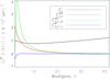Fig. 1 (Unnormalized) Integrals (Eqs. (31)–(33)) computed from a modified version of CAMB Lewis et al. (2000). The anisotropic integrals decay toward zero after only a few multipoles. These integrals are all used in constructing the signal covariance matrix. An anisotropic scalar spectral index of nde = 1.0 is used in this plot, and we have not normalized them. The amplitude ϖ0 has been set to unity.

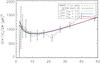Fig. 2 (Binned) Modified spectra from Eq. (35) plotted as function of dark energy spectral index. Amplitude ϖ0 = 0.9 is used in all instances. Dark energy spectral index values of nde = 0,1,2 are used in this plot. The modified spectra are plotted against the binned WMAP 7-yr data (black stapled line) and the best fit ΛCDM spectrum (black solid line). Error bars indicate 1σ cosmic variance + measurement uncertainty and have been obtained from the diagonal of the Fisher matrix supplied by the WMAP team.

We now express the integrals in Eqs. (17)–(19) in terms of power spectra C_ℓ, ${\mathit{C}}_{\mathit{\ell }{\mathit{\ell }}^{\mathrm{\prime }}}^{\mathit{A}}$, ${\mathit{C}}_{\mathit{\ell }{\mathit{\ell }}^{\mathrm{\prime }}}^{\mathit{AA}}$ as $\begin{array}{ccc}& & {\mathit{C}}_{\mathit{\ell }}\mathrm{=}\frac{\mathrm{2}}{\mathit{\pi }}{\mathit{I}}_{\mathit{\ell \ell }}\\ & & {\mathit{C}}_{\mathit{\ell }{\mathit{\ell }}^{\mathrm{\prime }}}^{\mathit{A}}\mathrm{=}\frac{\mathrm{2}}{\mathit{\pi }}{\mathit{I}}_{\mathit{\ell }{\mathit{\ell }}^{\mathrm{\prime }}}^{\mathit{A}}\\ & & {\mathit{C}}_{\mathit{\ell }{\mathit{\ell }}^{\mathrm{\prime }}}^{\mathit{AA}}\mathrm{=}\frac{\mathrm{2}}{\mathit{\pi }}{\mathit{I}}_{\mathit{\ell }{\mathit{\ell }}^{\mathrm{\prime }}}^{\mathit{AA}}\mathit{.}\end{array}$From Eqs. (17)–(19) we see that ${\mathit{C}}_{\mathit{\ell }{\mathit{\ell }}^{\mathrm{\prime }}}^{\mathit{A}}$ and ${\mathit{C}}_{\mathit{\ell }{\mathit{\ell }}^{\mathrm{\prime }}}^{\mathit{AA}}$ only give contributions for ℓ′ = ℓ ± 1 and ℓ′ = ℓ ± 2. In Fig. 1 we have calculated (using a modified version of CAMB) and plotted these integrals (because of symmetry the ℓ′ = ℓ + 1 and ℓ′ = ℓ + 2 terms are equal to the ℓ′ = ℓ − 1 and ℓ′ = ℓ − 2 terms plotted) and compared them to the isotropic power spectrum. From this figure we clearly see that the anisotropic contribution from the dark energy component becomes negligible except on the largest scales where the anisotropic contribution even exceeds the isotropic. The most prominent modification stems from the anisotropic integral ${\mathit{C}}_{\mathit{\ell \ell }\mathrm{-}\mathrm{2}}^{\mathit{AA}}$ contributing to the off-diagonal elements of the signal covariance matrix. This quadrupole modulation completely dominates the corresponding dipole modulation represented by ${\mathit{C}}_{\mathit{\ell \ell }\mathrm{-}\mathrm{1}}^{\mathit{A}}$. This is observed for all n_de values. Owing to the short range of the anisotropic integrals we altered the pivot scale in CAMB from k₀ = 0.05 Mpc^-1 to k₀ = 2 × 10^-3 Mpc^-1. In this way, we ensure that the spectral index enters correctly to tilt these integrals.

4.3. Transformation of variables

We have noticed from simulations that there was a significant degeneracy between the anisotropic spectral index n_de and the amplitude ϖ₀ because they both regulate the magnitude of the non-diagonal signal matrix elements. To ease the estimation procedure we introduce a new variable ${\mathit{\varpi }}_{\mathrm{0}}^{\mathit{a}}$ instead of ϖ₀. The “new” variable is defined as ${\mathit{\varpi }}_{\mathrm{0}}^{\mathit{a}}\mathrm{=}{\mathit{\varpi }}_{\mathrm{0}}\mathit{/}\sqrt{\mathit{a}}$ where we define a through $\mathit{a}\mathrm{=}\mathit{A}\mathrm{\left(}{\mathit{I}}_{\mathit{\ell \ell }\mathrm{-}\mathrm{2}}^{\mathrm{AA}}\mathrm{\right(}\mathrm{1.0}\mathrm{\left)}\mathrm{\right)}\mathit{/}\mathit{A}\mathrm{\left(}{\mathit{I}}_{\mathit{\ell \ell }\mathrm{-}\mathrm{2}}^{\mathrm{AA}}\mathrm{\right(}{\mathit{n}}_{\mathrm{de}}\mathrm{\left)}\mathrm{\right)}$. Here $\mathit{A}\mathrm{\left(}{\mathit{I}}_{\mathit{\ell }{\mathit{\ell }}^{\mathrm{\prime }}}^{\mathrm{X}}\mathrm{\right(}{\mathit{n}}_{\mathrm{de}}\mathrm{\left)}\mathrm{\right)}$ is the area under the anisotropic integral ${\mathit{I}}_{\mathit{\ell }{\mathit{\ell }}^{\mathrm{\prime }}}^{\mathrm{X}}\mathrm{\left(}{\mathit{n}}_{\mathrm{de}}\mathrm{\right)}$, where X = { A,AA } and n_de is the dark energy spectral index. The parameters n_de and ${\mathit{\varpi }}_{\mathrm{0}}^{\mathit{a}}$ are not degenerate and can thus more easily be estimated for. In the end, we convert to the physical parameter ϖ₀, and all results are quoted in terms of this parameter.

4.4. Modification of spectrum

The angular power spectrum C_ℓ will receive a contribution from the anisotropy that could have an observable impact at the largest scales of the universe. This can be seen from Eqs. (17)–(19) and the form of the ξ_{ℓm;ℓ′m′} elements (see Ackerman et al. 2007, for details). One must therefore be careful when performing the full analysis, making sure that any choice for ϖ₀ does not significantly drive the power spectrum away from the WMAP best fit spectrum, but mainly contributes to the anisotropic contribution to the correlations between a_ℓms.

To quantify these statements, we calculate the net extra power from the anisotropic contribution. It is given by the diagonal part of the anisotropy, which can be written as 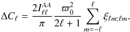$\mathrm{\Delta }{\mathit{C}}_{\mathit{\ell }}\mathrm{=}\frac{\mathrm{2}{\mathit{I}}_{\mathit{\ell \ell }}^{\mathit{AA}}}{\mathit{\pi }}\frac{{\mathit{\varpi }}_{\mathrm{0}}^{\mathrm{2}}}{\mathrm{2}\mathit{\ell }\mathrm{+}\mathrm{1}}\sum _{\mathit{m}\mathrm{=}\mathrm{-}\mathit{\ell }}^{\mathit{\ell }}{\mathit{\xi }}_{\mathit{\ell m}\mathrm{;}\mathit{\ell m}}\mathit{.}$(34)Using the explicit form of ξ_ℓm;ℓm to perform the summation, we find the modified power spectrum (see the Appendix for details): ${\mathit{C}}_{\mathit{\ell }}^{\mathrm{mod}}\mathrm{=}{\mathit{C}}_{\mathit{\ell }}\mathrm{+}\frac{\mathrm{2}}{\mathrm{3}\mathit{\pi }}{\mathit{\varpi }}_{\mathrm{0}}^{\mathrm{2}}{\mathit{I}}_{\mathit{\ell \ell }}^{\mathrm{AA}}\mathrm{\left(}{\mathit{n}}_{\mathrm{de}}\mathrm{\right)}\mathrm{\equiv }{\mathit{C}}_{\mathit{\ell }}\mathrm{+}\frac{{\mathit{\varpi }}_{\mathrm{0}}^{\mathrm{2}}}{\mathrm{3}}{\mathit{C}}_{\mathit{\ell }}^{\mathrm{AA}}\mathit{.}$(35)The extra contribution to the power spectrum from the anisotropic sources depends on the amplitude parameter ϖ₀ (degree of isotropy breaking) and the dark energy spectral index (parameterization of the fluid scale dependence), which we have included explicitly as an argument in ${\mathit{I}}_{\mathit{\ell \ell }}^{\mathrm{AA}}$.

We see from Eq. (35) that there is a limit to what values the amplitude ϖ₀ may take in order to obtain a power spectrum that is consistent with the WMAP7 best fit. This is, however, only true when we assume that the other cosmological parameters have the WMAP best fit values. Clearly the new parameters that we have introduced allow for the other parameters to vary, and one should in principle re-estimate the other cosmological parameters together with ϖ₀ and n_de. To save computational time, we chose to avoid a full re-estimation of the cosmological parameters. Instead we run the analysis in two different manners:

• 1.

  We fix the cosmological parameters to the WMAP best fitparameters. In principle one could have used only thehigh-ℓ spectrum, which is not influenced by the anisotropic model to fix the parameters, but the contribution from the lowest TT multipoles ℓ< 30 to the cosmological parameters is insignificant due to the large cosmic variance. We confirmed this using CosmoMC (Lewis & Bridle 2002) with and without the lowest multipoles.. In this case only the anisotropic parameters vary. The likelihood maximization ensures that the low-ℓ spectrum does not fluctuate far away from the best fit spectrum.

• 2.

  To test the anisotropic model without running a full cosmological parameter estimation one may renormalize the covariance matrix for a given set of parameters (ϖ₀, n_de) in such a way that the power spectrum is kept constant in the best fit WMAP model. In this case the signal covariance becomes ${\mathit{S}}_{\mathit{\ell m}\mathrm{;}{\mathit{\ell }}^{\mathrm{\prime }}{\mathit{m}}^{\mathrm{\prime }}}^{\mathrm{Norm}}\mathrm{=}\left(\frac{{\mathit{S}}_{\mathit{\ell m}\mathrm{;}{\mathit{\ell }}^{\mathrm{\prime }}{\mathit{m}}^{\mathrm{\prime }}}}{\sqrt{{\mathit{S}}_{\mathit{\ell m}\mathrm{;}\mathit{\ell m}}{\mathit{S}}_{{\mathit{\ell }}^{\mathrm{\prime }}{\mathit{m}}^{\mathrm{\prime }}\mathrm{;}{\mathit{\ell }}^{\mathrm{\prime }}{\mathit{m}}^{\mathrm{\prime }}}}}\right)\mathit{C}\ell$(36)where ${\mathit{S}}_{\mathit{\ell m}\mathrm{;}\mathit{\ell m}}\mathrm{=}{\mathit{C}}_{\mathit{\ell }}\mathrm{+}{\mathit{\xi }}_{\mathit{\ell m}\mathrm{;}\mathit{\ell m}}{\mathit{\varpi }}_{\mathrm{0}}^{\mathrm{2}}{\mathit{C}}_{\mathit{\ell }}^{\mathrm{AA}}$. With this normalization, the diagonal part of our signal covariance matrix will match the WMAP power spectrum regardless of amplitude and spectral index for the dark energy, while the off-diagonal components describe relative anisotropy. In addition, the renormalization in Eq. (36) breaks the degeneracy between the anisotropic set (ϖ₀,n_de) and the scalar power spectrum amplitude A_s. It is clear from our analysis results in Sect. 5 that by fixing the spectrum one allows anisotropic parameter values that may otherwise be excluded by the data. In this way we check that an anisotropic model is preferred by the data even when we let other cosmological parameters fluctuate outside of the bounds given by higher multipoles. If no significant detection of the anisotropic model is found even with this additional freedom, we will know that the more exact analysis will not give a detection.

4.5. Noise covariance

The noise in pixel space is assumed to be uncorrelated between pixels, i.e., ${{N}}_{\mathit{ij}}\mathrm{=}\mathrm{⟨}{\mathit{n}}_{\mathit{i}}{\mathit{n}}_{\mathit{j}}\mathrm{⟩}\mathrm{=}{\mathit{\sigma }}_{\mathit{i}}^{\mathrm{2}}\hspace{0.17em}{\mathit{\delta }}_{\mathit{ij}}$ where i and j are pixel indices, and σ_i is the noise root-mean-square deviation. The noise covariance matrix in pixel space is therefore diagonal. When transitioning to spherical harmonic space, the harmonic coefficients of the noise are correlated, and ${\mathit{N}}_{\mathit{\ell m}\mathrm{;}{\mathit{\ell }}^{\mathrm{\prime }}{\mathit{m}}^{\mathrm{\prime }}}\mathrm{=}\mathrm{⟨}{\mathit{n}}_{\mathit{\ell m}}{\mathit{n}}_{{\mathit{\ell }}^{\mathrm{\prime }}{\mathit{m}}^{\mathrm{\prime }}}^{\mathrm{\ast }}\mathrm{⟩}$ is therefore a dense matrix.

Expanding the noise harmonic coefficients in terms of pixel space quantities, we eventually find that the expression for the noise matrix in harmonic space becomes 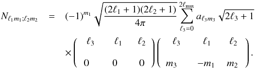$\begin{array}{ccc}{\mathit{N}}_{{\mathit{\ell }}_{\mathrm{1}}{\mathit{m}}_{\mathrm{1}}\mathrm{;}{\mathit{\ell }}_{\mathrm{2}}{\mathit{m}}_{\mathrm{2}}}& \mathrm{=}& \mathrm{(}\mathrm{-}\mathrm{1}{\mathrm{)}}^{{\mathit{m}}_{\mathrm{1}}}\sqrt{\frac{\mathrm{(}\mathrm{2}{\mathit{\ell }}_{\mathrm{1}}\mathrm{+}\mathrm{1}\mathrm{)}\mathrm{(}\mathrm{2}{\mathit{\ell }}_{\mathrm{2}}\mathrm{+}\mathrm{1}\mathrm{)}}{\mathrm{4}\mathit{\pi }}}\sum _{{\mathit{\ell }}_{\mathrm{3}}\mathrm{=}\mathrm{0}}^{\mathrm{2}{\mathit{\ell }}_{\max }}{\mathit{a}}_{{\mathit{\ell }}_{\mathrm{3}}{\mathit{m}}_{\mathrm{3}}}\sqrt{\mathrm{2}{\mathit{\ell }}_{\mathrm{3}}\mathrm{+}\mathrm{1}}\\ & & \mathrm{\times }\left(\begin{array}{c}\\ & & \\ \\ & & \end{array}\right)\left(\begin{array}{c}\\ & & \\ \\ & & \end{array}\right)\mathit{.}\end{array}$(37)The Wigner 3j symbols contain a Kroenecker delta function. It is also required that the triangle condition | ℓ₁ − ℓ₂ | ≤ ℓ₃ ≤ ℓ₁ + ℓ₂ is fulfilled. Owing to this relation the sum over ℓ₃ goes up to 2ℓ_max.

The a_ℓ3m3 coefficients stem from a spherical transform of the variance of the noise map, ${\mathit{\sigma }}_{\mathit{i}}^{\mathrm{2}}$. Equation (37) is then implemented into our code. It only needs to be computed once for each run of the code and is added to the signal covariance matrix in the step before the skycut is applied.

4.6. Correlations introduced by the mask

If we let C_{ℓm;ℓ′m′} denote the covariance matrix without mask and $\begin{array}{c}{\mathrm{˜}}_{}\\ {\mathit{C}}_{\mathit{\ell m}\mathrm{;}{\mathit{\ell }}^{\mathrm{\prime }}{\mathit{m}}^{\mathrm{\prime }}}\end{array}$ denote the corresponding matrix, including correlations from the sky cut, then the relation between them in harmonic space is 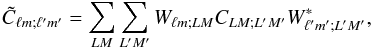$\begin{array}{c}\mathrm{˜}\\ {\mathit{C}}_{\mathit{\ell m}\mathrm{;}{\mathit{\ell }}^{\mathrm{\prime }}{\mathit{m}}^{\mathrm{\prime }}}\end{array}\mathrm{=}\sum _{\mathit{LM}}\sum _{{\mathit{L}}^{\mathrm{\prime }}{\mathit{M}}^{\mathrm{\prime }}}{\mathit{W}}_{\mathit{\ell m}\mathrm{;}\mathit{LM}}{\mathit{C}}_{\mathit{LM}\mathrm{;}{\mathit{L}}^{\mathrm{\prime }}{\mathit{M}}^{\mathrm{\prime }}}{\mathit{W}}_{{\mathit{\ell }}^{\mathrm{\prime }}{\mathit{m}}^{\mathrm{\prime }}\mathrm{;}{\mathit{L}}^{\mathrm{\prime }}{\mathit{M}}^{\mathrm{\prime }}}^{\mathrm{\ast }}\mathit{,}$(38)which can be written compactly in matrix form as $\begin{array}{c}{}_{\mathrm{˜}}\\ {C}\end{array}\mathrm{=}{WC}{{W}}^{†}$. The operation in Eq. (38) can be shown to be additive so the covariance matrix is the sum of the signal-plus-noise correlation matrices. The multipole range here is L,L′ ∈ [2,ℓ_max], and the sums over M,M′ here run over positive values. The Hermitian coupling matrix is W_{ℓm;ℓ′m′} defined by 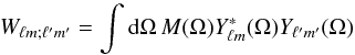${\mathit{W}}_{\mathit{\ell m}\mathrm{;}{\mathit{\ell }}^{\mathrm{\prime }}{\mathit{m}}^{\mathrm{\prime }}}\mathrm{=}\mathrm{\int }\mathrm{d\Omega }\hspace{0.17em}\mathit{M}\mathrm{\left(}\mathrm{\Omega }\mathrm{\right)}{\mathit{Y}}_{\mathit{\ell m}}^{\mathrm{\ast }}\mathrm{\left(}\mathrm{\Omega }\mathrm{\right)}{\mathit{Y}}_{{\mathit{\ell }}^{\mathrm{\prime }}{\mathit{m}}^{\mathrm{\prime }}}\mathrm{\left(}\mathrm{\Omega }\mathrm{\right)}$(39)is a function of the pixel space mask M(Ω) (where Ω = (θ,ϕ) is the angular position on the sky) and so depends on the resolution N_side. It quantifies the new couplings between modes that arise because we are now not analyzing a full sky.

Starting with the WMAP KQ85 mask at N_side = 512, we degrade our mask so that the operation of applying the mask in pixel space can be traced exactly by applying the kernel matrix W in harmonic space. This is done by first smoothing with a Gaussian beam of FWHM = 744 arcmin, and then setting M(p) = 0 (where p is a HEALPix pixel index) where M(p) < 0.80. We then band-limit the mask so that it contains multipoles in the desired range (Armendariz-Picon & Pekowsky 2008). These operations ensure that our mask does not contain small-scale structures. In the process the mask is expanded so that it now covers about 25% of the sky.

It now remains to give an expression for the coupling kernel. Equation (39) can be transformed by decomposing the mask into spherical harmonics and then performing the resulting integral over all angles to obtain again Wigner 3j symbols. This is exactly the same analytical procedure as the one that led to Eq. (37) with some minor modifications. The result in this case becomes 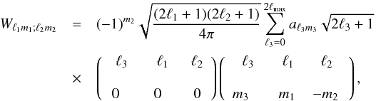$\begin{array}{ccc}{\mathit{W}}_{{\mathit{\ell }}_{\mathrm{1}}{\mathit{m}}_{\mathrm{1}}\mathrm{;}{\mathit{\ell }}_{\mathrm{2}}{\mathit{m}}_{\mathrm{2}}}& \mathrm{=}& \mathrm{(}\mathrm{-}\mathrm{1}{\mathrm{)}}^{{\mathit{m}}_{\mathrm{2}}}\sqrt{\frac{\mathrm{(}\mathrm{2}{\mathit{\ell }}_{\mathrm{1}}\mathrm{+}\mathrm{1}\mathrm{)}\mathrm{(}\mathrm{2}{\mathit{\ell }}_{\mathrm{2}}\mathrm{+}\mathrm{1}\mathrm{)}}{\mathrm{4}\mathit{\pi }}}\sum _{{\mathit{\ell }}_{\mathrm{3}}\mathrm{=}\mathrm{0}}^{\mathrm{2}{\mathit{\ell }}_{\max }}{\mathit{a}}_{{\mathit{\ell }}_{\mathrm{3}}{\mathit{m}}_{\mathrm{3}}}\sqrt{\mathrm{2}{\mathit{\ell }}_{\mathrm{3}}\mathrm{+}\mathrm{1}}\hspace{0.17em}\\ & \mathrm{\times }& \left(\begin{array}{c}\\ & & \\ \\ & & \end{array}\right)\left(\begin{array}{c}\\ & & \\ \\ & & \end{array}\right)\mathit{,}\end{array}$(40)which is almost identical to Eq. (37). As in the previous case, the internal sum covers multipoles up to 2ℓ_max, and the main difference is a change in sign of m₁,m₂. We find that the mask coupling matrix is conditioned relatively well and further manipulations are not necessary. This has been tested by simply inverting the matrix W constructed from the resulting mask, which is used in the analysis of the WMAP data.

4.7. Likelihood maximization scheme

To maximize the likelihood we use a nonlinear Newton-Rapson search algorithm² for the direction and amplitude. Finding the maximum of the likelihood is equivalent to finding the minimum of the quantity $\mathrm{-}\mathrm{2}\log \mathrm{ℒ}\mathrm{=}{{d}}^{†}{{C}}^{-1}{d}\mathrm{+}\mathrm{Tr}\log {C}\mathit{,}$(41)which has a global minimum when the likelihood function has a global maximum. The algorithm minimizes a general unconstrained function by evaluating the first and second derivatives. Thanks to the symmetry of the signal covariance matrix, ϖ₀ is constrained to be larger or equal to zero. A negative amplitude can always be replaced by a positive one and a shift in the angles (θ,ϕ): S( − ϖ₀,n_de,θ,ϕ) = S(ϖ₀,n_de,π − θ,π + ϕ). This is easily seen from the definition of the signal covariance matrix.

The gradient is computed analytically, the derivative of Eq. (41) with respect to any of the parameters in the set α is $\begin{array}{ccc}\frac{\mathit{\partial }\mathrm{(}\mathrm{-}\mathrm{2}\log \mathrm{ℒ}\mathrm{)}}{\mathit{\partial \alpha }}& \mathrm{=}& {{d}}^{†}\frac{\mathit{\partial }{{C}}^{-1}}{\mathit{\partial \alpha }}{d}\mathrm{+}\mathrm{Tr}\left(\frac{\mathit{\partial }\log {C}}{\mathit{\partial \alpha }}\right)\\ & \mathrm{=}& \end{array}$(42)To find the derivative of C^-1 we differentiated the identity matrix I = CC^-1 and solved for the derivative of the inverse covariance matrix in terms of the derivative of the matrix itself. The analytic derivative of C is computed from Eq. (12). The second derivatives are estimated from the gradient using a secant method. Depending on our initial parameter guesses and our convergence criteria, the minimizer may or may not converge in general to a global minimum. In our case, false convergence is rarely a problem since the likelihood surface is well behaved, and in rare cases, where local minima are found, they have small amplitudes compared to the global one.

For the spectral index n_de we run a grid calculation. In each grid point, we apply the above maximization procedure and find the value of the maximum likelihood for the given value of n_de. In the end we search the grid to find the full global maximum in the four-parameter space.

5. Application to WMAP-data

We now discuss the results obtained with and without normalization of our signal covariance matrix (see Sect. 4.4). We analyze the V-band (61 GHz) data map, which is believed to be one of the cleanest bands in terms of foreground residuals, and recommended for cosmological analysis by the WMAP team. To this map we apply the modified WMAP KQ85 galactic skycut, removing 25% of the sky. Since we are only analyzing the largest scales no special care is taken with regards to point-source masking. We take the V-band noise RMS pattern and the corresponding beam properties into account. We analyze these maps up to a maximum multipole moment ℓ_max = 20. The kernel matrices W that emulate the effect of a skycut in harmonic space includes multipoles up to ℓ_max = 40. Now that we have our data map, we are ready to start the analysis.

5.1. Unnormalized covariance matrix

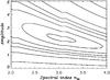Fig. 3 Two-dimensional plot of the raw likelihood (posterior distribution) as a function of dark energy spectral index nde and the transformed amplitude ${\mathit{\varpi }}_{\mathrm{0}}^{\mathit{a}}$, using WMAP 7-yr data. The spherical angles have been fixed to their WMAP best fit values at ℓmax = 20 to enable a projection. The posterior mode value is located at nde = 3.1. The (transformed) amplitude found in this plot is higher than the value for the true anisotropic amplitude noted in Table 1 due to a bias introduced by application of the mask and a linear transformation.

Performing a grid-calculation with a spectral index range of − 5 ≤ n_de ≤ 5 with a stepsize of Δn_de = 0.1, where for each value of n_de, we do a three-dimensional search for the peak of the likelihood function using our likelihood maximization scheme described in Sect. 4.7. We find that the likelihood values for negative spectral index values are very insignificant. As we approach n_de = 0, the likelihood starts peaking slowly until we find a peak at n_de = 3.1. The best fit direction remains practically constant as we move through the grid (the change is completely negligible compared to the uncertainty) indicating that the correlation between the two sets (θ,ϕ) and (n_de,ϖ₀) is weak.

We find Fisher matrix error bars calculating the Fisher matrix using ${\mathit{F}}_{\mathit{\alpha \beta }}\mathrm{=}\frac{\mathrm{1}}{\mathrm{2}}\mathrm{Tr}\left(\frac{\mathrm{d}\mathit{C}}{\mathrm{d}{\mathit{\lambda }}_{\mathit{\alpha }}}{\mathit{C}}^{-1}\frac{\mathrm{d}\mathit{C}}{\mathrm{d}{\mathit{\lambda }}_{\mathit{\beta }}}{\mathit{C}}^{-1}\right)\mathit{,}$(43)where the derivatives of the covariance matrix are found analytically for the direction and amplitude and numerically for the spectral index. Since the amplitude and spectral index are weakly correlated, the off-diagonal elements are taken into account in the matrix. The results are shown in Table 1. As expected, in order for the model to be consistent with the power spectrum, we find ϖ₀ consistent with zero within the 1σ error. In Fig. 3 we show the likelihood surface close to the peak. The amplitude in this plot is the transformed amplitude ${\mathit{\varpi }}_{\mathrm{0}}^{\mathit{a}}$ (see Sect. 4.3), and the amplitude at the maximum of the likelihood is biased with respect to the best fit amplitude. This bias results from the complicated form of the likelihood introduced by the mask. The bias is corrected for in the following manner: given the parameters found from the peak of the likelihood, we generate 100 anisotropic realizations. For each realization we estimate the anisotropic parameters, and in the end compute the average bias in ${\mathit{\varpi }}_{\mathrm{0}}^{\mathit{a}}$. Next we subtract the bias from the input value and repeat the procedure until our average computed amplitude matches the value found in the WMAP data. When the bias has been subtracted, we are left with “the true” estimate of the transformed amplitude ${\mathit{\varpi }}_{\mathrm{0}}^{\mathit{a}}$. The original amplitude is then obtained using ${\mathit{\varpi }}_{\mathrm{0}}\mathrm{=}\sqrt{\mathit{a}}{\mathit{\varpi }}_{\mathrm{0}}^{\mathit{a}}$. In the unnormalized case we find a final amplitude value ϖ₀ = 0.51.

The best fit direction is somewhat close to the galactic center. To check that this is not caused by the shape of the mask, we estimated the direction on 1000 simulated isotropic maps and found that there is no bias toward the galactic center. The estimated directions are shown in Fig. 4.

The error in the amplitude has also been estimated using 1000 Monte Carlo simulations. We find that the error from simulations agrees well with the error found using the Fisher matrix. In Fig. 5 we show the best fit direction with error bars.

Fig. 4 Distribution of (θ,ϕ) values on the sphere from Gaussian (ϖ0 = 0 input) simulations. The positions found in the simulations are randomly distributed on the sphere and not aligned along some particular axis, in clear agreement with a random Gaussian distribution.

Fig. 5 Map indicating the 1σ uncertainty in the preferred direction of the axis. The background is the V-band (61 GHz) WMAP 7-yr data map with the KQ85 mask. The two axes plotted are the directions given in Table 1 for the unnormalized and the normalized cases.

An isotropic universe is clearly preferred by the data when using this model.

5.2. Normalized covariance matrix

The model with an unnormalized matrix (see Eq. (12)) giving the modified power spectrum in Eq. (35) is clearly not preferred by the WMAP 7-yr data. However, if we allow other cosmological parameters to vary we may be able to find a better fit as explained above. We therefore repeated the procedure using the normalization in Eq. (36), which means fixing the diagonal part of the covariance matrix to the best fit C_ℓ regardless of amplitude and spectral index.

The lower line in Table 1 shows the results for the anisotropic cosmological parameters from the exploration of the likelihood space with a normalized covariance matrix. Again, a grid was set up for the spectral index in the interval − 5 ≤ n_de ≤ 5 with the same stepsize and for each value of n_de, we estimated the best fit values of (θ,ϕ,ϖ₀) and the corresponding value of the likelihood. The preferred amplitude is large in this case, but only about 2σ away from zero. The result is not very consistent with the istropic power spectrum, but a joint fit of the standard model and anisotropy parameters together could yield a lower amplitude because the diagonal contribution from the anisotropy to the covariance matrix has a low statistical weight due to the high sample variance at large scales.

6. Conclusions

In this work we tested anisotropic dark energy models with the seven-year WMAP temperature observation data. Since the completion of this analysis, the WMAP team released their nine-year data set. In addition, the Planck data has been made available. It is, however, possible to argue for the validity of our analysis with seven years of WMAP data since only the very low-ℓ data is used. WMAP seven-year data was already completely cosmic-variance-dominated at these scales, the highly reduced noise and smaller beam size of the Planck data only increased the signal-to-noise ratio at much higher multipoles. Whereas the larger frequency range of the Planck experiment in principle improves the foreground subtraction at low multipoles, it has been shown in practice that the differences between Planck and WMAP at these very low multipoles ℓ< 20 are much less than the cosmic variance (Planck Collaboration XV 2014). The error bars presented in this paper are therefore cosmic-variance-dominated and an analysis of the Planck data would not add new information.

If dark energy is not a perfect fluid but, for instance, a vector field, the CMB sky will be distorted anisotropically on its way to us by the ISW effect. The signal covariance matrix then becomes non-diagonal for small multipoles, but the anisotropy is negligible at ℓ ≳ 20. This can be used to constrain violations of rotational invariance in the late universe and to obtain hints on the possible imperfect nature of dark energy and the large-angle anomalous features in the CMB.

To model this phenomenon, we introduced a mismatch of the two gravitational potentials in the Newtonian gauge. The mismatch, quantified by ϖ, is proportional to a gradient along the preferred axis . We also allowed this effect to depend on the scale by introducing the spectral index n_de. Physically, such gradient could be caused by a large-scale inhomogeneity entering our horizon, spontaneous formation due to, say, coherent magnetic fields or simply to the possible imperfect nature of the dark energy field. Many possible realizations of the latter possibility were discussed in the introduction and in Sect. 3. The dominant effect on the CMB is then a quadrupole modulation (i.e., a Δℓ = 2 correlation type, see Eq. (15)), which has the same geometrical correlation structure but different time and scale dependence than in the models considered previously. Now in addition a dipole modulation, though subdominant, is predicted from the cross-term between the quadrupole modulation and the isotropic contribution (i.e., a Δℓ = 1 type correlation, see Eq. (14)).

We calculate the mode couplings introduced in the spherical harmonic coefficients of the CMB by the anisotropic model and obtain the full likelihood for the lowest multipoles where the dominant contribution to the model is expected to be found. Maximizing the likelihood when taking the instrumental parameters of the WMAP experiment into account, we are able to find optimal estimates of the anisotropic parameters. Analysis of the masked WMAP V-band, when fixing other cosmological parameters, gave a best fit amplitude ϖ₀ = 0.51 ± 0.94 and n_de = 3.1 consistent with an isotropic universe.

In comparison, tests of the isotropic version of this parameterization show that the data is then compatible with a vanishing deviation, and allows a nonzero ϖ on the order of (Daniel et al. 2010). At the level of solar system, no hints of deviations are observed, and the post-Newtonian correction is constrained to be at most (Will 2001). However, the numbers themselves cannot be directly compared, since our best fit model also features a strong scale dependence of the deviation.

Another shortcoming of our parameterization is its inability to incorporate the lack of large-angle power in the observed sky, one of the most striking anomalies present in the data. This justifies further investigation the possible origin and constraints of imperfect source terms in cosmology. In particular, a fully consistent post-Friedmannian parameterization along the lines of Ferreira & Skordis (2010) and Baker et al. (2011), when tailored to the study of directional dependence of deviations from the standard predictions of linearized cosmology, remains to be developed.

Acknowledgments

We thank Hans Kristian Eriksen for useful discussions. The work of T.K. was supported by the Academy of Finland and the Yggdrasil grant from the Norwegian Research Council. D.F.M. and F.K.H. thank the Research Council of Norway for FRINAT grant 197251/V30 and an OYI-grant respectively. D.F.M. acknowledges the support of Fundação para a Ciência e a Tecnologia (FCT), Portugal, in the form of the grant PTDC/FIS/111725/2009. D.F.M. is also partially supported by project PTDC/FIS/111725/2009 and CERN/FP/123618/2011. Maps and results have been derived using the Healpix³ software package developed by Gorski et al. (2005). The anisotropic transfer functions have been derived using a modified version of CAMB due to Lewis et al. (2000). We acknowledge the use of the LAMBDA archive (Legacy Archive for Microwave Background Data Analysis). Support for LAMBDA is provided by the NASA office for Space Science.

References

Appendix A: Anisotropic contribution to the power spectrum

The diagonal part of the covariance matrix is a sum of the power spectrum due to the isotropy and a term determined by the anisotropic parameters ϖ₀, n_de and (θ,ϕ): 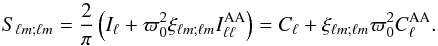${\mathit{S}}_{\mathit{\ell m}\mathrm{;}\mathit{\ell m}}\mathrm{=}\frac{\mathrm{2}}{\mathit{\pi }}\mathrm{(}{\mathit{I}}_{\mathit{\ell }}\mathrm{+}{\mathit{\varpi }}_{\mathrm{0}}^{\mathrm{2}}{\mathit{\xi }}_{\mathit{\ell m}\mathrm{;}\mathit{\ell m}}{{\mathit{I}}_{\mathit{\ell \ell }}^{\mathrm{AA}}}^{\mathrm{)}}\mathrm{=}{\mathit{C}}_{\mathit{\ell }}\mathrm{+}{\mathit{\xi }}_{\mathit{\ell m}\mathrm{;}\mathit{\ell m}}{\mathit{\varpi }}_{\mathrm{0}}^{\mathrm{2}}{\mathit{C}}_{\mathit{\ell }}^{\mathrm{AA}}\mathit{.}$(A.1)The dependence on the spectral index comes from the integral over the anisotropic transfer functions in ${\mathit{I}}_{\mathit{\ell \ell }}^{\mathrm{AA}}$. The diagonal part of the geometric factor is (Ackerman et al. 2007): 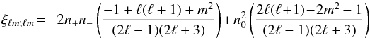${\mathit{\xi }}_{\mathit{\ell m}\mathrm{;}\mathit{\ell m}}\mathrm{=}\mathrm{-}\mathrm{2}{\mathit{n}}_{\mathrm{+}}{\mathit{n}}_{\mathrm{-}}\left(\frac{\mathrm{-}\mathrm{1}\mathrm{+}\mathit{\ell }\mathrm{(}\mathit{\ell }\mathrm{+}\mathrm{1}\mathrm{)}\mathrm{+}{\mathit{m}}^{\mathrm{2}}}{\mathrm{(}\mathrm{2}\mathit{\ell }\mathrm{-}\mathrm{1}\mathrm{)}\mathrm{(}\mathrm{2}\mathit{\ell }\mathrm{+}\mathrm{3}\mathrm{)}}\right)\mathrm{+}{\mathit{n}}_{\mathrm{0}}^{\mathrm{2}}\left(\frac{\mathrm{2}\mathit{\ell }\mathrm{(}\mathit{\ell }\mathrm{+}\mathrm{1}\mathrm{)}\mathrm{-}\mathrm{2}{\mathit{m}}^{\mathrm{2}}\mathrm{-}\mathrm{1}}{\mathrm{(}\mathrm{2}\mathit{\ell }\mathrm{-}\mathrm{1}\mathrm{)}\mathrm{(}\mathrm{2}\mathit{\ell }\mathrm{+}\mathrm{3}\mathrm{)}}\right)$(A.2)where the spherical components n₊,n₋,n₀ containing the angular dependence have been defined in Eq. (10). Using a well-known result from Mathematics: $\sum _{\mathit{m}\mathrm{=}\mathrm{1}}^{\mathit{\ell }}{\mathit{m}}^{\mathrm{2}}\mathrm{=}\frac{\mathit{\ell }\mathrm{(}\mathit{\ell }\mathrm{+}\mathrm{1}\mathrm{)}\mathrm{(}\mathrm{2}\mathit{\ell }\mathrm{+}\mathrm{1}\mathrm{)}}{\mathrm{6}}$(A.3)we find that the average of the geometric factor is free from angular dependence and simplifies nicely to $\sum _{\mathit{m}\mathrm{=}\mathrm{-}\mathit{\ell }}^{\mathit{\ell }}{\mathit{\xi }}_{\mathit{\ell m}\mathrm{;}\mathit{\ell m}}\mathrm{=}\frac{\mathrm{2}\mathit{\ell }\mathrm{+}\mathrm{1}}{\mathrm{3}}\mathrm{·}$(A.4)With this result one finds that the theoretical prediction for the modified power spectrum due to the anisotropic component becomes 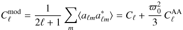${\mathit{C}}_{\mathit{\ell }}^{\mathrm{mod}}\mathrm{=}\frac{\mathrm{1}}{\mathrm{2}\mathit{\ell }\mathrm{+}\mathrm{1}}\sum _{\mathit{m}}\mathrm{⟨}{\mathit{a}}_{\mathit{\ell m}}{\mathit{a}}_{\mathit{\ell m}}^{\mathrm{\ast }}\mathrm{⟩}\mathrm{=}{\mathit{C}}_{\mathit{\ell }}\mathrm{+}\frac{{\mathit{\varpi }}_{\mathrm{0}}^{\mathrm{2}}}{\mathrm{3}}\hspace{0.17em}{\mathit{C}}_{\mathit{\ell }}^{\mathrm{AA}}$(A.5)which is the modified power spectrum ${\mathit{C}}_{\mathit{\ell }}^{\mathrm{mod}}$ quoted in Eq. (35).

All Tables

All Figures

Fig. 1 (Unnormalized) Integrals (Eqs. (31)–(33)) computed from a modified version of CAMB Lewis et al. (2000). The anisotropic integrals decay toward zero after only a few multipoles. These integrals are all used in constructing the signal covariance matrix. An anisotropic scalar spectral index of nde = 1.0 is used in this plot, and we have not normalized them. The amplitude ϖ0 has been set to unity.

In the text

Fig. 2 (Binned) Modified spectra from Eq. (35) plotted as function of dark energy spectral index. Amplitude ϖ0 = 0.9 is used in all instances. Dark energy spectral index values of nde = 0,1,2 are used in this plot. The modified spectra are plotted against the binned WMAP 7-yr data (black stapled line) and the best fit ΛCDM spectrum (black solid line). Error bars indicate 1σ cosmic variance + measurement uncertainty and have been obtained from the diagonal of the Fisher matrix supplied by the WMAP team.

In the text

Fig. 3 Two-dimensional plot of the raw likelihood (posterior distribution) as a function of dark energy spectral index nde and the transformed amplitude ${\mathit{\varpi }}_{\mathrm{0}}^{\mathit{a}}$, using WMAP 7-yr data. The spherical angles have been fixed to their WMAP best fit values at ℓmax = 20 to enable a projection. The posterior mode value is located at nde = 3.1. The (transformed) amplitude found in this plot is higher than the value for the true anisotropic amplitude noted in Table 1 due to a bias introduced by application of the mask and a linear transformation.

In the text

	Fig. 4 Distribution of (θ,ϕ) values on the sphere from Gaussian (ϖ0 = 0 input) simulations. The positions found in the simulations are randomly distributed on the sphere and not aligned along some particular axis, in clear agreement with a random Gaussian distribution.
In the text

	Fig. 5 Map indicating the 1σ uncertainty in the preferred direction of the axis. The background is the V-band (61 GHz) WMAP 7-yr data map with the KQ85 mask. The two axes plotted are the directions given in Table 1 for the unnormalized and the normalized cases.
In the text

References

- Abramo, L. R., & Pereira, T. S. 2010, Adv. Astron., id. 378203 [Google Scholar]
- Ackerman, L., Carroll, S. M., & Wise, M. B. 2007, Phys. Rev. D, 75, 083502 [NASA ADS] [CrossRef] [Google Scholar]
- Adamek, J., Campo, D., & Niemeyer, J. C. 2010, Phys. Rev. D, 82, 086006 [NASA ADS] [CrossRef] [Google Scholar]
- Afshordi, N., Geshnizjani, G., & Khoury, J. 2009, JCAP, 0908, 030 [NASA ADS] [CrossRef] [Google Scholar]
- Akarsu, O., & Kilinc, C. B. 2010, Gen. Rel. Grav., 42, 763 [Google Scholar]
- Aluri, P. K., & Jain, P. 2012, MNRAS, 419, 3378 [NASA ADS] [CrossRef] [Google Scholar]
- Amendola, L., Appleby, S., Bacon, D., et al. 2013, Liv. Rev. Relat., 16, 6 [Google Scholar]
- Appleby, S., Battye, R., & Moss, A. 2010, Phys. Rev. D, 81, 081301 [NASA ADS] [CrossRef] [Google Scholar]
- Armendariz-Picon, C. 2004, JCAP, 0407, 007 [NASA ADS] [CrossRef] [Google Scholar]
- Armendariz-Picon, C., & Pekowsky, L. 2008 [arXiv:0807.2687] [Google Scholar]
- Axelsson, M., Fantaye, Y., Hansen, F. K., et al. 2013, ApJ, 773, L3 [NASA ADS] [CrossRef] [Google Scholar]
- Baker, T., Ferreira, P. G., Skordis, C., & Zuntz, J. 2011, Phys. Rev. D, 84, 124018 [NASA ADS] [CrossRef] [Google Scholar]
- Bartolo, N., Dimastrogiovanni, E., Matarrese, S., & Riotto, A. 2009a, JCAP, 10, 15 [NASA ADS] [CrossRef] [Google Scholar]
- Bartolo, N., Dimastrogiovanni, E., Matarrese, S., & Riotto, A. 2009b, JCAP, 11, 28 [NASA ADS] [CrossRef] [Google Scholar]
- Bartolo, N., Dimastrogiovanni, E., Liguori, M., Matarrese, S., & Riotto, A. 2012, J. Cosmology Astropart. Phys., 1, 29 [NASA ADS] [CrossRef] [Google Scholar]
- Battye, R., & Moss, A. 2009, Phys. Rev. D, 80, 023531 [NASA ADS] [CrossRef] [Google Scholar]
- Beltran Jimenez, J., & Maroto, A. L. 2010, Phys. Lett. B, 686, 175 [NASA ADS] [CrossRef] [Google Scholar]
- Bennett, C. L., Halpern, M., Hinshaw, G., et al. 2003, ApJS, 148, 1 [NASA ADS] [CrossRef] [Google Scholar]
- Bennett, C. L., Hill, R. S., Hinshaw, G., et al. 2011, ApJS, 192, 17 [NASA ADS] [CrossRef] [Google Scholar]
- Bennett, C. L., Larson, D., Weiland, J. L., et al. 2013, ApJS, 208, 20 [Google Scholar]
- Boehmer, C. G., & Mota, D. F. 2008, Phys. Lett. B, 663, 168 [NASA ADS] [CrossRef] [Google Scholar]
- Caldwell, R., Cooray, A., & Melchiorri, A. 2007, Phys. Rev. D, 76, 023507 [NASA ADS] [CrossRef] [Google Scholar]
- Campanelli, L. 2009, Phys. Rev. D, 80, 063006 [NASA ADS] [CrossRef] [Google Scholar]
- Cooke, R., & Lynden-Bell, D. 2010, MNRAS, 401, 1409 [NASA ADS] [CrossRef] [Google Scholar]
- Cooray, A., Holz, D. E., & Caldwell, R. 2010, J. Cosmology Astropart. Phys., 11, 15 [Google Scholar]
- Copi, C. J., Huterer, D., Schwarz, D. J., & Starkman, G. D. 2010, Adv. Astron., 847541 [Google Scholar]
- Daniel, S. F., Caldwell, R. R., Cooray, A., & Melchiorri, A. 2008, Phys. Rev. D, 77, 103513 [NASA ADS] [CrossRef] [Google Scholar]
- Daniel, S. F., Caldwell, R. R., Cooray, A., Serra, P., & Melchiorri, A. 2009, Phys. Rev. D, 80, 023532 [NASA ADS] [CrossRef] [Google Scholar]
- Daniel, S. F., Linder, E. V., Smith, T. L., et al. 2010, Phys. Rev. D, 81, 123508 [NASA ADS] [CrossRef] [Google Scholar]
- Dimastrogiovanni, E., Fischler, W., & Paban, S. 2008, JHEP, 07, 045 [NASA ADS] [CrossRef] [Google Scholar]
- Dimastrogiovanni, E., Bartolo, N., Matarrese, S., & Riotto, A. 2010, Adv. Astron., id. 752670 [Google Scholar]
- Dimopoulos, K., Karciauskas, M., Lyth, D. H., & Rodríguez, Y. 2009, JCAP, 5, 13 [NASA ADS] [CrossRef] [Google Scholar]
- Dimopoulos, K., Karciauskas, M., & Wagstaff, J. M. 2010, Phys. Rev. D, 81, 023522 [NASA ADS] [CrossRef] [Google Scholar]
- Dimopoulos, K., Wills, D., & Zavala, I. 2013, Nucl. Phys. B, 868, 120 [NASA ADS] [CrossRef] [Google Scholar]
- Dvali, G. R., Gabadadze, G., & Porrati, M. 2000, Phys. Lett. B, 485, 208 [NASA ADS] [CrossRef] [MathSciNet] [Google Scholar]
- Erickcek, A. L., Kamionkowski, M., & Carroll, S. M. 2008, Phys. Rev. D, 78, 123520 [NASA ADS] [CrossRef] [Google Scholar]
- Eriksen, H. K., Hansen, F. K., Banday, A. J., Gorski, K. M., & Lilje, P. B. 2004, ApJ, 605, 14 [NASA ADS] [CrossRef] [Google Scholar]
- Ferreira, P. G., & Skordis, C. 2010, Phys. Rev. D, 81, 104020 [NASA ADS] [CrossRef] [Google Scholar]
- Germani, C., & Kehagias, A. 2009, JCAP, 0903, 028 [NASA ADS] [CrossRef] [Google Scholar]
- Gies, H., Mota, D. F., & Shaw, D. J. 2008, Phys. Rev. D, 77, 025016 [NASA ADS] [CrossRef] [Google Scholar]
- Golovnev, A., Mukhanov, V., & Vanchurin, V. 2008, JCAP, 0806, 009 [NASA ADS] [CrossRef] [Google Scholar]
- Gordon, C., Hu, W., Huterer, D., & Crawford, T. M. 2005, Phys. Rev. D, 72, 103002 [NASA ADS] [CrossRef] [Google Scholar]
- Gorski, K. M., et al. 2005, ApJ, 622, 759 [NASA ADS] [CrossRef] [Google Scholar]
- Graham, P. W., Harnik, R., & Rajendran, S. 2010, Phys. Rev. D, 82, 063524 [NASA ADS] [CrossRef] [Google Scholar]
- Groeneboom, N. E., & Eriksen, H. K. 2009, ApJ, 690, 1807 [NASA ADS] [CrossRef] [Google Scholar]
- Groeneboom, N. E., Axelsson, M., Mota, D. F., & Koivisto, T. 2010 [arXiv:1011.5353] [Google Scholar]
- Gumrukcuoglu, A. E., Contaldi, C. R., & Peloso, M. 2006, unpublished [arXiv:0608405] [Google Scholar]
- Gumrukcuoglu, A. E., Contaldi, C. R., & Peloso, M. 2007, JCAP, 0711, 005 [CrossRef] [Google Scholar]
- Hansen, F. K., Banday, A. J., Gorski, K. M., Eriksen, H. K., & Lilje, P. B. 2008, 0812.3795 [Google Scholar]
- Hinshaw, G., Nolta, M. R., Bennett, C. L., et al. 2007, ApJS, 170, 288 [NASA ADS] [CrossRef] [Google Scholar]
- Hoftuft, J., Eriksen, H. K., Banday, A. J., et al. 2009, ApJ, 699, 985 [NASA ADS] [CrossRef] [Google Scholar]
- Hu, W., & Sawicki, I. 2007, Phys. Rev. D, 76, 104043 [NASA ADS] [CrossRef] [Google Scholar]
- Jimenez, J. B., & Maroto, A. L. 2008, Phys. Rev. D, 78, 063005 [NASA ADS] [CrossRef] [Google Scholar]
- Jimenez, J. B., & Maroto, A. L. 2009, JCAP, 0903, 016 [CrossRef] [Google Scholar]
- Jimenez, J. B., Koivisto, T. S., Maroto, A. L., & Mota, D. F. 2009, JCAP, 0910, 029 [CrossRef] [Google Scholar]
- Kiselev, V. V. 2004, Class. Quant. Grav., 21, 3323 [NASA ADS] [CrossRef] [Google Scholar]
- Koivisto, T., & Mota, D. F. 2006, Phys. Rev. D, 73, 083502 [NASA ADS] [CrossRef] [MathSciNet] [Google Scholar]
- Koivisto, T., & Mota, D. F. 2008a, JCAP, 0806, 018 [NASA ADS] [CrossRef] [Google Scholar]
- Koivisto, T. S., & Mota, D. F. 2008b, JCAP, 0808, 021 [NASA ADS] [CrossRef] [Google Scholar]
- Koivisto, T. S., & Mota, D. F. 2011, JHEP, 1102, 061 [NASA ADS] [CrossRef] [Google Scholar]
- Koivisto, T. S., & Nunes, N. J. 2009, Phys. Rev. D, 80, 103509 [NASA ADS] [CrossRef] [Google Scholar]
- Koivisto, T. S., Mota, D. F., & Pitrou, C. 2009, J. High Energy Physics, 9, 92 [NASA ADS] [CrossRef] [Google Scholar]
- Koivisto, T. S., Mota, D. F., Quartin, M., & Zlosnik, T. G. 2011, Phys. Rev. D, 83, 023509 [NASA ADS] [CrossRef] [Google Scholar]
- Land, K., & Magueijo, J. 2005, Phys. Rev. Lett., 95, 071301 [NASA ADS] [CrossRef] [PubMed] [Google Scholar]
- Land, K., & Magueijo, J. 2007, MNRAS, 378, 153 [NASA ADS] [CrossRef] [Google Scholar]
- Lewis, A., & Bridle, S. 2002, Phys. Rev. D, 66, 103511 [NASA ADS] [CrossRef] [Google Scholar]
- Lewis, A., Challinor, A., & Lasenby, A. 2000, ApJ, 538, 473 [NASA ADS] [CrossRef] [Google Scholar]
- Li, B., Fonseca Mota, D., & Barrow, J. D. 2008, Phys. Rev. D, 77, 024032 [NASA ADS] [CrossRef] [MathSciNet] [Google Scholar]
- Libanov, M., Rubakov, V., Papantonopoulos, E., Sami, M., & Tsujikawa, S. 2007, JCAP, 0708, 010 [NASA ADS] [CrossRef] [Google Scholar]
- Manera, M., & Mota, D. 2006, MNRAS, 371, 1373 [NASA ADS] [CrossRef] [Google Scholar]
- Mota, D. F., Kristiansen, J. R., Koivisto, T., & Groeneboom, N. E. 2007, MNRAS, 382, 793 [NASA ADS] [CrossRef] [Google Scholar]
- Pereira, T. S., Pitrou, C., & Uzan, J.-P. 2007, JCAP, 0709, 006 [NASA ADS] [CrossRef] [Google Scholar]
- Planck Collaboration I. 2014, A&A, in press [arXiv:1303.5062] [Google Scholar]
- Planck Collaboration XV. 2014, A&A, in press [arXiv:1303.5075] [Google Scholar]
- Planck Collaboration XXIII. 2014, A&A, in press DOI: 10.1051/0004-6361/201321534 [Google Scholar]
- Prunet, S., Uzan, J.-P., Bernardeau, F., & Brunier, T. 2005, Phys. Rev. D, 71, 083508 [NASA ADS] [CrossRef] [Google Scholar]
- Rakic, A., & Schwarz, D. J. 2007, Phys. Rev. D, 75, 103002 [NASA ADS] [CrossRef] [Google Scholar]
- Rodrigues, D. C. 2008, Phys. Rev. D, 77, 023534 [NASA ADS] [CrossRef] [Google Scholar]
- Rubakov, V. A. 2006, Theor. Math. Phys., 149, 1651 [CrossRef] [Google Scholar]
- Skordis, C. 2009, Phys. Rev. D, 79, 123527 [NASA ADS] [CrossRef] [Google Scholar]
- Tangen, K. 2009, Phys. Rev. D, accepted [arXiv:0910.4164] [Google Scholar]
- Watanabe, M., Kanno, S., & Soda, J. 2010, Prog. Theoret. Phys., 123, 1041 [Google Scholar]
- Watanabe, M.-A., Kanno, S., & Soda, J. 2009, Phys. Rev. Lett., 102, 191302 [NASA ADS] [CrossRef] [PubMed] [Google Scholar]
- Watanabe, M.-A., Kanno, S., & Soda, J. 2011, MNRAS, 412, L83 [Google Scholar]
- Will, C. M. 2001, Liv. Rev. Rel., 4, 4 [Google Scholar]
- Yokoyama, S., & Soda, J. 2008, JCAP, 8, 5 [NASA ADS] [CrossRef] [Google Scholar]
- Zlosnik, T. 2011, unpublished [arXiv:1107.0389] [Google Scholar]
- Zuntz, J., Zlosnik, T. G., Bourliot, F., Ferreira, P. G., & Starkman, G. D. 2010, Phys. Rev. D, 81, 104015 [NASA ADS] [CrossRef] [Google Scholar]