| Issue |
A&A
Volume 563, March 2014
|
|
|---|---|---|
| Article Number | A23 | |
| Number of page(s) | 8 | |
| Section | Stellar structure and evolution | |
| DOI | https://doi.org/10.1051/0004-6361/201323277 | |
| Published online | 27 February 2014 | |
Fundamental stellar parameters of three Kepler stars accurately constrained by lithium abundance and rotation
Department of Astronomy, Beijing Normal University, 100875 Beijing, PR China
e-mail: liukang@mail.bnu.edu.cn; bisl@bnu.edu.cn
Received: 18 December 2013
Accepted: 27 January 2014
Aims. The lithium abundances of KIC 11395018 and KIC 10920273 are not compatible with the age of these stars, which is deduced by asteroseismology. To explain this phenomenon, we investigated the possible evolutionary status and performed a seismological analysis of the three stars KIC 11395018, KIC 10273246, and KIC 10920273.
Methods. Using the Yale Rotating Stellar Evolution Code (YREC), we constructed stellar models that include diffusion and extra-mixing caused by rotation. In addition to the general observed properties, we considered two constraints, the lithium abundance log N(Li) and the rotational period Prot.
Results. A set of stellar fundamental parameters is given by our rotating model for each star. We estimate the mass and age to be 1.24 ± 0.01 M⊙ and 5.55 ± 0.20 Gyr for KIC 11395018, 1.19 ± 0.04 M⊙ and 4.36 ± 0.29 Gyr for KIC 10273246, and 1.15 ± 0.03 M⊙ and 5.68 ± 0.30 Gyr for KIC 10920273. Moreover, the lithium abundance of our rotating model of the three stars agrees well with the observation.
Conclusions. The consideration of lithium and the rotational period helped us in obtaining very precise estimates of the star.
Key words: stars: evolution / stars: rotation / stars: oscillations
© ESO, 2014
1. Introduction
Since the start of the Kepler science operations, several stars have been continuously observed at short-cadence to test and validate the time-series photometry (Gilliland et al. 2010). We studied three of these stars that have clear solar-like oscillation. Their identities in the Kepler Input Catalogue (KIC) are as follows: KIC 11395018, KIC 10273246, and KIC 10920273. They were classified as G4-5IV-V, F9IV-V, and G1-2V, with Kepler magnitudes (Kp) = 10.762, 10.903, and 11.926 mag, respectively. Because these stars have been studied in several studies, we refer to them as C1, C2, and C3 for consistency and convenience. The characteristics of these stars were summarized by Creevey et al. (2012), who provided the fundamental properties of the stars, including the radius, age, luminosity, and rotational rate, and the ranges of mass are 1.34 ± 0.11 for C1, 1.25 ± 0.10 for C2, and 1.23 ± 0.11 for C3 (see their table 9). Furthermore, 25 individual frequencies of C1 were provided by Mathur et al. (2011), 30 and 21 individual frequencies of the other stars were derived by Campante et al. (2011).
Creevey et al. (2012) showed that C1 and C3 have strong Li absorption lines, which implies a high Li content at the surface, log N(Li) = 2.6 ± 0.1 for C1 and log N(Li) = 2.4 ± 0.1 for C3. Considering the empirical Li–age relation established by Sestito et al. (2005), Creevey et al. (2012) then determined that the given Li abundances would indicate young ages (0.1−0.4 Gyr for C1 and 1−3 Gyr for C3), which are incompatible with the asteroseismic ages they determined through the pipeline modeling performed using the average asteroseismic quantities.
Currently, asteroseismology has become not only a useful method for testing theories of stellar structure and evolution, but also a powerful tool for constraining the stellar parameters. Its observational data, such as the large and small frequency separation, provide a very good measurement of the mass, radius, and age of the stars, and the large and small frequency separation are independent of the metallicity in their uncertainty range. In addition, the surface lithium abundance observed in solar-like stars was considered to be an extraordinarily sensitive diagnostic of stellar structure and evolution because lithium is easily burned at relatively low temperature (~2.5 × 10⁶ K) in the stellar interior. Consequently, the combination of accurate lithium abundance measurement and rotating model helps to provide more precise information about the stellar parameters (do Nascimento et al. 2009; Castro et al. 2011; Li et al. 2012).
In this work, we construct evolutionary models that include microscopic diffusion and mixing driven by rotation. Based on two observed constraints (Teff and L/L⊙), two additional observed limits, the lithium abundance log N (Li) and the rotational period Prot, are considered to constrain the stellar models. For the lithium abundance, we assumed that lithium depletion starts at pre-main-sequence (pre-MS) and experiences dissimilar evolution with different initial rotational rates.
In Sect. 2, we summarize the observations of the three stars. In Sect. 3, the details of the evolutionary models and seismic analysis are presented. In Sect. 4, we describe our modeling results. Finally, the discussion and conclusion are given in Sect. 5.
2. Observation
2.1. Non asteroseismic observational constraints
Observational constraint of the three stars.
The three targets C1, C2, and C3 were observed by Creevey et al. (2012) using the FIES spectrograph on the Nordic Optical Telescope (NOT) located at the Observatorio del Roque de los Muchachos in La Palma during July and August 2010. Each target was observed twice to give a total exposure time of 46, 46, and 60 min, respectively. This resulted in an signal-to-noise ratio (S/N) of ~80, 90, and 60 in the wavelength region of 6069−6076 Å. The calibration frames were taken using a Th-Ar lamp. The spectra were reduced using FIESTOOL. The reduced spectra were analyzed by several groups independently using the following methods: SOU (Sousa et al. 2007, 2008), VWA (Bruntt et al. 2010), ROTFIT (Frasca et al. 2006), BIA (Sneden 1973; Biazzo et al. 2011), and NIEM (Niemczura et al. 2005).
The derived atmospheric parameters for the stars for each method are given by Creevey et al. (2012, Table 3). We note that Creevey et al. (2012) used the atmospheric parameters from VWA when they constrained the stellar properties. For comparison purposes, we also adopted the effective temperature Teff, the surface gravity log g, and the metallicity [Fe/H] deduced from VWA as the observational constraints. These parameters of the three stars are listed in Table 1.
To determine the stellar rotational period (Prot) of these stars, Mathur et al. (2011) and Campante et al. (2011) investigated high S/N peaks at the low-frequency end of the power spectral density (PSD). They provided a period of  , 23, and 27 days for C1, C2, and C3, respectively, where Mathur et al. (2011) used the width of the resolution bin of the PSD of 0.0458 μHz to compute the error bar for C1. The errors of C2 and C3, which we estimated according to their PSD (Campante et al. 2011), are
  days (0.05 μHz) and
  days (0.08 μHz).
2.2. Asteroseismic constraints
The Kepler targets C1, C2, and C3 have been observed at short cadence for at least eight months (Q0-4) since the beginning of the Kepler science operations. Observations were briefly interrupted by the planned rolls of the spacecraft and by three unplanned safe-mode events. The duty cycle over these approximately eight months of initial observations was higher than 90%.
The time series has been analyzed by two independent groups using the raw data provided by the Kepler Science Operations Center (Jenkins et al. 2010) and has been subsequently corrected as described by García et al. (2011). The first group used the A2Z pipeline described by Mathur et al. (2010), which investigated the power spectrum of each star to determine νmax and ⟨ Δν ⟩ over the range of frequencies from fmin to fmax. The second method involves adjusting ⟨ Δν ⟩ to make the ℓ = 0 ridge vertical in the Echelle diagram (Huber et al. 2010) over the range of frequencies from fmin to fmax.
As previously mentioned, the solar-like oscillations of the three stars have been carefully studied by Mathur et al. (2011, Table 4), and Campante et al. (2011, Tables 5, 6). 25, 30 and 21 individual modes are identified. We adopted the large frequency separation ⟨ Δν ⟩ = 47.76 ± 0.99 μHz, ⟨ Δν ⟩ = 48.2 ± 0.5 μHz and ⟨ Δν ⟩ = 57.3 ± 0.8 μHz as a representative value for C1, C2, and C3, respectively. These parameters allowed us to locate the stars in the H-R diagram. The position and their error boxes are useful for theoretical modeling and asteroseismological analysis.
3. Modeling
3.1. Input physics
Input parameters for the grid calculation.
We constructed a grid of stellar evolutionary models with the Yale Rotating Stellar Evolution Code (Pinsonneault et al. 1990, 1992; Demarque et al. 2008), which includes diffusion, angular momentum loss, and mixing driven by rotation for different input parameters. These models were computed with the up-to-date OPAL equation-of-state tables EOS2005 (Rogers et al. 2002), the opacities GS98 (Grevesse et al. 1998) supplemented by low-temperature opacities from Ferguson et al. (2005), the atmosphere following the Eddington T − τ relation, the NACRE nuclear reaction rates (Angulo et al. 1999), and the mixing length theory (Böhm-Vitense 1958) for convection. The gravitational settling of helium and heavy elements is considered in the stellar model computations using the formulation of Thoul et al. (1994).
Because rotation is considered in our stellar models, the characteristics of a model depend on six parameters: the mass M, the age t, the mixing-length parameter α ≡ l/Hp, the rotational period Prot, and two parameters (Xini, Zini) describing the initial chemical composition of the star. We note that the initial model for each computation was selected on the Hayashi Line because pre-MS lithium-burning is considered. The helium abundance Yini of 0.275 was regarded as a constant in all models of the stars. We set the mixing-length parameter α to be 1.75 and 1.95 for all three stars. In the following, the remaining parameters are given for each star.
For star C1, the mass range of our grid computation was set to be 1.23−1.45 M⊙ with a grid size of 0.02 M⊙. The mass fraction of heavy elements Zini was derived from the observed [Fe/H] from VWA and Z⊙. We used the solar abundance values of Grevesse et al. (1998), viz., Z⊙ = 0.0170 and (Z/X)⊙ = 0.0230. According to the metallicity, the range of Zini is from 0.023−0.027 dex with a grid size of 0.002 dex. The rotational velocity at zero age main sequence (VZAMS) was used to represent the rotational condition of our models. The range of VZAMS is 30−50 km s-1 with a grid size of 5 km s-1. Similarly, we set the ranges of mass, Zini and VZAMS for the stars C2 and C3 with the same grid size as for the star C1. All input parameters of the three stars for the grid calculation are shown in Table 2.
3.2. Angular momentum loss
We adopted the braking law of Kawaler (1988) as the angular momentum loss equation: 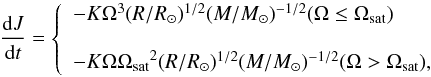 (1)where the constant K is correlated with the magnetic field strength, which is commonly taken to be a constant in all stars. Ωsat is the angular velocity at which saturation occurs, which is adjustable in the model. Following Bouvier et al. (1997), we set K = 2.0 ×1047gcm2s and Ωsat = 14 Ω⊙.
3.3. Extra-mixing in the radiative region
Microscopic diffusion and rotation-induced mixing are considered in the radiative region. The transport of angular momentum and element mixing can be described using two diffusion equations as follows (Chaboyer et al. 1995):
![\begin{eqnarray} &&\rho {r^2}\frac{I}{M}\frac{{{\rm d}\Omega }}{{{\rm d}t}} = \frac{{\rm d}}{{{\rm d}r}}\left(\rho {r^2}\frac{I}{M}{D_{\rm rot}} \frac{{{\rm d}\Omega }}{{{\rm d}t}}\right), \\ &&\rho {r^2}\frac{{{\rm d}{X_i}}}{{{\rm d}t}} = \frac{{\rm d}}{{{\rm d}r}}\left[\rho {r^2}{D_{\rm m,1}}{X_i} + \rho {r^2}({D_{\rm m,2}} + {f_{\rm c}}{D_{\rm rot}})\frac{{{\rm d}{X_i}}}{{{\rm d}t}}\right], \end{eqnarray}](/articles/aa/full_html/2014/03/aa23277-13/aa23277-13-eq64.png) where Ω is the angular velocity, Xi is the mass fraction of chemical species i, and I/M is the moment of inertia per unit mass. Dm,1 and Dm,2 are derived from the microscopic diffusion coefficients. Drot is the diffusion coefficient due to rotation-induced mixing. The details of these three parameters can be found in Chaboyer et al. (1995). The adjustable parameter fc was used to modify the effects of element mixing caused by rotation. It was determined by requiring that the lithium depletion in the solar model matches the observed depletion (Chaboyer et al. 1995).
where Ω is the angular velocity, Xi is the mass fraction of chemical species i, and I/M is the moment of inertia per unit mass. Dm,1 and Dm,2 are derived from the microscopic diffusion coefficients. Drot is the diffusion coefficient due to rotation-induced mixing. The details of these three parameters can be found in Chaboyer et al. (1995). The adjustable parameter fc was used to modify the effects of element mixing caused by rotation. It was determined by requiring that the lithium depletion in the solar model matches the observed depletion (Chaboyer et al. 1995).
4. Results
Our study is based on four observed properties (Teff, L/L⊙, log N(Li), and Prot). They were considered to limit the parameters of each of the three stars as constraints. Furthermore, seismic analyses were carried out to match the observed ⟨ Δν ⟩ and νn,ℓ).
4.1. Stellar models
To avoid unnecessary repetitions, we take star C1 as an example.
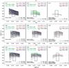 |
Fig. 1 Evolutionary tracks of the stars in the H-R diagram constrained by different observations. The top panel indicates the stellar models of C1, the middle panel those of C2, and the bottom panel those of C3. The observational constraints are effective temperature and luminosity (left panel), added lithium abundance (middle panel), and added rotational rate (right panel) for each star. The solid line presents α = 1.75 and the dashed line presents α = 1.95. The different colors represent rotating models with different initial velocities. |
Firstly, we computed the evolutionary tracks with all possible values of all input parameters. All of the evolutionary tracks in the H-R diagram are plotted in Fig. 1a1 with different line styles and colors. In this step, 280 tracks are found in the ranges of α from 1.75 to 1.95 and VZAMS from 30 to 50 km s-1. According to Fig. 1a1, we estimate the mass and age of 1.34 ± 0.11 M⊙ and 4.50 ± 1.37 Gyr for C1. We used the same observational constraints as Creevey et al. (2012), but not all of the tracks fall in the error box. This result is caused by element transport due to the interaction between rotational mixing and diffusion in the radiative region of the stellar interior (Chaboyer et al. 1995; Eggenberger et al. 2010). This type of element transport causes the rotating models to exhibit higher values of effective temperature and luminosity than models without rotation.
Then, the lithium abundance was used as a tracer to constrain the mass and age of the star. Lithium is a key element because it is easily destroyed in the stellar interiors. Its abundance indicates the amount of internal mixing in the stars, and its destruction is strongly mass- and age-dependent (do Nascimento et al. 2009; Li et al. 2012). Since lithium abundance is considered as a constraint, there are 30 tracks that fit the observed lithium abundance log N(Li). The mixing-length of all these tracks is 1.75, which can be seen in Fig. 1b1. Because the mixing-length indicates the transfer efficiency of energy and material, the lithium abundance is a function of the mixing-length. Another estimate of mass and age was obtained, which is 1.29 ± 0.06 M⊙ and 4.92 ± 0.87 Gyr. Moreover, since the lithium abundance additionally constraints the range of input parameters, the position of the star in the H-R diagram is restricted to a smaller range than in Fig. 1a1.
Furthermore, under the constraint of rotational periods, only seven tracks matched the observed Prot and are plotted in Fig. 1c1. The VZAMS is also significantly reduced to the range from 40 km s-1 to 50 km s-1. As shown in Fig. 1c1, the double constraints of lithium abundance and rotational period narrow the ranges of input parameters of the stellar models. The consideration of Prot helped us estimate mass and age of C1 even more accurately, they are 1.24 ± 0.01 M⊙ and 5.54 ± 0.21 Gyr.
The same method was used for the two other stars C2 and C3; their evolutionary tracks are plotted in Fig. 1a2 to 1c2 for C2 and in Fig. 1a3 to 1c3 for C3. Comparing Fig. 1c1, 1c2, and 1c3, we note that star C2 rotates faster than C1 and C3, which is consistent with the results obtained by Li et al. (2012): the faster the star rotates, the faster the lithium dissipates. Moreover, we find that far more tracks for C2 than C1 and C3 in Fig. 1c; this is due to the absence of a lower limit of the lithium abundance for C2.
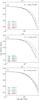 |
Fig. 2 Lithium depletion with different initial rotational rates. The different lines represent rotating models with different initial velocities. |
 |
Fig. 3 Échelle diagram corresponding to the mean value of ⟨ Δν ⟩ for C1 (Model 2), C2 (Model 9), and C3 (Model 16). The values for modes with ℓ = 0, ℓ = 1, and ℓ = 2 are shown with circles, triangles, and squares, respectively. The average large frequency separation (47.76 μHz for C1, 48.2 μHz for C2, 57.3 μHz for C3) were observed by Mathur et al. (2011) and Campante et al. (2011). |
Figure 2 plots the evolution of surface abundance of lithium with different initial rotational rates for each star. From Fig. 2, we clearly see that the surface lithium abundance generally decreases with age. When a star evolves in the MS stage, lithium depletion is caused by rotation-induced mixing. We find that rotational effects on lithium-burning in pre-MS stage are quite limited. Fast rotators exhibit almost the same lithium depletion history as slow ones. This is consistent with the results obtained in previous studies, for example, in Mendes et al. (1999). During the MS stage, fast rotators destroy more lithium than slow rotators, because they experience stronger torques and larger shears. For C1, the model of 1.23 M⊙ with VZAMS = 50 km s-1 loses about 0.8 dex lithium during the MS stage, which is 0.3 dex more than the model with VZAMS = 30 km s-1, as we can see in Fig. 2a. This trend can be reproduced in Fig. 2b for C2 and in Fig. 2c for C3. Hence, the results given by our rotating models imply that the lithium abundance can be used as a good constraint in stellar modeling.
4.2. Pulsation analysis
We used the stellar pulsation code of Guenther (1994) to perform the seismological analysis for the structure models that match all nonasteroseismic constraints. Some analytical and numerical aspects of the code are described in Guenther (1994).
The asteroseismic quantities that we considered are the mean large separation ⟨ Δν ⟩, which is defined as the differences between oscillation modes with the same angular degree and consecutive radial order n, viz., Δν(n)≡νn,ℓ − νn − 1,ℓ, and the frequencies νn,ℓ.
To fix the stellar parameters further, we performed an additional comparisons  between the theoretical and the observed stellar parameters,
 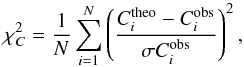 (4)where C represents the quantities Teff, L/L⊙, log g, [Fe/H], and the mean large frequency separation ⟨ Δν ⟩, Ctheo represents the theoretical values, and Cobs represents the observational values listed in Table 1. The σCobs is the errors in these observations, which are also given in Table 1.
Structure models for the seismological analysis.
Then, we compared the theoretical frequencies with observed frequencies through the function  ,
, 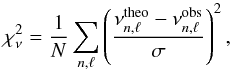 (5)where N is the total number of modes,
  and
and  are the theoretical and the observed frequencies for each spherical degree ℓ and the radial order n, and σ represents the uncertainty of the observed frequencies (Mathur et al. 2010; Campante et al. 2011).
Combining  (<1) with
  (<20), we found 17 models, viz., Model 1-5 for C1, Model 6-11 for C2, and Model 12-17 for C3, which probably are the best-fitting models. The details of all of the selected models of the three stars are shown in Table 3. The properties of the 17 models provide the final estimates of the stellar parameters of the three stars. The pulsation analysis provides even better estimates of the mass and age, which are 1.24 ± 0.01 M⊙ and 5.55 ± 0.20 Gyr for C1, 1.19 ± 0.04 M⊙ and 4.36 ± 0.29 Gyr for C2, and 1.15 ± 0.03 M⊙ and 5.68 ± 0.30 Gyr for C3.
Comparison of observed and theoretical frequencies for C1 (Model 2), C2 (Model 9), and C3 (Model 16).
Stellar parameters of the three stars determined by different methods and previous studies.
Among these models, we chose the one with the lowest value of  for each star, viz., Model 2, Model 9, and Model 16. We compare the observational and theoretical frequencies of the three models in Table 4. In addition, their échelle diagrams are plotted in Fig. 3. We note that the mixed characteristics of the mode with ℓ = 1 are fuzzy for the theoretical frequencies of all three stars. This may be because the interior structure of the star has been changed by rotation-induced mixing of elements, for instance, the size of the inner core and the stellar mean density. Hence, we might need to consider some other physical processes in detail in our future work.
5. Discussion and conclusions
Based on general observed features, we used two additional observed quantities, the lithium abundance and the rotational period, to better estimate the stellar parameters and address the problem of the incompatibility between the lithium abundance and the age in stars C1 and C3. Therefore, theoretical analyses of these two additional features can significantly constrain the ranges of the input parameters and ensure a better self-consistent stellar model.
To make our method clear and easy to compare with Creevey et al. (2012), according to the results in Fig. 1. we summarized the stellar parameters of the three stars determined by different constraints in Table 5. Previous results are listed in line 1 for each star, lines 2−5 show the stellar parameters derived in each step of our method. First, we estimated the mass and age of the stars using only the classical features Teff and L/L⊙. The uncertainty of the results is approximately 0.08 M⊙ and 1.10 Gyr. Additionally, we note that our results are not identical to those obtained by Creevey et al. (2012). The differences are caused by element transport due to the interaction between rotational mixing and diffusion in the radiative region of the stellar interior, which causes rotating models to have a higher Teff and luminosity. Because we added the lithium abundance and rotational period to our analysis, more accurate determinations were obtained. The lithium abundance helped us to improve the uncertainty of mass and age to 0.06 M⊙ and 0.90 Gyr. Next, based on the above results, we used the rotational period to constrain stellar parameters. Very precise estimates were obtained in this step, specifically, ΔM ~ 0.04 M⊙ and Δø ~ 0.50 Gyr. Finally, the pulsation analysis was performed.
After this analysis, we gave the final estimates for mass and age of the three stars, which are 1.24 ± 0.01 M⊙ and 5.55 ± 0.20 Gyr for C1, 1.19 ± 0.04 M⊙ and 4.36 ± 0.29 Gyr for C2, and 1.15 ± 0.03 M⊙ and 5.68 ± 0.30 Gyr for C3, respectively. The results locate the stars more precisely in the H-R diagram. This result is reasonable because lithium depletes as a function of mass, metallicity, rotational rates and age, while the rotational period decreases with age during the main sequence. Therefore, these two additional features can significantly constrain the input parameter ranges and improve the self-consistency and accuracy of the stellar model.
In addition, the change of the initial velocity causes different degrees of rotation-mixing in the radiative region, resulting in different processes of lithium depletion. Thus, the rotating model can be used to explain the incompatibility between lithium abundance and age in stars C1 and C3. We conclude that the lithium depletion, rotating evolution, and pulsation analysis are important to place constraints on the stellar fundamental parameters.
We will study the mixed modes of the three stars in our next work.
Acknowledgments
We are grateful to the Kepler Science Team for their constructive suggestions and valuable remarks to improve the manuscript. Funding for this Discovery mission is provided by NASA’s Science Mission Directorate. This work is supported by grants 10933002 and 11273007 from the National Natural Science Foundation of China, and the Fundamental Research Funds for the Central Universities.
References
- Angulo, C., Arnould, M., Rayet, M., et al. 1999, Nucl. Phys. A, 656, 3 [NASA ADS] [CrossRef] [Google Scholar]
- Biazzo, K., Randich, S., & Palla, F. 2011, A&A, 525, A35 [NASA ADS] [CrossRef] [EDP Sciences] [Google Scholar]
- Böhm-Vitense, E. 1958, ZAp, 46, 108 [NASA ADS] [Google Scholar]
- Bouvier, J., Forestini, M., & Allain, S. 1997, A&A, 326, 1023 [NASA ADS] [Google Scholar]
- Bruntt, H., Bedding, T. R., Quirion, P. O., et al. 2010, MNRAS, 405, 1907 [NASA ADS] [Google Scholar]
- Campante, T. L., Handberg, R., Mathur, S., et al. 2011, A&A, 534, A6 [NASA ADS] [CrossRef] [EDP Sciences] [Google Scholar]
- Castro, M., do Nascimento, J. D., Jr., Biazzo, K., et al. 2011, A&A, 526, A17 [NASA ADS] [CrossRef] [EDP Sciences] [Google Scholar]
- Chaboyer, B., Demarque, P., Guenther, D. B., et al. 1995, ApJ, 446, 435 [NASA ADS] [CrossRef] [Google Scholar]
- Creevey, O. L., Doǧan, G., Frasca, A., et al. 2012, A&A, 537, A111 [NASA ADS] [CrossRef] [EDP Sciences] [Google Scholar]
- Demarque, P., Guenther, D. B., Li, L. H., Mazumdar, A., & Straka, C. W. 2008, Ap&SS, 316, 31 [NASA ADS] [CrossRef] [Google Scholar]
- do Nascimento, J. D., Jr., Castro, M., Meléndez, J., et. al. 2009, A&A, 501, 687 [NASA ADS] [CrossRef] [EDP Sciences] [Google Scholar]
- Eggenberger, P., Meynet, G., Maeder, A., et al. 2010, A&A, 519, A116 [NASA ADS] [CrossRef] [EDP Sciences] [Google Scholar]
- Ferguson, J. W., Alexander, D. R., Allard, F., et al. 2005, ApJ, 623, 585 [NASA ADS] [CrossRef] [Google Scholar]
- Frasca, A., Guillout, P., Marilli, E., et al. 2006, A&A, 454, 301 [NASA ADS] [CrossRef] [EDP Sciences] [Google Scholar]
- García, R. A., Hekker, S., Stello, D., et al. 2011, MNRAS, 414, L6 [NASA ADS] [CrossRef] [Google Scholar]
- Gilliland, R. L., Jenkins, J. M., Borucki, W. J., et al. 2010, ApJ, 713, 160 [Google Scholar]
- Grevesse, N., & Sauval, A. J. 1998, Space Sci. Rev., 85, 161 [NASA ADS] [CrossRef] [Google Scholar]
- Guenther, D. B. 1994, ApJ, 422, 400 [NASA ADS] [CrossRef] [Google Scholar]
- Huber, D., Matthews, J. M., Croll, B., et al. 2010, ApJ, 723, 1607 [NASA ADS] [CrossRef] [Google Scholar]
- Jenkins, J. M., Caldwell, D. A., Chandrasekaran, H., et al. 2010, ApJ, 713, L87 [NASA ADS] [CrossRef] [Google Scholar]
- Kawaler, S. D. 1988, ApJ, 333, 236 [NASA ADS] [CrossRef] [Google Scholar]
- Li, T. D., Bi, S. L., Chen, Y. Q., et al. 2012, ApJ, 746, 143 [NASA ADS] [CrossRef] [Google Scholar]
- Mathur, S., García, R. A., Régulo, C., et al. 2010, A&A, 511, A46 [NASA ADS] [CrossRef] [EDP Sciences] [Google Scholar]
- Mathur, S., Handberg, R., Campante, T. L., et al. 2011, ApJ, 733, 95 [NASA ADS] [CrossRef] [Google Scholar]
- Mendes, L. T. S., D’Antona, F., & Mazzitelli, I. 1999, A&A, 341, 174 [NASA ADS] [Google Scholar]
- Niemczura, E., & Połubek, G. 2005, Mem. Soc. Astron. It., 8, 210 [Google Scholar]
- Pinsonneault, M. H., Kawaler, S. D., & Demarque, P. 1990, ApJS, 74, 501 [NASA ADS] [CrossRef] [Google Scholar]
- Pinsonneault, M. H., Deliyannis, C. P., & Demarque, P. 1992, ApJS, 78, 179 [NASA ADS] [CrossRef] [Google Scholar]
- Rogers, F. J., & Nayfonov, A. 2002, ApJ, 576, 1064 [Google Scholar]
- Sestito, P., & Randich, S. 2005, A&A, 442, 615 [NASA ADS] [CrossRef] [EDP Sciences] [Google Scholar]
- Sneden, C. 1973, ApJ, 184, 839 [NASA ADS] [CrossRef] [Google Scholar]
- Sousa, S. G., Santos, N. C., Israelian, G., Mayor, M., & Monteiro, M. J. P. F. G. 2007, A&A, 469, 783 [NASA ADS] [CrossRef] [EDP Sciences] [Google Scholar]
- Sousa, S. G., Santos, N. C., Mayor, M., et al. 2008, A&A, 487, 373 [NASA ADS] [CrossRef] [EDP Sciences] [MathSciNet] [Google Scholar]
- Thoul, A. A., Bahcall, J. N., & Loeb, A. 1994, ApJ, 421, 828 [NASA ADS] [CrossRef] [Google Scholar]
All Tables
Comparison of observed and theoretical frequencies for C1 (Model 2), C2 (Model 9), and C3 (Model 16).
Stellar parameters of the three stars determined by different methods and previous studies.
All Figures
|
Fig. 1 Evolutionary tracks of the stars in the H-R diagram constrained by different observations. The top panel indicates the stellar models of C1, the middle panel those of C2, and the bottom panel those of C3. The observational constraints are effective temperature and luminosity (left panel), added lithium abundance (middle panel), and added rotational rate (right panel) for each star. The solid line presents α = 1.75 and the dashed line presents α = 1.95. The different colors represent rotating models with different initial velocities. |
| In the text | |
|
Fig. 2 Lithium depletion with different initial rotational rates. The different lines represent rotating models with different initial velocities. |
| In the text | |
|
Fig. 3 Échelle diagram corresponding to the mean value of ⟨ Δν ⟩ for C1 (Model 2), C2 (Model 9), and C3 (Model 16). The values for modes with ℓ = 0, ℓ = 1, and ℓ = 2 are shown with circles, triangles, and squares, respectively. The average large frequency separation (47.76 μHz for C1, 48.2 μHz for C2, 57.3 μHz for C3) were observed by Mathur et al. (2011) and Campante et al. (2011). |
| In the text | |
Current usage metrics show cumulative count of Article Views (full-text article views including HTML views, PDF and ePub downloads, according to the available data) and Abstracts Views on Vision4Press platform.
Data correspond to usage on the plateform after 2015. The current usage metrics is available 48-96 hours after online publication and is updated daily on week days.
Initial download of the metrics may take a while.