| Issue |
A&A
Volume 563, March 2014
|
|
|---|---|---|
| Article Number | A104 | |
| Number of page(s) | 6 | |
| Section | Astrophysical processes | |
| DOI | https://doi.org/10.1051/0004-6361/201323087 | |
| Published online | 17 March 2014 | |
Research Note
Doppler-beaming in the Kepler light curve of LHS 6343 A
1
Institut de Ciències de l’Espai (CSIC-IEEC), Campus UAB, Facultat de
Ciències,
Torre C5 parell, 2a pl,
08193
Bellaterra,
Spain
e-mail: eherrero@ice.cat; iribas@ice.cat; morales@ice.cat
2
INAF - Osservatorio Astrofisico di Catania, via S. Sofia 78,
95123
Catania,
Italy
e-mail:
nuccio.lanza@oact.inaf.it
3
Dept. d’Astronomia i Meteorologia, Institut de Ciències del Cosmos
(ICC), Universitat de Barcelona (IEEC-UB), Martí Franquès 1, 08028
Barcelona,
Spain
e-mail:
carme.jordi@ub.edu
4
SUPA, School of Physics and Astronomy, University of St. Andrews,
North Haugh
KY16 9SS,
UK
e-mail:
acc4@st-andrews.ac.uk
5
LESIA-Observatoire de Paris, CNRS, UPMC Univ. Paris 06, Univ. Paris-Diderot, 5 Pl. Jules
Janssen, 92195
Meudon Cedex,
France
e-mail:
Juan-Carlos.Morales@obspm.fr
Received:
19
November
2013
Accepted:
18
February
2014
Context. Kepler observations revealed a brown dwarf eclipsing the M-type star LHS 6343 A with a period of 12.71 days. In addition, an out-of-eclipse light modulation with the same period and a relative semi-amplitude of ~2 × 10⁻⁴ was observed showing an almost constant phase lag to the eclipses produced by the brown dwarf. In a previous work, we concluded that this was due to the light modulation induced by photospheric active regions in LHS 6343 A.
Aims. In the present work, we prove that most of the out-of-eclipse light modulation is caused by the Doppler-beaming induced by the orbital motion of the primary star.
Methods. We introduce a model of the Doppler-beaming for an eccentric orbit and also considered the ellipsoidal effect. The data were fitted using a Bayesian approach implemented through a Markov chain Monte Carlo method. Model residuals were analysed by searching for periodicities using a Lomb-Scargle periodogram.
Results. For the first seven quarters of Kepler observations and the orbit previously derived from the radial velocity measurements, we show that the light modulation of the system outside eclipses is dominated by the Doppler-beaming effect. A period search performed on the residuals shows a significant periodicity of 42.5 ± 3.2 days with a false-alarm probability of 5 × 10⁻⁴, probably associated with the rotational modulation of the primary component.
Key words: stars: late-type / stars: rotation / binaries: eclipsing / brown dwarfs
© ESO, 2014
1. Introduction
In addition to the detection of Earth-like exoplanets, the highly accurate photometry provided by the Kepler mission has allowed the community to discover a number of eclipsing binaries and study stellar variability at very low amplitudes. Several detections of flux modulations in binary stars have been associated with relativistic beaming caused by the radial motion of their components (van Kerkwijk et al. 2010; Bloemen et al. 2011). The effect is proportional to the orbital velocity of the component stars and allows one to estimate their radial velocity amplitudes in selected compact binaries. This photometric method to measure radial velocities was first introduced by Shakura & Postnov (1987) and applied by Maxted et al. (2000). In the context of a possible application to CoRoT and Kepler light curves, it was first discussed by Loeb & Gaudi (2003) and Zucker et al. (2007).
In this paper, we present an interpretation of the out-of-eclipse light modulation in the Kepler photometry of LHS 6343 (KID 010002261) in terms of a Doppler-beaming effect. This eclipsing binary consists of an M4V star (component A) and a brown dwarf (62.7 MJup, component C) and was discovered by Johnson et al. (2011) as part of the system LHS 6343 AB, a visual binary consisting of two M-dwarf stars with a projected separation of 0.̋55. Herrero et al. (2013) analysed a more extended Kepler time series, which revealed a modulation in the flux of LHS 6343 A, synchronized with the brown dwarf orbital motion with a minimum preceding the subcompanion point by ~100°. These oscillations were assumed to be caused by persistent groups of starspots. A maximum-entropy spot-modelling technique was applied to extract the primary star rotation period, the typical lifetime of the spot, and some evidence of a possible magnetic interaction to account for the close synchronicity and almost constant phase lag between the modulation and the eclipses.
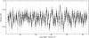 |
Fig. 1 Out-of-eclipse Kepler light curve of LHS 6343 A, covering the first seven quarters, after detrending and flux dilution correction as adopted for the subsequent analysis. |
The Doppler-beaming modelling that we present in this paper shows that the main modulation signal can instead be explained by this effect, and that the radial velocity amplitude as derived from the light curve is compatible with the spectroscopically determined value (Johnson et al. 2011). Doppler-beaming has been previously detected in Kepler light curves of KOI-74 and KOI-81 by van Kerkwijk et al. (2010), KPD 1946+4340 by Bloemen et al. (2011), KIC 10657664 by Carter et al. (2011) and KOI 1224 by Breton et al. (2012). A proper modelling of the effects observed in the light curves of these objects is important because it may give us the opportunity to derive radial velocities from a number of binaries observed by Kepler and to remove the Doppler-beaming modulation to investigate other causes of light-curve variation.
2. Photometry
LHS 6343 (KIC 010002261) was observed by Kepler during its entire mission lifetime. In this work, we re-analyse the same time series as in Herrero et al. (2013), consisting of the first seven quarters of observations (Q0 to Q6). The time series consists of a total of 22 976 data points with ~30 min cadence, a mean relative precision of 7 × 10⁻⁵, and spans ~510 days ranging from May 2009 to September 2010. The two M-type components A and B of the visual binary, separated by 0.̋55 (Johnson et al. 2011), are contained inside a single pixel of the Kepler images (the pixel side being 3.̋98), and hence any photometric mask selected for the A component contains contamination from component B.
Co-trending basis vectors are applied to the raw data using the PyKE pipeline reduction software1 to correct for systematic trends, which are mainly related to the pointing jitter of the satellite, detector instabilities, and environment variations (Murphy 2012). These are optimised tasks to reduce Kepler simple aperture photometry (SAP) data2 because they account for the position of the specific target on the detector plane to correct for systematics. From two to four vectors are used for each quarter to remove the main trends from the raw data. A low-order (≤ 4) polynomial filtering is then applied to the resulting data for each quarter because some residual trends still remain, which are followed by discontinuities between quarters. These are due to the change of the target position on the focal plane following each re-orientation of the spacecraft at the end of each quarter. As a consequence of this data reduction process, the general trends disappear, and the use of low-order polynomials ensures that the frequency and amplitude of any variability with a time scale ≲ 50 days is preserved. Several gaps in the data prevent us from using other detrending methods such as Fourier filtering (cf., Herrero et al. 2013).
The contamination from component B was corrected by subtracting its flux contribution before modelling the light curve. Johnson et al. (2011) used independent Johnson-V photometry of the A and B components together with stellar models to estimate the magnitude difference in the Kepler passband, obtaining ΔKP = 0.74 ± 0.10. This is equivalent to a flux ratio of 1.97 ± 0.19, which was applied to correct for the flux dilution produced by component B. Finally, eclipses were removed from the data set considering the ephemeris and the system parameters in Herrero et al. (2013). A complete analysis of the photometry of the brown dwarf eclipses can be found in Johnson et al. (2011) and Herrero et al. (2013). The de-trended out-of-eclipse light curve is shown in Fig. 1, while raw SAP data have been presented in Fig. 1 of Herrero et al. (2013).
3. Models of the Doppler-beaming and ellipticity effect
A first-order approximation in vR/c
for the flux variation at frequency ν due to Doppler-beaming is (cf. Rybicki & Lightman 1979; Zucker et al. 2007) 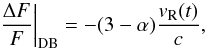 (1)where vR(t) is the radial
velocity of the star at time t, c the speed of light, and the spectral index
α ≡ dlnFν/dlnν
depends on the spectrum of the star Fν. Doppler-beaming
produces an increase of the bolometric flux for a source that is approaching the observer,
that is, when vR < 0. In the
case of LHS 6343 A, the Doppler shift of the radiation towards the blue when the star is
approaching the observer causes the flux in the Kepler passband to increase
because we observe photons with a longer wavelength in the rest frame of the source, which
corresponds to a higher flux, given the low effective temperature of the star
(Teff ~ 3000 K). In other words,
α < 0 for a star as cool as LHS
6343 A.
(1)where vR(t) is the radial
velocity of the star at time t, c the speed of light, and the spectral index
α ≡ dlnFν/dlnν
depends on the spectrum of the star Fν. Doppler-beaming
produces an increase of the bolometric flux for a source that is approaching the observer,
that is, when vR < 0. In the
case of LHS 6343 A, the Doppler shift of the radiation towards the blue when the star is
approaching the observer causes the flux in the Kepler passband to increase
because we observe photons with a longer wavelength in the rest frame of the source, which
corresponds to a higher flux, given the low effective temperature of the star
(Teff ~ 3000 K). In other words,
α < 0 for a star as cool as LHS
6343 A.
We computed a mean spectral index by integrating BT-Settl model spectra (Allard et al. 2011) over the photon-weighted
Kepler passband, 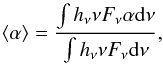 (2)where
hν is the response function
of the Kepler passband. For the stellar model Fν we assumed solar
metallicity, Teff = 3130 K, log g = 4.851
(cm s-2) and an
α-element
enhancement [α/H] = 0. The resulting mean
spectral index to be used in Eq. (1) is
⟨ α ⟩ = −3.14 ± 0.08. The uncertainty comes from the
dependence of the spectral index on the model spectrum and the uncertainties of the
respective parameters and is evaluated by calculating the integral in Eq. (2) by varying the temperature in the range
Teff = 3130 ± 20 K and the surface gravity
in log g = 4.851 ± 0.008 (cm s-2) (Johnson et al. 2011). If we compute the spectral index considering the black-body
approximation (Zucker et al. 2007), the result is
⟨ αBB ⟩ ≃ −4.22 for the Kepler
passband. The difference is due to the many absorption features in the spectrum of
this type of stars that fall within the Kepler passband.
(2)where
hν is the response function
of the Kepler passband. For the stellar model Fν we assumed solar
metallicity, Teff = 3130 K, log g = 4.851
(cm s-2) and an
α-element
enhancement [α/H] = 0. The resulting mean
spectral index to be used in Eq. (1) is
⟨ α ⟩ = −3.14 ± 0.08. The uncertainty comes from the
dependence of the spectral index on the model spectrum and the uncertainties of the
respective parameters and is evaluated by calculating the integral in Eq. (2) by varying the temperature in the range
Teff = 3130 ± 20 K and the surface gravity
in log g = 4.851 ± 0.008 (cm s-2) (Johnson et al. 2011). If we compute the spectral index considering the black-body
approximation (Zucker et al. 2007), the result is
⟨ αBB ⟩ ≃ −4.22 for the Kepler
passband. The difference is due to the many absorption features in the spectrum of
this type of stars that fall within the Kepler passband.
Assuming a reference frame with the origin at the barycentre of the binary system and the
z-axis
pointing away from the observer, we can express the radial velocity of the primary component
as a trigonometric series in the mean anomaly M by applying the elliptic expansions reported in
Murray & Dermott (1999): ![\begin{eqnarray} v_{\rm R} & = & A\left[\left(1- \frac{9e^{2}}{8}\right) \cos M + \left(e - \frac{4e^{3}}{3} \right) \cos 2M \right. \nonumber \\[1.5mm] & & + \left. \frac{9e^{2}}{8} \cos 3M + \frac{4e^{3}}{3} \cos 4M \right] \nonumber \\[1.5mm] && + B \left[ \left(1- \frac{7e^{2}}{8}\right) \sin M + \left(e - \frac{7e^{3}}{6} \right) \sin 2M \right. \nonumber \\[1.5mm] & & \left. + \frac{9e^{2}}{8} \sin 3M + \frac{4e^{3}}{3} \sin 4M \right] + O \left(e^{4}\right), \label{vr_eq} \end{eqnarray}](/articles/aa/full_html/2014/03/aa23087-13/aa23087-13-eq38.png) (3)where
A ≡ Kcosω and
B ≡ −Ksinω, with
K the radial
velocity semi-amplitude, ω the argument of periastron, and e the eccentricity of the
orbit of the primary component (see, e.g., Wright &
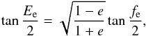
Howard 2009). At the epoch of mid-eclipse of the primary by the brown dwarf, the
true anomaly is (cf., e.g., Winn 2011):
(3)where
A ≡ Kcosω and
B ≡ −Ksinω, with
K the radial
velocity semi-amplitude, ω the argument of periastron, and e the eccentricity of the
orbit of the primary component (see, e.g., Wright &
Howard 2009). At the epoch of mid-eclipse of the primary by the brown dwarf, the
true anomaly is (cf., e.g., Winn 2011):
 . From the true anomaly at
mid-eclipse, we find the eccentric anomaly and the mean anomaly:
. From the true anomaly at
mid-eclipse, we find the eccentric anomaly and the mean anomaly:
 (4)and
 (5)If we measure the time
since the mid-eclipse epoch T0, the mean anomaly appearing in Eq.
(3) is
(5)If we measure the time
since the mid-eclipse epoch T0, the mean anomaly appearing in Eq.
(3) is
 (6)because M is zero at the epoch of
periastron.
(6)because M is zero at the epoch of
periastron.
In addition to the Doppler-beaming effect, the ellipsoidal effect can be important in the
case of LHS 6343 A, while the reflection effect is negligible because of a relative
separation of ~45.3 stellar
radii in the system and the low luminosity of the C secondary component. Morris (1985) provided formulae to evaluate the effect.
In our case, only the coefficient proportional to cos2φ, where φ = M − Me
is the orbital angular phase, is relevant because the other terms are at least one order of
magnitude smaller due to the large relative separation. In terms of the mean anomaly, the
relative flux modulation due to the ellipsoidal effect is ![\begin{eqnarray} \left.\frac{\Delta F}{F}\right|_{\rm E} & = & C_{1}(2) \cos \left(2M -2M_{\rm e}\right) \nonumber \\[1.5mm] & = & \left[C_{1}(2)\sin\left(2M_{\rm e}\right)\right]\sin 2M + \left[C_{1}(2)\cos\left(2M_{\rm e}\right)\right] \cos 2M, \nonumber \\ \label{elip1} \end{eqnarray}](/articles/aa/full_html/2014/03/aa23087-13/aa23087-13-eq52.png) (7)where
(7)where
 (8)m is the mass of the brown
dwarf secondary, M∗ the mass of the distorted primary star,
R its radius,
and i the
inclination of the orbital plane, which are fixed to those derived by Johnson et al. (2011). Finally, Z1(2) is a coefficient given by
(8)m is the mass of the brown
dwarf secondary, M∗ the mass of the distorted primary star,
R its radius,
and i the
inclination of the orbital plane, which are fixed to those derived by Johnson et al. (2011). Finally, Z1(2) is a coefficient given by
 (9)where u = 1.2 is the linear
limb-darkening coefficient in the Kepler passband, τg ~ 0.32 the
gravity-darkening coefficient estimated for the primary LHS 6343 A, and we neglected the
effects related to the precession constant and the (small) eccentricity of the orbit (cf.,
Morris 1985). Note that at mid-eclipse,
M = Me, and the
ellipsoidal variation is at a minimum, while for M = Me ± π/2,
that is, in quadrature, it reaches a maximum.
(9)where u = 1.2 is the linear
limb-darkening coefficient in the Kepler passband, τg ~ 0.32 the
gravity-darkening coefficient estimated for the primary LHS 6343 A, and we neglected the
effects related to the precession constant and the (small) eccentricity of the orbit (cf.,
Morris 1985). Note that at mid-eclipse,
M = Me, and the
ellipsoidal variation is at a minimum, while for M = Me ± π/2,
that is, in quadrature, it reaches a maximum.
In conclusion, the total relative light variation due to both Doppler-beaming and
ellipsoidal effect is  (10)
(10)
4. Results
To fit the proposed model to the data, we applied a Markov chain Monte Carlo (MCMC)
approach that allowed us to find, in addition to the best-fit solution, the posterior
distribution of the parameters that provides us with their uncertainties and correlations.
We followed the method outlined in Appendix A of Sajina et
al. (2006) (see also Press et al. 2002;
Ford 2006). If a ≡ { e,ω,K } is the
vector of the parameter values, and d the vector of the data points,
according to the Bayes theorem we have  (11)where p(a|d)
is the a posteriori probability distribution of the parameters, p(d|a)
the likelihood of the data for the given model, and p(a) the prior. In our
case, the parameters have been derived by Johnson et al.
(2011) by fitting the radial velocity and transit light-curves. Therefore, we can
use their values and uncertainties to define the prior as
(11)where p(a|d)
is the a posteriori probability distribution of the parameters, p(d|a)
the likelihood of the data for the given model, and p(a) the prior. In our
case, the parameters have been derived by Johnson et al.
(2011) by fitting the radial velocity and transit light-curves. Therefore, we can
use their values and uncertainties to define the prior as ![\begin{eqnarray} p(\vec a) & = &\exp\left\{ -\left[\frac{(e-0.056)}{0.032} \right]^{2} - \left[\frac{(\omega +23)}{56} \right]^{2} \right. \nonumber \\[1.5mm] & & \left. - \left[ \frac{(K-9.6)}{0.3} \right]^{2} \right\}, \label{prior} \end{eqnarray}](/articles/aa/full_html/2014/03/aa23087-13/aa23087-13-eq71.png) (12)where
ω is measured
in degrees and K in km s-1. The likelihood of the data for given model parameters
is
(12)where
ω is measured
in degrees and K in km s-1. The likelihood of the data for given model parameters
is  (13)where
 is the reduced
chi-square of the fit to the data obtained with our model. The standard deviation of the
data used to compute is the mean of
the standard deviations evaluated in 40 equal bins of the mean anomaly and is
σm = 2.057 × 10⁻⁴ in relative
flux units. Note that in addition to estimating the standard deviation of the data, we
always fitted the unbinned time-series shown in Fig. 1.
Substituting Eqs. (13) and (12) into Eq. (11), we obtain the posterior probability distribution of the parameters.
We sampled from this distribution by means of the Metropolis-Hasting algorithm (cf., e.g.,
Press et al. 2002), thus avoiding the complicated
problem of normalizing p(a|d)
over a multi-dimensional parameter space. A MCMC is built by performing a conditioned random
walk within the parameter space. Specifically, starting from a given point ai, a proposal
is made to move to a successive point ai + 1
whose coordinates are found by incrementing those of the initial point by random deviates
taken from a multi-dimensional Gaussian distribution with standard deviations
σj, where j = 1, 2 or 3 indicate the
parameter. With this choice for the proposed increments of the parameters, the step is
accepted if p(ai + 1|d)/p(ai|d) > u,
where u is a
random number between 0 and 1 drawn from a uniform distribution, otherwise we return to the
previous point, that is, ai + 1 = ai.
is the reduced
chi-square of the fit to the data obtained with our model. The standard deviation of the
data used to compute is the mean of
the standard deviations evaluated in 40 equal bins of the mean anomaly and is
σm = 2.057 × 10⁻⁴ in relative
flux units. Note that in addition to estimating the standard deviation of the data, we
always fitted the unbinned time-series shown in Fig. 1.
Substituting Eqs. (13) and (12) into Eq. (11), we obtain the posterior probability distribution of the parameters.
We sampled from this distribution by means of the Metropolis-Hasting algorithm (cf., e.g.,
Press et al. 2002), thus avoiding the complicated
problem of normalizing p(a|d)
over a multi-dimensional parameter space. A MCMC is built by performing a conditioned random
walk within the parameter space. Specifically, starting from a given point ai, a proposal
is made to move to a successive point ai + 1
whose coordinates are found by incrementing those of the initial point by random deviates
taken from a multi-dimensional Gaussian distribution with standard deviations
σj, where j = 1, 2 or 3 indicate the
parameter. With this choice for the proposed increments of the parameters, the step is
accepted if p(ai + 1|d)/p(ai|d) > u,
where u is a
random number between 0 and 1 drawn from a uniform distribution, otherwise we return to the
previous point, that is, ai + 1 = ai.
We computed a chain of 200 000 points adjusting σj to have an average acceptance probability of 23 per cent that guarantees a proper sampling and minimises the internal correlation of the chain itself. The mixing and convergence of the chain to the posterior parameter distribution were tested with the method of Gelman and Rubin as implemented by Verde et al. (2003). First we discarded the first 25 000 points that correspond to the initial phase during which the Metropolis-Hasting algorithm converges on the stationary final distribution (the so-called burn-in phase), then we cut the remaining chain into four subchains that were used to compute the test parameter R. It must be lower than 1.1 when the chain has converged on the distribution to be sampled. In our case we found (R − 1) ≤ 4.4 × 10⁻⁴ for all the three parameters, which indicates convergence and good sampling of the parameter space.
The best-fit model corresponding to the minimum  has
the parameters e = 0.0448,
has
the parameters e = 0.0448,  ,
and K = 9.583
km s-1. For
comparison, the reduced chi-square corresponding to the best-fit parameters of Johnson et al. (2011) is 1.0098.
,
and K = 9.583
km s-1. For
comparison, the reduced chi-square corresponding to the best-fit parameters of Johnson et al. (2011) is 1.0098.
Our best fit to the data is plotted in Fig. 2 where
the points are binned for clarity into 40 equal intervals of mean anomaly M. The semi-amplitude of the
errorbar of each binned point is the standard error of the flux in the given bin. The
posterior distributions of the parameters are plotted in Fig. 3. The intervals enclosing between 15.9 and 84.1 per cent of the distributions are
0.035 ≤ e ≤ 0.097;
 ;
and 9.290 ≤ K ≤ 9.897 km s-1. The correlations among the
parameters are not particularly significant, as shown by the two-dimensional posterior
distributions plotted in Fig. 4. The best-fit
parameters of Johnson et al. (2011) fall within the
68.2 per cent confidence regions of our two-dimensional distributions.
;
and 9.290 ≤ K ≤ 9.897 km s-1. The correlations among the
parameters are not particularly significant, as shown by the two-dimensional posterior
distributions plotted in Fig. 4. The best-fit
parameters of Johnson et al. (2011) fall within the
68.2 per cent confidence regions of our two-dimensional distributions.
The good agreement between the data and the model demonstrates that most of the light modulation of LHS 6343 A can be accounted for by a Doppler-beaming effect with a fitted semi-amplitude of 1.963 × 10⁻⁴ in relative flux units. The contribution of the ellipsoidal effect is very small, with a relative semi-amplitude of only 3.05 × 10⁻⁶ as derived by Eqs. (7)–(9).
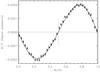 |
Fig. 2 Relative flux variation of LHS 6343 A vs. the mean anomaly M of the orbit, binned in 40 equal intervals. The Doppler-beaming plus ellipsoidal effect model for our best-fitting parameters is plotted with a solid line (cf. the text). The value of M/2π corresponding to mid-eclipse is marked with a dotted vertical segment, while a horizontal dotted line is plotted to indicate the zero-flux level. |
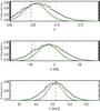 |
Fig. 3 Top panel: a posteriori distribution of eccentricity e as obtained with our MCMC approach. The vertical dashed line indicates the value corresponding to the best fit plotted in Fig. 2, while the two vertical dotted lines enclose an interval between 15.9 and 84.1 per cent of the distribution. The solid green line is the mean likelihood as computed by means of Eq. (A4) of Sajina et al. (2006), while the dashed orange line is the prior assumed for the parameter. These two distributions have been normalized to the maximum of the a posteriori distribution of the eccentricity. Note that the two distributions are very similar, indicating that fitting Doppler-beaming does not add much constraint to the eccentricity. Middle panel: as upper panel, but for the argument of periastron ω. Lower panel: as upper panel, but for the semi-amplitude of the radial velocity modulation K. |
The distribution of the residuals to our best fit is plotted in Fig. 5. It can be fitted by a Gaussian of standard deviation 1.929 × 10⁻⁴ in relative flux units, although there is an excess of residuals larger than ~4 × 10⁻⁴ in absolute value. The amplitude of the Doppler-beaming plus ellipsoidal modulation is comparable with the standard deviation of the residuals. This accounts for the quite extended confidence intervals found in the parameter distributions. In other words, the parameters derived by fitting the Doppler-beaming are of lower accuracy than those derived by fitting the spectroscopic orbit because the radial velocity measurements are more accurate. The a posteriori distributions of the fitted parameters in Fig. 3 are dominated by their priors, confirming that Doppler-beaming data do not add much information on the model parameters. As a consequence, the best-fit value of ω deviates by more than one standard deviation from the mean of its posterior distribution.
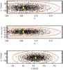 |
Fig. 4 Upper panel: two-dimensional a posteriori distribution of the argument of periastron ω vs. the eccentricity e as obtained with the MCMC method. The yellow filled circle corresponds to the best-fit orbital solution of Johnson et al. (2011), while the green circle indicates our best-fit values of the parameters. The orange level lines enclose 68.2, 95, and 99.7 per cent of the distribution, respectively. Individual points of the MCMC have been plotted after applying a thinning factor of 100 to the chain for clarity. Middle panel: as upper panel, but for the radial velocity semi-amplitude K and the eccentricity e. Lower panel: as upper panel, but for the argument of periastron ω and the radial velocity semi-amplitude K. |
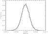 |
Fig. 5 Distribution of the residuals resulting from the Doppler-beaming plus ellipsoidal effect model of the photometric data of LHS 6343 A. The solid line is a Gaussian fit to the distribution. |
Finally, we plot in Fig. 6 the Lomb-Scargle periodogram of the residuals computed with the algorithm of Press & Rybicki (1989). We found a significant periodicity of 42.49 ± 3.22 days with a false-alarm probability (FAP) of 4.8 × 10⁻⁴ as derived by analysing 105 random permutations of the flux values with the same time-sampling. The second peak in the periodogram is not a harmonic of the main peak and has an FAP of 20.4 per cent, thus it is not considered to be reliable. The vertical dotted lines indicate the frequencies corresponding to the orbital period and its harmonics. Note that the signal at these frequencies has been almost completely removed by subtracting our model.
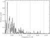 |
Fig. 6 Lomb-Scargle periodogram of the residuals resulting from the Doppler-beaming plus ellipsoidal effect model of the photometric data of LHS 6343 A. Dotted lines correspond to the frequency of the orbital period and its harmonics. |
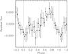 |
Fig. 7 Residuals of the Doppler-beaming plus ellipsoidal effect model of LHS 6343 A folded at a periodicity of 42.49 days. |
The residuals folded at the periodicity of 42.49 days are displayed in Fig. 7, showing the mean residual flux vs. phase in 40 equal bins. A modulation is clearly apparent, suggesting that the primary star’s rotation combined with the presence of persistent starspots might be producing this signal. The possibility that the modulation is due to pulsations seems unlikely given the long period, but cannot be completely ruled out (see, e.g., Toma 1972; Palla & Baraffe 2005, and references therein). Given the non-sinusoidal shape of the modulation, we have also considered a phasing of the residuals with half the main period (i.e., 21.102 days), but the dispersion of the points around the mean modulation is remarkably higher.
The non-synchronous rotation of the primary and the eccentricity of the orbit are consistent with time scales of tidal synchronisation and circularisation at least of the order of the main-sequence lifetime of the system as discussed by Herrero et al. (2013).
5. Conclusions
We have demonstrated that the main assumption made by Herrero et al. (2013) to explain the flux variability in LHS 6343 A as caused by the rotational modulation of photospheric active regions is incomplete. The mean amplitude and phase lag of the modulation can be accounted for by a Doppler-beaming model that agrees with the orbital parameters derived by Johnson et al. (2011) by fitting the transits and the radial velocity observations. The ellipsoidal effect was found to be virtually negligible and the reflection effect was not considered given the distance and the luminosity ratio of the two components in the system.
The periodogram of the residuals reveals a significant periodicity at ~42.5 ± 3.2 days (FAP of 4.8 × 10⁻⁴), probably related to the rotation period of LHS 6343 A. A more accurate data-detrending procedure, as is expected to be applied to the final Kepler data release, might be useful to confirm this point and extract more results from the residual analysis.
Acknowledgments
The authors are grateful to the anonymous referee for valuable comments that helped to improve their analysis. The interpretation presented in this work was originally suggested by one of us (ACC) during a seminar held at the School of Physics and Astronomy of the University of St. Andrews, UK. E.H. and I.R. acknowledge ancillary support from the Spanish Ministry of Economy and Competitiveness (MINECO) and the ”Fondo Europeo de Desarrollo Regional” (FEDER) through grant AYA2012- 39612-C03-01. C.J. acknowledges support from the /MINECO/ (Spanish Ministry of Economy) - FEDER through grant AYA2009-14648-C02-01, AYA2010-12176-E, AYA2012-39551-C02-01 and CONSOLIDER CSD2007-00050. E.H. is supported by a JAE Pre-Doc grant (CSIC).
References
- Allard, F., Homeier, D., & Freytag, B. 2011, ASP Conf. Ser., 448, 91 [NASA ADS] [Google Scholar]
- Bloemen, S., Marsh, T. R., Østensen, R. H., et al. 2011, MNRAS, 410, 1787 [NASA ADS] [Google Scholar]
- Breton, R. P., Rappaport, S. A., van Kerkwijk, M. H., & Carter, J. A. 2012, ApJ, 748, 115 [NASA ADS] [CrossRef] [Google Scholar]
- Carter, J. A., Rappaport, S., & Fabrycky, D. 2011, ApJ, 728, 139 [NASA ADS] [CrossRef] [Google Scholar]
- Ford, E. B. 2006, ApJ, 642, 505 [NASA ADS] [CrossRef] [Google Scholar]
- Herrero, E., Lanza, A. F., Ribas, I., Jordi, C., & Morales, J. C. 2013, A&A, 553, A66 [NASA ADS] [CrossRef] [EDP Sciences] [Google Scholar]
- Husnoo, N., Pont, F., Mazeh, T., et al. 2012, MNRAS, 422, 3151 [NASA ADS] [CrossRef] [Google Scholar]
- Johnson, J. A., Apps, K., Gazak, J. Z., et al. 2011, ApJ, 730, 79 [NASA ADS] [CrossRef] [Google Scholar]
- Loeb, A., & Gaudi, B. S. 2003, ApJ, 588, 117 [Google Scholar]
- Maxted, P. F. L., Marsh, T. R., North, R. C., et al. 2000, MNRAS, 317, L41 [NASA ADS] [CrossRef] [Google Scholar]
- Morris, S. L. 1985, ApJ, 295, 143 [NASA ADS] [CrossRef] [Google Scholar]
- Murphy, S. J. 2012, MNRAS, 422, 665 [NASA ADS] [CrossRef] [Google Scholar]
- Murray, C. D., & Dermott, S. F. 1999, Solar system dynamics, ed. C. D. Murray (Cambridge: Cambridge Univ. Press) [Google Scholar]
- Palla, F., & Baraffe, I. 2005, A&A, 432, L57 [NASA ADS] [CrossRef] [EDP Sciences] [Google Scholar]
- Press, W. H., & Rybicki, G. B. 1989, ApJ, 338, 277 [NASA ADS] [CrossRef] [Google Scholar]
- Press, W. H., Teukolsky, S. A., Vetterling, W. T., & Flannery, B. P. 2002, Numerical recipes in C++: the art of scientific computing (Cambridge: Cambridge Univ. Press) [Google Scholar]
- Rowe, J. F., Borucki, W. J., Koch, D., et al. 2010, ApJ, 713, L150 [NASA ADS] [CrossRef] [Google Scholar]
- Rybicki, G. B., & Lightman, A. P. 1979, Astron. Quarterly, 3, 1999 [Google Scholar]
- Sajina, A., Scott, D., Dennefeld, M., et al. 2006, MNRAS, 369, 939 [NASA ADS] [CrossRef] [Google Scholar]
- Shakura, N. I., & Postnov, K. A. 1987, A&A, 183, L21 [NASA ADS] [Google Scholar]
- Toma, E. 1972, A&A, 19, 76 [NASA ADS] [Google Scholar]
- van Kerkwijk, M. H., Rappaport, S. A., Breton, R. P., et al. 2010, ApJ, 715, 51 [NASA ADS] [CrossRef] [Google Scholar]
- Verde, L., Peiris, H. V., Spergel, D. N., et al. 2003, ApJS, 148, 195 [NASA ADS] [CrossRef] [Google Scholar]
- Winn, J. N. 2011, in Exoplanets, ed. S. Seager (Tucson: University of Arizona Press), 55 [Google Scholar]
- Wright, J. T., & Howard, A. W. 2009, ApJS, 182, 205 [NASA ADS] [CrossRef] [Google Scholar]
- Wright, J. T., & Howard, A. W. 2013, ApJS, 205, 22, Erratum [NASA ADS] [CrossRef] [Google Scholar]
- Zucker, S., Mazeh, T., & Alexander, T. 2007, ApJ, 670, 1326 [NASA ADS] [CrossRef] [Google Scholar]
All Figures
|
Fig. 1 Out-of-eclipse Kepler light curve of LHS 6343 A, covering the first seven quarters, after detrending and flux dilution correction as adopted for the subsequent analysis. |
| In the text | |
|
Fig. 2 Relative flux variation of LHS 6343 A vs. the mean anomaly M of the orbit, binned in 40 equal intervals. The Doppler-beaming plus ellipsoidal effect model for our best-fitting parameters is plotted with a solid line (cf. the text). The value of M/2π corresponding to mid-eclipse is marked with a dotted vertical segment, while a horizontal dotted line is plotted to indicate the zero-flux level. |
| In the text | |
|
Fig. 3 Top panel: a posteriori distribution of eccentricity e as obtained with our MCMC approach. The vertical dashed line indicates the value corresponding to the best fit plotted in Fig. 2, while the two vertical dotted lines enclose an interval between 15.9 and 84.1 per cent of the distribution. The solid green line is the mean likelihood as computed by means of Eq. (A4) of Sajina et al. (2006), while the dashed orange line is the prior assumed for the parameter. These two distributions have been normalized to the maximum of the a posteriori distribution of the eccentricity. Note that the two distributions are very similar, indicating that fitting Doppler-beaming does not add much constraint to the eccentricity. Middle panel: as upper panel, but for the argument of periastron ω. Lower panel: as upper panel, but for the semi-amplitude of the radial velocity modulation K. |
| In the text | |
|
Fig. 4 Upper panel: two-dimensional a posteriori distribution of the argument of periastron ω vs. the eccentricity e as obtained with the MCMC method. The yellow filled circle corresponds to the best-fit orbital solution of Johnson et al. (2011), while the green circle indicates our best-fit values of the parameters. The orange level lines enclose 68.2, 95, and 99.7 per cent of the distribution, respectively. Individual points of the MCMC have been plotted after applying a thinning factor of 100 to the chain for clarity. Middle panel: as upper panel, but for the radial velocity semi-amplitude K and the eccentricity e. Lower panel: as upper panel, but for the argument of periastron ω and the radial velocity semi-amplitude K. |
| In the text | |
|
Fig. 5 Distribution of the residuals resulting from the Doppler-beaming plus ellipsoidal effect model of the photometric data of LHS 6343 A. The solid line is a Gaussian fit to the distribution. |
| In the text | |
|
Fig. 6 Lomb-Scargle periodogram of the residuals resulting from the Doppler-beaming plus ellipsoidal effect model of the photometric data of LHS 6343 A. Dotted lines correspond to the frequency of the orbital period and its harmonics. |
| In the text | |
|
Fig. 7 Residuals of the Doppler-beaming plus ellipsoidal effect model of LHS 6343 A folded at a periodicity of 42.49 days. |
| In the text | |
Current usage metrics show cumulative count of Article Views (full-text article views including HTML views, PDF and ePub downloads, according to the available data) and Abstracts Views on Vision4Press platform.
Data correspond to usage on the plateform after 2015. The current usage metrics is available 48-96 hours after online publication and is updated daily on week days.
Initial download of the metrics may take a while.