| Issue |
A&A
Volume 563, March 2014
|
|
|---|---|---|
| Article Number | A68 | |
| Number of page(s) | 26 | |
| Section | Astrophysical processes | |
| DOI | https://doi.org/10.1051/0004-6361/201322752 | |
| Published online | 12 March 2014 | |
Star formation sites toward the Galactic center region
The correlation of CH3OH masers, H2O masers, and near-IR green sources⋆
1
I. Physikalisches Institut, Universität zu Köln,
Zülpicher Str. 77, 50937
Köln, Germany
e-mail: chambers@ph1.uni-koeln.de
2
Department of Physics and Astronomy and Center for
Interdisciplinary Research in Astronomy, Northwestern University,
Evanston
IL
60208,
USA
3
National Radio Astronomy Observatory, 1003 Lopezville Road, Socorro
NM
87801,
USA
Received: 25 September 2013
Accepted: 15 January 2014
Aims. We present a study of star formation in the central molecular zone (CMZ) of our Galaxy through the association of three star formation indicators: 6.7 GHz CH3OH masers, 22 GHz H2O masers, and enhanced 4.5 μm emission (‘green’) sources. We explore how star formation in the CMZ(|ℓ| < 1.3°, |b| < 10′) compares with that of the Galactic disk (6 °> ℓ > 345°, |b| < 2°).
Methods. Using an automated algorithm, we search for green sources toward 6.7 GHz CH3OH masers detected in the Parkes Methanol Multibeam Survey. We combine these results with lists of 22 GHz H2O masers, including our Mopra survey of the CMZ.
Results. We find that the correlation of CH3OH masers with green sources is a function of Galactic latitude, with a minimum close to b = 0 and increasing with |b| (toward the central part of the Galaxy, 6 °> ℓ > 345°, |b| < 2°). We find no significant difference between the correlation rate of CH3OH masers with green sources in the CMZ and the disk. This suggests that although the physical conditions of the gas are different in the CMZ from that of the Galactic disk, once gravitational instability sets in at sufficiently high densities, signatures of star formation appear to be similar in both regions. Moreover, the detection of green sources, even at the distance of the Galactic center, shows that our technique can easily identify the early stages of star formation, especially in low-extinction regions of the Galaxy. Through the association of H2O and CH3OH masers, we identify 15 star-forming sites in the CMZ. We find a higher correlation rate of coincident H2O and CH3OH masers within the CMZ compared to the Galactic disk, indicating a difference in the maser evolutionary sequence for star-forming cores in these two regions.
Key words: ISM: clouds / ISM: molecules / stars: formation / Galaxy: center
Appendices A and B are available in electronic form at http://www.aanda.org
© ESO, 2014
1. Introduction
As the nearest galactic nucleus, our Galactic center (GC) provides us with the opportunity to study in detail the star formation process in the extreme conditions at the centers of galaxies. The inner few hundred pc of the Galactic center, known as the central molecular zone (CMZ) contains few times 107M⊙ of molecular gas (Pierce-Price et al. 2000; Ferrière et al. 2007; Longmore et al. 2012) and hosts several prominent sites of star formation regions (e.g., Sgr A, Sgr B2 and Sgr C; see Fig. 1). By studying sites of star formation in this complex region, we can learn global characteristics of the star formation process and compare with nuclei of other galaxies.
The CMZ is characterized to be different from the Galactic disk in several ways, such as its chemistry (Martín-Pintado et al. 2000; Oka et al. 2005; Riquelme et al. 2010; Jones et al. 2011, 2012, 2013; Yusef-Zadeh et al. 2013a), a two-temperature distribution of molecular gas (e.g., Hüttemeister et al. 1998; Mills & Morris 2013), its dust temperature being lower than its gas temperature (Odenwald & Fazio 1984; Cox & Laureijs 1989; Pierce-Price et al. 2000; Ferrière et al. 2007; Molinari et al. 2011; Immer et al. 2012), stronger turbulence (cf. Morris & Serabyn 1996), and evidence that it is a region dominated by cosmic rays (Yusef-Zadeh et al. 2013a,b; Ao et al. 2013). Using thermal dust emission data from the Herschel Hi-GAL Key-Project, Molinari et al. (2011) have shown that much of this mass (~3 × 10⁷M⊙) resides in a filamentary, twisted ring-like structure that encircles the center of the Galaxy. This ring has a projected extent of ~180 pc, is comprised of a dense, cold (T ≤ 20 K) dust cloud with high column density that encloses warmer dust (T ≥ 25 K) with lower column density in the interior of the ring. The recent results of Jones et al. (2012), who used the Mopra telescope to map the CMZ in ~20 molecular transitions at ~3 mm, show that the clouds in the region display bright emission with large linewidths and profiles consisting of several velocity components, all indicating the complex kinematic structure and composition of the gas in the Galactic center zone.
While it is clear that physical characteristics of the gas are unique in the CMZ, it is not clear how star formation in this region compares to that of the Galactic disk. Assuming that the gas is distributed uniformly throughout the inner 400 pc of the Galaxy rather than in a ring geometry, the Kennicut law (Kennicutt 1998) still holds in a region where tidal shear could be important (Yusef-Zadeh et al. 2009). To make the comparison between star formation in the CMZ and in the Galactic disk, we look at the correlation of two star formation indicators-maser emission (from both CH3OH and H2O) and extended, enhanced 4.5 μm emission. Because of their different emission mechanisms, the correlation between the two can help constrain the evolutionary states of young stars.
The Class II CH3OH maser transition at 6.7 GHz is one of the brightest known maser lines and is known to be an excellent signpost of star formation (e.g., Menten 1991; Minier et al. 2003; Caswell et al. 2010). The population inversion that gives rise to the transition is thought to be radiatively pumped, presumably by a central high-mass (≥8 M⊙) protostellar object (Cragg et al. 1992). It has been shown that this maser traces only high-mass star formation (Walsh et al. 2001; Minier et al. 2003), and is typically found close to young stars (Caswell 1997; Ellingsen 2005). As such, it is used as a marker of high-mass star formation throughout the Galaxy. Another well-known signpost of star formation is the H2O maser transition at 22.23 GHz (Genzel et al. 1978; Gwinn 1994; Claussen et al. 1998; Furuya et al. 2001). The population inversion is created in shocks and outflows (Norman & Silk 1979; Elitzur et al. 1989; Hollenbach et al. 2013), and the maser is associated with both low- and high-mass star formation (as well as AGB stars and super-massive black holes), and has been the target of many recent observations and surveys (e.g., Caswell et al. 2011; Walsh et al. 2011). Many young star forming sites in the Galaxy harbor both CH3OH and H2O masers.
A more recently discovered tracer of star formation activity is extended, enhanced 4.5 μm emission, commonly known as “green fuzzies” (Chambers et al. 2009) or extended green objects (EGOs; Cyganowski et al. 2008). These sources appear green in Spitzer/IRAC (Fazio et al. 2004) 3-color images (8.0 μm in red, 4.5 μm in green, and 3.6 μm in blue). The 4.5 μm enhancement is likely due to a shock-excited H2 feature in the 4.5 μm band (Noriega-Crespo et al. 2004; De Buizer & Vacca 2010), but it could also be from a shocked CO feature (Marston et al. 2004). While its exact nature is still uncertain, this 4.5 μm emission, frequently referred to as “green” emission throughout this paper, is a reliable tracer of the early stages of star formation (Chambers et al. 2009; Cyganowski et al. 2008, 2009).
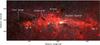 |
Fig. 1 Spitzer/IRAC 3-color image (with 8.0 μm in red, 4.5 μm in green, and 3.6 μm in blue) of the Central Molecular Zone. Some of the more prominent Galactic center features are labelled. Sgr A∗ is centered on the nuclear cluster. |
There have been several studies that show the correlation of green sources with maser emission. Yusef-Zadeh et al. (2007) found an association of green sources with 6.7 GHz CH3OH masers toward the Galactic center, and other studies have since found similar correlations in the Galactic disk, with both 6.7 GHz CH3OH and 22 GHz H2O masers (Chambers et al. 2009; Chen et al. 2009; Cyganowski et al. 2009). Using a sample of 31 green sources (15 in the CMZ, and 16 foreground to the Galactic center region), Chambers et al. (2011) searched for a difference in the correlation rate of 6.7 GHz CH3OH masers with green sources between the CMZ and the Galactic disk. They found no significant difference in the correlation rate, but that study suffered from small-number statistics.
In this paper, we search for differences in the correlation of masers with green sources between the Galactic center and the Galactic disk using a different approach. While the studies mentioned above search for maser emission toward samples of green sources, we instead search for extended, enhanced 4.5 μm emission toward 6.7 GHz CH3OH maser emission. We then correlate the results with a list of 22.23 GHz H2O masers, which is a combination of the results of our Mopra H2O maser survey of the CMZ and H2O masers identified by Caswell et al. (2011) and Walsh et al. (2011). This method has several advantages, such as a large sample of CH3OH masers from the Parkes Methanol Multibeam Survey (Caswell et al. 2010, C10 hereafter). Moreover, it uses an automated, uniform approach to identifying enhanced 4.5 μm emission. Finally, it makes use of H2O masers as a third tracer of star formation indicator. Using this method, we explore how star formation in the Galactic center compares with that of the Galactic disk and identify sites of star formation using three different tracers.
The structure of this paper is as follows. In Sect. 2, we present our Mopra H2O maser survey of the Galactic center region, along with brief descriptions of earlier surveys of H2O masers (Caswell et al. 2011; Walsh et al. 2011), CH3OH masers (C10), and the Spitzer/IRAC survey of the GC region. We describe our source detection and correlation algorighthms in Sect. 3. In Sect. 4, we present the results after the application of the method. We discuss these results in Sect. 5, and summarize our findings in Sect. 6.
2. Data
2.1. 6.7 GHz CH3OH masers
The 6.7 GHz CH3OH masers we use in our analysis were identified by C10 as part of the Parkes Methanol Multibeam Survey. Initial detections of the 6.7 GHz CH3OH masers were made with the Parkes Observatory, and subsequent follow-up observations with the Australia Telescope Compact Array to pinpoint the maser locations to 0.4′′ accuracy. The full survey covers the entire Galactic plane with a latitude range of |b| < 2°. C10 published a subset of this survey, covering 6 °> ℓ > 345°, |b| < 2° with a 1σ detection limit of 0.07 Jy.
2.2. H2O maser data
We observed the Galactic center region with the CSIRO/CASS Mopra telescope in the period 2006 Sep. 13 to 2006 Oct. 15 and 2007 July 24 to September 17. Data were taken in the on-the-fly mode, dumping data every 2 s with the then newly installed 12mm receiver, dual polarization. We observed the Galactic longitude range of −1.5° < ℓ < 2° and Galactic latitude range of |b| < 0.5°. The entire area was split into smaller, typically 18′ on-the-fly subfields that were repeatedly and alternately observed in Galactic latitude and longitude directions, at least four times.
As a reference position we observed at (ℓ,b) = (4.301°, 1.667°) after every row. The data were calibrated with an internal noise diode. At the time of the observations in 2006, however, the noise diode was not fully calibrated itself and we used the 2007 observations to obtain pointed observations in each on-the-fly field from which we re-calibrated the 2006 data. The absolute calibration is estimated to be accurate to ~20%. We used the MOPS1 backend in the mops_2208_8192_4f wideband mode to cover a large range of molecular lines, including the 22.235120 GHz rest frequency of the J = 616−523 water (H2O) transition. The full frequency coverage is 8.8 GHz (4 subbands) with 8096 channels within a 2.2 GHz subband. The data were processed with the ATNF packages livedata and gridzilla2. Livedata calibrates the spectra using ON and OFF scans and gridzilla grids all spectra into datacubes that we specified to be 0.5′ per pixel, with a FWHM of 2.4′ of the Mopra beam. The final channel width after regridding on a common velocity axis was 3.6 km s-1. The rms noise is typically 0.01 K per channel. For Mopra, the Jy/K conversion in the K-band is 12.3 (Urquhart et al. 2010). The velocity coverage of this survey is −250 to 300 km s-1.
To supplement these data, we also use two additional sets of H2O masers identified by Caswell et al. (2011) and Walsh et al. (2011). Caswell et al. (2011) used the Australia Telescope Compact Array (ATCA) to survey the central 0.5 deg2 of the Galaxy (covering |ℓ| ≲ 0.4°and |b| ≲ 0.4°). The survey data have a velocity resolution of ~2 km s-1, a synthesized beam of 10′′ by 7′′ and typical rms of 0.1 Jy. They detected 27 confirmed H2O masers in the survey.
The H2O Southern Galactic Plane Survey (HOPS) (Walsh et al. 2011) used Mopra to map 100 deg2 of the southern Galaxy in multiple spectral lines. HOPS covered the region 30 °> ℓ > 290°, |b| < 0.5° with an rms noise between 1 and 2 Jy and a channel width of 0.45 km s-1. The beam size of these observations matches that of our Mopra observations. In total, they detected 540 H2O masers in the survey region. We use a subset of 113 of these 540 masers, selected to be within the CH3OH survey region covered by C10 (6°> ℓ > 345°, |b| < 2°).
2.3. Spitzer data
To identify enhanced 4.5 μm sources, we use data obtained with the Spitzer Space Telescope using the Infrared Array Camera (IRAC; Fazio et al. 2004). In particular, we use a combination of data from the Galactic Legacy Infrared Midplane Survey Extraordinaire (GLIMPSE; Benjamin et al. 2003) and another IRAC survey toward the Galactic center (Stolovy et al. 2006; Arendt et al. 2008; Ramírez et al. 2008). Both data sets include data at all 4 IRAC wavelengths: 3.6, 4.5, 5.8, and 8.0 μm. These data have an angular resolution of ≲2′′, and a pixel size of 1.2′′. In total, the coverage of the survey in Galactic coordinates is |ℓ| < 65°, |b| < 1°, with extended b coverage (up to |b| ~ 2°) within 5° of the Galactic center.
3. Methods
3.1. Association of CH3OH masers with green sources
To determine which 6.7 GHz CH3OH masers are associated with green sources, we use an automated source detection algorithm. This algorithm uses an input list of CH3OH maser positions to search for sources with enhanced 4.5 μm emission (“green sources”) in Spitzer/IRAC data. The algorithm first generates a list of candidate green sources; if the candidate green sources meet certain size and “green” thresholds, we identify them as green sources. This new technique is based on combining two methods in which green sources are detected. One method uses ratio maps (Yusef-Zadeh et al. 2009) and the other uses an automated algorithm (Chambers et al. 2009). The details of this new algorithm are described below.
We search for green sources in a “green ratio” image. We generate the green ratio image using: Rgr = I(4.5)/ [I(3.6)1.2 × I(5.8)] 0.5, an empirical relation identifying sources of enhanced 4.5 μm emission (Yusef-Zadeh et al. 2009).
To identify green sources associated with CH3OH masers, we find contiguous pixels of enhanced 4.5 μm emission that are above the local background and close to the maser position. 6.7 GHz CH3OH masers are distributed in close proximity to the protostellar objects that generate them (Caswell 1997; Ellingsen 2005). As a result, we use a search radius that is comparable to the typical green source angular size of ~10–20′′ (e.g., Cyganowski et al. 2008; Chambers et al. 2009), corresponding to a linear size of ~0.4–0.8 pc (assuming a distace of 8.4 kpc to the Galactic center, Reid et al. 2009). Thus, for each 6.7 GHz maser, we search within a 10′′ radius for a local peak in the green ratio image (Rpeak). This same search radius of 10′′ was also used by Chambers et al. (2011) to associate these two star formation indicators. An example in which a green source is detected based on this algorithm is shown in Fig. 2.
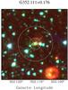 |
Fig. 2 Spitzer/IRAC 3-color image (with 8.0 μm in red, 4.5 μm in green, and 3.6 μm in blue) toward the position of a CH3OH maser (G352.111+0.176, vLSR = −54.8 km s-1), which is marked by the white cross sign (×). Also shown on the image are: (1) the search radius (smaller circle) used to identify the peak “green” value (Rpeak); (2) the search radius (larger circle) used to identify the background value (Rbg); (3) the contour that defines the candidate green source in the image; and (4) the position of the CH3OH maser (×). Note that the cross (×) indicates only the position of the maser, and the size of the cross has no meaning. |
To determine a local background ratio value near the position of the 6.7 GHz maser, we draw an additional aperture with a 30′′ radius centered on the maser position (again, see Fig. 2). We define the local ratio background, Rbg, as the median value of the pixels within the annulus defined by the 10′′ and 30′′ apertures.
With Rpeak and Rbg, we calculate the minimum ratio value, Rcut, required to be included as part of the candidate green source, by taking their average: Rcut = [Rpeak + Rbg] /2. To find candidate green sources, we find all pixels (Npix) with R ≥ Rcut that are contiguous with the peak green value (Rpeak). In this way, we find a candidate green source for each 6.7 GHz maser. The contour in Fig. 2 shows the pixels identified as the candidate green source.
To determine which candidate green sources are bonafide green sources, we require that they meet two more criteria: (1) a minimum number of pixels; and (2) a minimum green value threshold, calculated by taking the average green value of the background-subtracted pixels (Rthresh). To arrive at a value for this threshold, we use a prior known sample of green source/CH3OH maser pairs from Chambers et al. (2011). Using green sources that were identified by eye, Chambers et al. (2011) found that 14 of the masers from C10 were associated with their visually selected sample of green sources. To optimize our algorithm, we use a combination of number of pixels and Rthresh that identifies most or all of the associations found by Chambers et al. (2011), while minimizing the number of spurious associations. We find that a minimum of 9 pixels and Rthresh ≥ 0.2 properly identifies 13 of the 14 (93%) green source/CH3OH maser pairs from Chambers et al. (2011) and finds few spurious detections. This result is shown graphically in Fig. 3. Thus, we use these values to determine our final green source list from the candidate green sources.
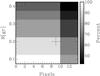 |
Fig. 3 Rgr vs. the number of pixels contained in candidate green sources. To determine the values used as selection criteria in our detection algorithm, we apply different combinations of these values to a known sample of green source/maser pairs to see how many the algorithm recovers. The grayscale shows the percent of known pairs recovered for each set of values. In our algorithm, we use a minimum number of 9 pixels and Rgr ≥ 0.2 as the cutoffs for green sources (marked with a black + in the image). With these values, we recover 13 of 14 (93%) green source/maser pairs. |
To examine the bias in this method, we search for green sources toward random positions. These results are found in Sect. 4.1.1.
3.2. Identification of H2O masers
To identify H2O masers in the Mopra CMZ map, we use the Clumpfind algorithm (Williams et al. 1994). Clumpfind identifies clumps by finding local peaks within a contoured data cube. Contour intervals (used to separate blended features) and lower detection limits are provided by the user, and are typically a multiple of the signal-to-noise ratio (SNR) of the data.
In order to determine an appropriate contour interval and lower limit for our Mopra data, we first analyze the SNR of the input data cube. After masking the line-free channels at each position, we calculate the noise in each spectrum, resulting in the 2d “noise” image shown in Fig. 4. This 2D image clearly shows that the noise in the Mopra H2O data is not uniform throughout the entire cube, which is likely a result of having in different integration times in some regions, as well as varying weather during the observations. Because Clumpfind works best on data with uniform noise, we divide the original data cube by the 2D SNR image, resulting in a data cube containing SNR values. This cube is then used as the input for Clumpfind. We find that, for the SNR data cube, a minimum threshold (i.e., detection limit) of 4 and a contour interval (used to separate blended features) of 4 work best for identifying the H2O masers in the data.
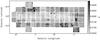 |
Fig. 4 Noise in the spectrum at each position in the Mopra data cube. Because of the uneven noise throughout the data, we divide the original data cube by this 2D image, resulting in a signal-to-noise data cube. The grayscale bar on the right shows the noise temperature in units of K (the conversion to Jy is 12.3 Jy/K). |
In addition to the threshold and contour levels, we also select a minimum number of volume elements (voxels) required for a source to be identified. Based on the Mopra beam size at the frequency of the H2O maser transition (FWHM ~ 144′′ at 22.2 GHz) and the angular size of one pixel (30′′ by 30′′), we require a source to have at least 18 voxels to be included in our final list of masers.
4. Results
4.1. CH3OH masers and green sources
C10 detect 183 CH3OH masers in their survey region (6 °> ℓ > 345°, |b| < 2°), with a 1σ detection limit of 0.07 Jy. Histograms of the maser distribution as a function of ℓ and b can be seen in Fig. 5. The distribution in Galactic latitude shows that the masers have a roughly Gaussian distribution, centered on the Galactic plane. The Galactic longitude distribution displays a peak toward the Galactic center, mostly due to a large number of masers in the Sgr B star forming region. Figure 6 contains a 2D image of the maser distribution, and clearly shows the peak of the maser distribution in Sgr B.
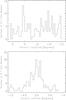 |
Fig. 5 Top: histogram of the distribution of 6.7 GHz masers in Galactic longitude (integrated over all Galactic latitudes). The bin size is 1.5°. The peak of the distribution is largely due to the cluster of 11 masers in Sgr B2. Bottom: histogram of the distribution of 6.7 GHz masers in Galactic latitude (integrated over all Galactic longitudes). The bin size is 0.15°. The masers are distributed around the Galactic equator. |
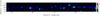 |
Fig. 6 Distribution of the 6.7 GHz CH3OH masers from C10. The pixel size is 0.25°. The bright peak at (ℓ,b) = (0.66, −0.04) is from a cluster of masers in Sgr B2. |
We run the green source detection algorithm (described above) on 175 of the 183 masers in the C10 catalog (8 were excluded because we do not have corresponding IRAC data). We find that 86/175 (49.1 ± 5.3%) of the 6.7 GHz masers are associated with a green source. These green sources range in size from 9 IRAC pixels (the minimum based on our detection method) to 517 IRAC pixels, with a median of 17 IRAC pixels (IRAC pixels are 1.2′′ by 1.2′′). See Fig. 7 for a histogram of the number of pixels in green sources.
A summary of these results can be found in Table B.1, which lists, for each CH3OH maser, the maser name (Col. 1; from C10), the velocity of peak maser emission (Col. 2; from C10), the Galactic longitude, latitude and value for the peak green pixel in each green source candidate, Rpeak (Cols. 3–5), the background green value near each green source candidate, Rbg (Col. 6), the green value used to define the boundary of the green source candidate, Rcut (Col. 7), the average green value for the pixels within the green source candidate, Rthresh (Col. 8), and the number of pixels, Npix, in the green source candidate (Col. 9). The final column in Table B.1 contains a flag (“Y” or “N”; Col. 10) to indicate if a green source is associated with a CH3OH maser based on the values in Cols. 3 through 9.
Using these detected sources, we calculate the detection rates for green sources toward 6.7 GHz masers as a function of Galactic longitude and latitude. In Fig. 8, we show that the longitude distribution of detection rates varies between 20% and 86%, with typical errors of ~20%. The distribution shows possible enhancements at ℓ ~ −2° and ℓ ~ −8°, and a depressed rate at ℓ ~ −5°. The distribution of green source detection rates as a function of Galactic latitude, shown in Fig. 8, shows a clear deficit of green sources detected near the midplane (b ~ 0°) of the Galaxy. The central 0.3° has a detection rate of ~35 ± 10%, while the regions with |b| > 0.5° have detection rates of >50%, with some bins at 100%.
Because we want to compare Galactic center candidate sources to Galactic disk sources, we need a method to estimate the distances to the sources. To determine if the green sources are foreground or Galactic center sources, we use their Galactic coordinates with respect to the Galactic plane and their corresponding maser velocities. First, we use the Galactic coordinates of the sources to separate our sources into GC sources and non-GC sources. To cover the CMZ, and to match the scale height of young stellar objects in the Galactic center region (Yusef-Zadeh et al. 2009), we define the GC region to be |ℓ| < 1.3°, |b| < 10′. Using these criteria for distance, we find that 8/23 GC CH3OH masers (34.8 ± 12.3%) are associated with green sources, and 78/152 (51.3 ± 5.8%) non-GC CH3OH masers are associated with green sources. These association rates are listed in Table 1, which lists the method of distance estimation in Col. 1, the location of the masers in Col. 2, the number of CH3OH masers at that distance in Col. 3, the number of those masers that are associated with green sources in Col. 4, and the association rate calculated on those numbers in Col. 5. Figure 9 shows the positions of the CH3OH masers, their assigned locations (based on their Galactic coordinates), and the velocities of the peak maser emission.
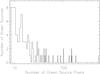 |
Fig. 7 Histogram of the number of pixels in the green sources associated with 6.7 GHz CH3OH masers. The sizes (in IRAC pixels) range from 9 (the minimum based on our detection method) to 517, with a median of 17. |
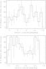 |
Fig. 8 Top: histogram of the percentage of 6.7 GHz masers associated with
green sources as a function of Galactic longitude. Bottom:
histogram of the percentage of 6.7 GHz masers associated with green sources as a
function of Galactic latiitude. The bin size is 0.15°. Errors for the detection rates in
both histograms are calculated using |

Association rates of CH3OH masers with green sources.
Next, we use the distance estimates made by C10, who based their estimates on the velocities of the CH3OH masers and a model of circular Galactic rotation (and allowing for small deviations; see C10 for more details). In short, some maser velocities are consistent with Galactic rotation models, and are placed outside the GC region. Other masers have velocities consistent with a location within the 3 kpc arms, and are assigned that location. Those masers that fit neither of these categories, and have |ℓ| < 1.3° (with no restriction in Galactic latitude) are placed at the distance of the GC. Using these criteria for distance, we find that 13/27 GC CH3OH masers (48.1 ± 13.3%) are associated with green sources, and 73/148 (49.3 ± 5.8%) non-GC CH3OH masers are associated with green sources.
Finally, we also look at the subset of sources that meet the position (by Galactic coordinates) and velocity criteria described above. These masers all have positions with |ℓ| < 1.3°, |b| < 10′, and velocities that are inconsistent with both standard Galactic rotation and placement in the 3 kpc arms. Using these criteria for distance, we find that 4/17 GC CH3OH masers (23.5 ± 11.8%) are associated with green sources, and 82/158 (51.9 ± 5.7%) non-GC CH3OH masers are associated with green sources.
4.1.1. Random test
To determine if the association rates are true associations of green sources with 6.7 GHz masers or simply chance alignments of the two star formation indicators, we placed test masers in the survey longitude and latitude ranges and searched for green sources using the same method described above. Because the C10 CH3OH masers are roughly evenly distributed in longitude, our test masers have a uniform distribution in longitude. To match the latitude distribution of masers seen in Fig. 5, we fit a Gaussian to the distribution and used its parameters to generate the Galactic latitude distribution of test masers. We placed 175 test masers in the survey region, to match the number of masers in the C10 catalog. To increase the statistics, we ran the test a total of ten times. We find a test maser-green source association rate of 1.3 ± 0.3% for our total sample of 1750 test masers. Thus, we consider the chances of our detection rates being contaminated by random chance associations to be small.
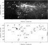 |
Fig. 9 Top: Spitzer/IRAC 8 μm image of the Galactic center region showing 6.7 GHz CH3OH masers. Crosses (+) indicate the positions of 6.7 GHz CH3OH masers placed in the Galactic center region based on position. The × symbols indicate the positions of 6.7 GHz CH3OH masers placed in the Galactic center region based on velocity. The asterisks (*) indicate the positions of 6.7 GHz CH3OH masers placed in the Galactic center region based on both distance criteria. The squares show the locations of the masers thought to reside in the disk. Sources that are circled are associated with an enhanced 4.5 μm emission source. Each maser is labelled with the velocity (in km s-1) of the peak maser emission. Bottom: same as the top figure, but with a blank background instead of the 8 μm image. |
4.2. H2O masers
Using the Clumpfind detection algorithm as described in Sect. 3.2, we find a total of 37 H2O masers. These masers are listed in Table 2, which contains the identification numbers (Col. 1), the Galactic coordinates of the masers (Cols. 2 and 3), the velocity of peak emission for each maser (Col. 4), the peak intensities of the masers (Col. 5), and the number of voxels in the source (Col. 6). The peaks range from 52 mK to 9.54 K, with an average of 1.02 K and a median of 160 mK, and the velocities range from −208.5 to 129.4 km s-1. Spectra of all 37 detections can be seen in Fig. A.1. The distribution of the water masers as a function of Galactic longitude and latitude can be seen in Fig. 10. In Fig. 11, the positions of the water masers are overplotted on an image of the Galactic center region, along with the velocities of the peak maser emission. Some masers share the same positions but have different velocities. These likely comprise a cluster of masers, but higher angular resolution observations are needed to determine their positions more precisely.
H2O masers in the survey region.
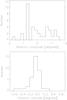 |
Fig. 10 Distribution of the Mopra H2O masers as a function of Galactic longitude (top) and latitude (bottom). The peak of the longitude distribution is due to the 9 masers associated with Sgr B. |
The most notable feature in these distributions is the peak of H2O masers at ℓ ~ 0.6°, which can be attributed to the H2O maser emission from Sgr B2. We detect a total of 9 H2O masers toward Sgr B, including the three strongest emission features in the survey. Figure 12 shows a spectrum toward Sgr B that indicates the velocities of these 9 masers, which are spread from ~0 to ~140 km s-1.
4.2.1. Association of CH3O masers and H2O masers
To associate H2O and CH3OH masers, we first combine three H2O maser lists-the list of masers we found in our Mopra CMZ survey, the list of masers identified by Caswell et al. (2011), and the list of masers from HOPS (Walsh et al. 2011). In order to see the complete results for each list, we do not remove H2O masers that were identified in multiple lists.
We search for H2O masers that are within one beam of CH3OH masers. This separation corresponds to either 144′′ or 10′′, depending on the telescope used to identify the H2O masers. Figure 13 shows the positions of H2O and CH3OH masers overlaid on an image of the GC region. The positions of the H2O masers identified using Mopra are marked by circles that match the Mopra beam size, while the H2O masers identified with ATCA are marked with a × symbol. Crosses (“+”) mark the positions of CH3OH masers (the sizes of the × symbols and crosses have no physical meaning). We consider a H2O and CH3OH maser to be associated when the position of the CH3OH maser falls within the appropriate H2O maser beam.
 |
Fig. 11 Top: Spitzer/IRAC 8 μm image of the Galactic center region. Crosses (+) indicate the positions of the H2O masers identified in the Mopra survey. Each maser is labelled with the velocity (in km s-1) of the peak maser emission. Bottom: same as the top figure, but with a blank background instead of the 8 μm image. |
Because of the relatively large Mopra beam at 22.23 GHz (144′′), and since most of the H2O masers on our combined list are identified using this facility, we are unable to definitively state that a given H2O maser arises from the same location as its “associated” CH3OH maser. Indeed, the “associated” masers may arise from different young stars within the same star formation region, or could be aligned by chance. Nevertheless, we make associations between these two types of masers as described above, and hope for future high angular resolution observations to make a more definitive association.
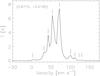 |
Fig. 12 Mopra H2O maser spectrum toward Sgr B. The position of the spectrum (in ℓ,b) is printed at the top of the plot. The vertical lines indicate the velocities of masers identified by the Clumpfind routine. The velocities of the masers identified are 2.2, 31.3, 42.2, 53.1, 71.3, 100.4, 111.3, 122.2, and 129.4 km s-1. The conversion to Jy is 12.3 Jy/K. |
The results of our H2O-CH3OH maser association method, including the velocity information of the masers, are listed in Table B.2. Columns 1−3 of the table list the CH3OH maser name (from C10), and the lower and upper velocity limits of the CH3OH maser emission (from C10). In Cols. 4−7, we list the properties of the H2O masers that are associated with the CH3OH masers-their Galactic coordinates, the velocities of their peak emission, and the catalog from which the maser was identified. Column 8 lists the angular separation between the associated CH3OH and H2O masers. Column 9 indicates if the CH3OH maser is associated with a green source. If a CH3OH maser is associated with multiple H2O masers, then the CH3OH maser information is printed only once, and a line for each of the H2O masers is printed.
Because 22 GHz H2O masers are found in shocks and outflows, their velocities may not match the velocities of the radiatively excited 6.7 GHz CH3OH masers. Therefore, we do not use the velocities of the masers as association criteria. The velocities of both types of masers are listed in Table B.2.
Some of the H2O masers are associated with more than one CH3OH maser. Without higher angular resolution, we are unable to tell if the masers are exactly coincident or are just nearby to one another. Nevertheless, we include these associations, along with whether or not the CH3OH maser is coincident with a green source, to examine the star formation in the CMZ, as well as to determine candidates for potential follow-up observations at higher angular resolution.
Of the 175 CH3OH masers in the C10 catalog, 154 fall within the combined regions of our Mopra CMZ survey, the Caswell et al. (2011) observations, and HOPS. Of these 154, 62 are associated with H2O masers, while 92 are not. The list of these 62 CH3OH masers can be found in the first column of Table B.2.
The combination of our Mopra CMZ survey, the Caswell et al. (2011) observations, and HOPS, yields a total of 177 H2O masers, 63 of which are associated with CH3OH masers. Note that the same H2O masers may be identified by more than one survey, and are thus counted more than once. All of these H2O masers, along with their names or identification numbers, can be found in Table B.2. Because H2O masers can be associated with more than one CH3OH maser, some of the H2O masers are listed more than once in this table. For completeness, we also include Table B.3, which lists CH3OH masers that are not associated with H2O masers. The first three columns of Table B.3 contain the name and Galactic coordinates of the CH3OH masers (from C10), Cols. 4 and 5 contain the minimum and maximum velocities of the maser features (from C10), the peak intensity of the maser emission is in Col. 6, and the last column contains a flag indicating if the CH3OH maser is associated with a green source. In addition, we list H2O masers that are not associated with CH3OH masers in Table B.4. The columns in this table are: (1) the name or number of the H2O maser; (2) the Galactic longitude of the maser; (3) the Galactic latitude of the maser; (4) the velocity of the peak emission from the maser; and (5) the peak emission of the maser. It is interesting to note that each of the 8 strongest H2O masers from our Mopra survey (numbers 1 through 8 in Table 2) are associated with CH3OH masers, and are thus not included in Table B.4.
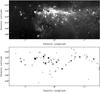 |
Fig. 13 Top: Spitzer/IRAC 8 μm image of the Galactic center region showing both CH3OH and H2O masers. Circles indicate the positions of the H2O masers identified in the Mopra survey and the masers identified by Walsh et al. (2011). The size of the circle represents the FWHM of the Mopra beam at 22 GHz. The × symbols indicate the positions of H2O masers identified by Caswell et al. (2011), and crosses (+) show the position of CH3OH masers (the size of the × symbols and the crosses have no physical meaning). We consider a CH3OH maser to be associated with a H2O maser when it falls within the H2O maser beam. For details on these associations, including their velocity information, see Table B.2. Bottom: same as the top figure, but with a blank background instead of the 8 μm image. |
5. Discussion
5.1. CH3OH/green source association rate as a function of Galactic longitude
To search for trends in the association rate of 6.7 GHz masers and 4.5 μm emission, we binned the sources (and association rates) by Galactic Longitude. The results are shown in Fig. 8. The association rate varies from bin to bin (from 20 ± 14% to 85 ± 25%), but we find no strong trend with Galactic longitude. There appears to a decrement of associations at ℓ ~ −5°, and enhancements of associations at ℓ ~ −2°and −8°. Because of the large error bars and the large bin-to-bin variations, we consider the likely cause of these to be the results of small number statistics and binning.
5.2. CH3OH/green source association rate as a function of Galactic latitude
We find that CH3OH masers near the Galactic midplane(|b| < 10′) are less likely (34.8 ± 6.4%) to be associated with green sources than those above or below it (62.9 ± 8.4%). While this could be a real effect, and masers outside the midplane could simply have higher association rates with 4.5 μm sources than those in the midplane, we find it much more likely to be an optical depth effect of having two star formation tracers at very different wavelengths/frequencies.
The Galactic plane is optically thin at 6.7 GHz, making it possible to detect 6.7 GHz CH3OH masers throughout the Galaxy, including the far side of the Galactic plane. This is not the case, however, for 4.5 μm emission. At this much shorter wavelength, extinction plays a much larger role (see, e.g., Pandey & Mahra 1987), preventing the detection of green sources on the far side of the Galaxy (behind, e.g., the molecular clouds on the near side of the Galaxy). Because the extinction is higher in the Galactic plane, we are likely to have a cleaner line of sight to 6.7 GHz masers that reside above or below the Galactic plane. Thus, we find a lower association rate of 4.5 μm emission with 6.7 GHz CH3OH masers for sources that are in the midplane of the Galaxy (l < 10′) than those above or below it.
5.3. Comparing the Galactic center with the Galactic disk
To see how star formation in the Galactic center region may differ from that of the disk, we compare the 6.7 GHz CH3OH association rate with enhanced 4.5 μm emission. As described in Sect. 4.1, we make three different distance esimates based on the positions of the masers, the velocities of the masers, and the combination of these two criteria.
Using Galactic coordinates alone(|ℓ| < 1.3°, |b| < 10′) to estimate the distances to the CH3OH masers, and assuming that all masers that fit the distance criteria are indeed in the GC (and not the foreground), we find that 34.8 ± 12.3% are associated with green sources in the GC, and that 51.3 ± 5.8% of disk sources are associated with green sources. The association rate for the disk includes all Galactic latitudes. Because the GC is in the Galactic midplane, however, we should compare the GC association rate to the association rate in the rest of the midplane (6°> ℓ > 345°), excluding the GC longitudes(|ℓ| < 1.3°). When we do this, we find that the disk midplane association rate is 34.9 ± 7.4%, very close to the association rate for the GC. Thus, we find no differences between the two regions using position alone as a distance indicator.
When we use only the source velocity to estimate the locations of the masers, we find nearly identical association rates between the CH3OH masers and the enhanced 4.5 μm emission sources in the GC (48.1 ± 13.3%) and the disk (49.3 ± 5.8%). Because the positions of the masers are not considered in this distance estimate, no adjustment for the midplane is necessary. The similar association rates again point to no significant difference between the GC and disk regions.
Using both positional and velocity criteria to place sources at the distance of the Galactic center, we find a detection rate (23.5 ± 11.8%) that is lower than that of all other midplane sources (34.9 ± 7.4%). While the association rate in the GC is lower using both distance criteria, the large error bars keep this from being a significant result. When we look at the sources placed in the GC region by only one of the two indicators (position or velocity), we find that they have high association rates, 66.7 ± 33.3% for those sources whose positions match the GC, and 90.0 ± 30.0% for those whose velocities match the GC. Figure 14 shows a diagram with these association rates. These elevated rates could simply be a result of small number statistics, since when taking into account their error bars, they are consistent with the disk association rate, especially at larger Galactic latitudes. Nevertheless, this difference remains intriguing.
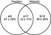 |
Fig. 14 Diagram showing green source detection rates based on two different distance estimates. Sources placed in the Galactic center based on position all have |ℓ| < 1.3° and |b| < 10′. Distance estimates based on velocity are taken from C10. For comparison, the green source detection rates for masers that are not at the distance of the Galactic center (based on position or velocity) is 48.6 ± 5.9% (69/142). |
As described in Sect. 4.2.1, the combination of our Mopra CMZ survey, the Caswell et al. (2011) observations, and HOPS, yields a total of 177 H2O masers within the region 30 °> ℓ > 290°, |b| < 0.5°. This covers the entire CMZ as well as a large part of the Galactic disk outside of the CMZ. Using this list, we can compare the association rates of CH3OH masers with H2O masers in the CMZ to those outside the CMZ, as determined by their positions. We find that of the 23 CH3OH masers in the CMZ, 15 are spatially associated with H2O masers (65 ± 17%). Outside of the CMZ, we find that 47 of the 131 CH3OH masers (36 ± 5%) are associated with H2O masers. Thus, there appears to be a significant difference between the correlation of CH3OH and H2O masers in these regions.
It is important to note that H2O masers are also found toward AGB stars. These H2O masers tend to be less luminous than those found toward high-mass star forming regions (Palagi et al. 1993; Caswell et al. 2011). Indeed, in the Caswell et al. (2011) ATCA 0.5 deg2 H2O maser survey of the Galactic center, they found that only 3 of their 27 detected masers could be definitely attributed to AGB stars. Using this detection rate, ~4 of the 37 H2O masers detected in our Mopra survey and ~13 of 113 H2O masers in HOPS, may be associated with evolved AGB stars rather than sites of star formation. The H2O masers associated with CH3OH masers or green sources are very unlikely to also be associated with AGB stars. Thus, the effect of the small number of AGB H2O masers in our sample is negligible.
The fact that we find significantly fewer H2O masers toward the CH3OH masers outside the CMZ is intriguing, and may be related to a different timescale of star formation inside the CMZ when compared to the Galactic disk. While still somewhat speculative, some recent work (Ellingsen et al. 2007; Breen et al. 2010) has proposed an evolutionary sequence of CH3OH masers in which Class I CH3OH masers, generated by protostellar outflows, are formed before radiatively excited Class II CH3OH masers (e.g., the 6.7 GHz CH3OH maser). In addition, some observations have suggested that the 22 GHz H2O maser also arises in an early phase of star formation and overlaps with the Class I CH3OH masers, in particular toward green sources (e.g., Chambers et al. 2009). Thus, if we assume that the 22 GHz H2O masers arise at an earlier evolutionary state than the 6.7 GHz CH3OH masers, then perhaps the much higher correlation rate of the two masers in the GC (65% vs. 36%) corresponds to a longer overlap period of the two stages. This result can be tested using higher-resolution H2O maser data to verify the GC correlations, a larger number of H2O and CH3OH masers in the GC (from more sensitive surveys), as well as large co-spatial surveys of H2O and CH3OH masers in the Galactic plane to better establish the correlation rate in the disk.
5.4. Asymmetry in the H2O maser distribution around the Galactic center
Yusef-Zadeh et al. (2009) found an asymmetry in the distribution of young stellar object (YSO) candidates as probed by 24 μm sources, with a larger number of YSO candidates with ℓ < 0 relative to ℓ > 0. The distribution of Mopra CMZ H2O masers as a function of Galactic longitude (Fig. 10) shows no obvious asymmetry with respect to ℓ = 0, with 19 masers having ℓ > 0 and 18 masers having ℓ < 0. The most striking feature in this distribution of H2O masers is the peak at ~ℓ = 0.7, which is almost entirely due to masers in Sgr B2 (10 of the 11 masers in the bin have coordinates that place them within Sgr B2). If we remove these 10 masers from the distribution, we find that there are 11 H2O masers with ℓ > 0, and 16 with ℓ < 0, consistent with the asymmetry found by Yusef-Zadeh et al. (2009). One explanation for the asymmetry offered by Yusef-Zadeh et al. (2009) was that higher extinction due to dense clouds may be responsible for the asymmetry in the distribution of 24 μm sources. Extinction is not a problem at the frequency of the H2O masers, suggesting that the asymmetry may be a real feature. The larger numbers of both 24 μm sources and H2O masers at ℓ < 0 indicate an enhancement of on-going star formation in this region.
6. Conclusions
We present the results of our study of star formation in the CMZ and how it compares to the Galactic disk. We make our comparison through the correlation of 6.7 GHz CH3OH masers, 22 GHz H2O masers, and green sources. As part of this study, we developed an automated algorithm to identify regions of extended, enhanced 4.5 μm emission toward 6.7 GHz CH3OH masers. This new technique can be a powerful tool to trace regions of star formation provided the column density along the line of sight is not too high. Moreover, we used the Mopra telescope to survey the 22 GHz H2O maser emission in the CMZ, resulting in the detection of 37 individual water masers.
We find that the association rate of CH3OH masers with green sources as a function of Galactic longitude is relatively flat. In Galactic latitude, on the other hand, we find that there is a significant decrease in the association rate along the Galactic midplane, which is likely an infrared extinction effect. Using two different distance estimates, we do not detect any significant difference in the association rates of green sources with CH3OH masers between the Galactic center and the disk. This suggests that once the star formation process has begun, its observational signatures are similar in the GC and the Galactic disk, despite the different physical conditions of the gas in the two regions.
We find that CH3OH masers are much more likely to be associated with a H2O maser if they are located in the Galactic center rather than the Galactic disk, indicating a longer overlap period between these two masers in the GC. Future high angular resolution observations of the newly detected H2O masers are needed to better establish the positions of the H2O masers and test this result.
Online material
Appendix A: Mopra H2O spectra
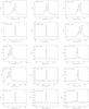 |
Fig. A.1 Spectra of H2O masers 1–15 detected in the survey region. The positions of the peak emission are printed on the spectra, and the numbers in the top-right of each plot correspond to the numbers in Table 2. The vertical line in each spectrum indicates the velocity of that maser. |
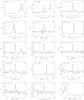 |
Fig. A.1 continued. |
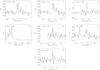 |
Fig. A.1 continued. |
Appendix B: Supplementary tables
Association of green sources with CH3OH masers.
Association of H2O masers with CH3OH masers.
CH3OH masers not associated with H2O masers.
H2O masers not associated with CH3OH masers.
Acknowledgments
We are grateful to the referee, Andrew Walsh, whose comments and suggestions greatly improved the paper. This research is carried out within the Collaborative Research Centre 956, sub-project A4, funded by the Deutsche Forschungsgemeinschaft (DFG). This work is partially supported by grant AST-0807400 from the NSF. The National Radio Astronomy Observatory is a facility of the National Science Foundation operated under cooperative agreement by Associated Universities, Inc. The Australia Telescope Compact Array, Parkes radio telescope, and Mopra radio telescope are part of the Australia Telescope National Facility which is funded by the Commonwealth of Australia for operation as a National Facility managed by CSIRO.
References
- Ao, Y., Henkel, C., Menten, K. M., et al. 2013, A&A, 550, A135 [NASA ADS] [CrossRef] [EDP Sciences] [Google Scholar]
- Arendt, R. G., Stolovy, S. R., Ramírez, S. V., et al. 2008, ApJ, 682, 384 [NASA ADS] [CrossRef] [Google Scholar]
- Benjamin, R. A., Churchwell, E., Babler, B. L., et al. 2003, PASP, 115, 953 [NASA ADS] [CrossRef] [Google Scholar]
- Breen, S. L., Ellingsen, S. P., Caswell, J. L., & Lewis, B. E. 2010, MNRAS, 401, 2219 [NASA ADS] [CrossRef] [Google Scholar]
- Caswell, J. L. 1997, MNRAS, 289, 203 [NASA ADS] [CrossRef] [Google Scholar]
- Caswell, J. L., Fuller, G. A., Green, J. A., et al. 2010, MNRAS, 404, 1029 [NASA ADS] [CrossRef] [Google Scholar]
- Caswell, J. L., Breen, S. L., & Ellingsen, S. P. 2011, MNRAS, 410, 1283 [NASA ADS] [CrossRef] [Google Scholar]
- Chambers, E. T., Jackson, J. M., Rathborne, J. M., & Simon, R. 2009, ApJS, 181, 360 [NASA ADS] [CrossRef] [Google Scholar]
- Chambers, E. T., Yusef-Zadeh, F., & Roberts, D. 2011, ApJ, 733, 42 [NASA ADS] [CrossRef] [Google Scholar]
- Chen, X., Ellingsen, S. P., & Shen, Z.-Q. 2009, MNRAS, 396, 1603 [NASA ADS] [CrossRef] [Google Scholar]
- Claussen, M. J., Marvel, K. B., Wootten, A., & Wilking, B. A. 1998, ApJ, 507, L79 [NASA ADS] [CrossRef] [Google Scholar]
- Cox, P., & Laureijs, R. 1989, The Center of the Galaxy, held in Los Angeles (Dordrecht: Kluwer Academic Publishers), Proc. IAU Symp., 136, 121 [NASA ADS] [Google Scholar]
- Cragg, D. M., Johns, K. P., Godfrey, P. D., & Brown, R. D. 1992, MNRAS, 259, 203 [NASA ADS] [CrossRef] [Google Scholar]
- Cyganowski, C. J., Whitney, B. A., Holden, E., et al. 2008, AJ, 136, 2391 [NASA ADS] [CrossRef] [Google Scholar]
- Cyganowski, C. J., Brogan, C. L., Hunter, T. R., & Churchwell, E. 2009, ApJ, 702, 1615 [NASA ADS] [CrossRef] [Google Scholar]
- De Buizer, J. M., & Vacca, W. D. 2010, AJ, 140, 196 [NASA ADS] [CrossRef] [Google Scholar]
- Elitzur, M., Hollenbach, D. J., & McKee, C. F. 1989, ApJ, 346, 983 [NASA ADS] [CrossRef] [Google Scholar]
- Ellingsen, S. P. 2005, MNRAS, 359, 1498 [NASA ADS] [CrossRef] [Google Scholar]
- Ellingsen, S. P., Voronkov, M. A., Cragg, D. M., et al. 2007, IAU Symp., 242, 213 [NASA ADS] [Google Scholar]
- Fazio, G. G., Hora, J. L., Allen, L. E., et al. 2004, ApJS, 154, 10 [NASA ADS] [CrossRef] [Google Scholar]
- Ferrière, K., Gillard, W., & Jean, P. 2007, A&A, 467, 611 [NASA ADS] [CrossRef] [EDP Sciences] [Google Scholar]
- Furuya, R. S., Kitamura, Y., Wootten, H. A., Claussen, M. J., & Kawabe, R. 2001, ApJ, 559, L143 [NASA ADS] [CrossRef] [Google Scholar]
- Genzel, R., Downes, D., Moran, J. M., et al. 1978, A&A, 66, 13 [NASA ADS] [Google Scholar]
- Gwinn, C. R. 1994, ApJ, 429, 241 [NASA ADS] [CrossRef] [Google Scholar]
- Hollenbach, D., Elitzur, M., & McKee, C. F. 2013, ApJ, 773, 70 [NASA ADS] [CrossRef] [Google Scholar]
- Houghton, S., & Whiteoak, J. B. 1995, MNRAS, 273, 1033 [NASA ADS] [Google Scholar]
- Huettemeister, S., Dahmen, G., Mauersberger, R., et al. 1998, A&A, 334, 646 [Google Scholar]
- Immer, K., Menten, K. M., Schuller, F., & Lis, D. C. 2012, A&A, 548, A120 [NASA ADS] [CrossRef] [EDP Sciences] [Google Scholar]
- Jones, P. A., Burton, M. G., Tothill, N. F. H., & Cunningham, M. R. 2011, MNRAS, 411, 2293 [NASA ADS] [CrossRef] [Google Scholar]
- Jones, P. A., Burton, M. G., Cunningham, M. R., et al. 2012, MNRAS, 419, 2961 [NASA ADS] [CrossRef] [Google Scholar]
- Jones, P. A., Burton, M. G., Cunningham, M. R., Tothill, N. F. H., & Walsh, A. J. 2013, MNRAS, 433, 221 [NASA ADS] [CrossRef] [Google Scholar]
- Kennicutt, R. C., Jr. 1998, ARA&A, 36, 189 [Google Scholar]
- Longmore, S. N., Rathborne, J., Bastian, N., et al. 2012, ApJ, 746, 117 [NASA ADS] [CrossRef] [Google Scholar]
- Marston, A. P., Reach, W. T., Noriega-Crespo, A., et al. 2004, ApJS, 154, 333 [NASA ADS] [CrossRef] [Google Scholar]
- Martín-Pintado, J., de Vicente, P., Rodríguez-Fernández, N. J., Fuente, A., & Planesas, P. 2000, A&A, 356, L5 [NASA ADS] [Google Scholar]
- Menten, K. M. 1991, ApJ, 380, L75 [NASA ADS] [CrossRef] [Google Scholar]
- Mills, E. A. C., & Morris, M. R. 2013, ApJ, 772, 105 [Google Scholar]
- Pandey, A. K., & Mahra, H. S. 1987, MNRAS, 226, 635 [NASA ADS] [Google Scholar]
- Minier, V., Ellingsen, S. P., Norris, R. P., & Booth, R. S. 2003, A&A, 403, 1095 [NASA ADS] [CrossRef] [EDP Sciences] [Google Scholar]
- Molinari, S., Bally, J., Noriega-Crespo, A., et al. 2011, ApJ, 735, L33 [NASA ADS] [CrossRef] [Google Scholar]
- Morris, M., & Serabyn, E. 1996, ARA&A, 34, 645 [NASA ADS] [CrossRef] [Google Scholar]
- Noriega-Crespo, A., Morris, P., Marleau, F. R., et al. 2004, ApJS, 154, 352 [NASA ADS] [CrossRef] [Google Scholar]
- Norman, C., & Silk, J. 1979, ApJ, 228, 197 [NASA ADS] [CrossRef] [Google Scholar]
- Odenwald, S. F., & Fazio, G. G. 1984, ApJ, 283, 601 [NASA ADS] [CrossRef] [Google Scholar]
- Oka, T., Geballe, T. R., Goto, M., Usuda, T., & McCall, B. J. 2005, ApJ, 632, 882 [NASA ADS] [CrossRef] [Google Scholar]
- Palagi, F., Cesaroni, R., Comoretto, G., Felli, M., & Natale, V. 1993, A&AS, 101, 153 [NASA ADS] [Google Scholar]
- Pierce-Price, D., Richer, J. S., Greaves, J. S., et al. 2000, ApJ, 545, L121 [Google Scholar]
- Ramírez, S. V., Arendt, R. G., Sellgren, K., et al. 2008, ApJS, 175, 147 [NASA ADS] [CrossRef] [Google Scholar]
- Rathborne, J. M., Jackson, J. M., Chambers, E. T., Simon, R., Shipman, R., & Frieswijk, W. 2005, ApJ, 630, L181 [NASA ADS] [CrossRef] [Google Scholar]
- Rathborne, J. M., Jackson, J. M., & Simon, R. 2006, ApJ, 641, 389 [NASA ADS] [CrossRef] [Google Scholar]
- Reid, M. J., Menten, K. M., Zheng, X. W., et al. 2009, ApJ, 700, 137 [NASA ADS] [CrossRef] [Google Scholar]
- Riquelme, D., Bronfman, L., Mauersberger, R., May, J., & Wilson, T. L. 2010, A&A, 523, A45 [NASA ADS] [CrossRef] [EDP Sciences] [Google Scholar]
- Stolovy, S., Ramirez, S., Arendt, R. G., et al. 2006, J. Phys. Conf. Ser., 54, 176 [NASA ADS] [CrossRef] [Google Scholar]
- Urquhart, J. S., Hoare, M. G., Purcell, C. R., et al. 2010, PASA, 27, 321 [NASA ADS] [CrossRef] [Google Scholar]
- Walsh, A. J., Bertoldi, F., Burton, M. G., & Nikola, T. 2001, MNRAS, 326, 36 [NASA ADS] [CrossRef] [Google Scholar]
- Walsh, A. J., Breen, S. L., Britton, T., et al. 2011, MNRAS, 416, 1764 [NASA ADS] [CrossRef] [Google Scholar]
- Williams, J. P., de Geus, E. J., & Blitz, L. 1994, ApJ, 428, 693 [NASA ADS] [CrossRef] [Google Scholar]
- Yusef-Zadeh, F., Arendt, R. G., Heinke, C. O., et al. 2007, IAU Symp., 242, 366 [NASA ADS] [Google Scholar]
- Yusef-Zadeh, F., Hewitt, J. W., Arendt, R. G., et al. 2009, ApJ, 702, 178 [NASA ADS] [CrossRef] [Google Scholar]
- Yusef-Zadeh, F., Cotton, W., Viti, S., Wardle, M., & Royster, M. 2013a, ApJ, 764, L19 [NASA ADS] [CrossRef] [Google Scholar]
- Yusef-Zadeh, F., Wardle, M., Lis, D., et al. 2013b, J. Phys. Chem. A, 117, 9404 [CrossRef] [Google Scholar]
All Tables
All Figures
|
Fig. 1 Spitzer/IRAC 3-color image (with 8.0 μm in red, 4.5 μm in green, and 3.6 μm in blue) of the Central Molecular Zone. Some of the more prominent Galactic center features are labelled. Sgr A∗ is centered on the nuclear cluster. |
| In the text | |
|
Fig. 2 Spitzer/IRAC 3-color image (with 8.0 μm in red, 4.5 μm in green, and 3.6 μm in blue) toward the position of a CH3OH maser (G352.111+0.176, vLSR = −54.8 km s-1), which is marked by the white cross sign (×). Also shown on the image are: (1) the search radius (smaller circle) used to identify the peak “green” value (Rpeak); (2) the search radius (larger circle) used to identify the background value (Rbg); (3) the contour that defines the candidate green source in the image; and (4) the position of the CH3OH maser (×). Note that the cross (×) indicates only the position of the maser, and the size of the cross has no meaning. |
| In the text | |
|
Fig. 3 Rgr vs. the number of pixels contained in candidate green sources. To determine the values used as selection criteria in our detection algorithm, we apply different combinations of these values to a known sample of green source/maser pairs to see how many the algorithm recovers. The grayscale shows the percent of known pairs recovered for each set of values. In our algorithm, we use a minimum number of 9 pixels and Rgr ≥ 0.2 as the cutoffs for green sources (marked with a black + in the image). With these values, we recover 13 of 14 (93%) green source/maser pairs. |
| In the text | |
|
Fig. 4 Noise in the spectrum at each position in the Mopra data cube. Because of the uneven noise throughout the data, we divide the original data cube by this 2D image, resulting in a signal-to-noise data cube. The grayscale bar on the right shows the noise temperature in units of K (the conversion to Jy is 12.3 Jy/K). |
| In the text | |
|
Fig. 5 Top: histogram of the distribution of 6.7 GHz masers in Galactic longitude (integrated over all Galactic latitudes). The bin size is 1.5°. The peak of the distribution is largely due to the cluster of 11 masers in Sgr B2. Bottom: histogram of the distribution of 6.7 GHz masers in Galactic latitude (integrated over all Galactic longitudes). The bin size is 0.15°. The masers are distributed around the Galactic equator. |
| In the text | |
|
Fig. 6 Distribution of the 6.7 GHz CH3OH masers from C10. The pixel size is 0.25°. The bright peak at (ℓ,b) = (0.66, −0.04) is from a cluster of masers in Sgr B2. |
| In the text | |
|
Fig. 7 Histogram of the number of pixels in the green sources associated with 6.7 GHz CH3OH masers. The sizes (in IRAC pixels) range from 9 (the minimum based on our detection method) to 517, with a median of 17. |
| In the text | |
|
Fig. 8 Top: histogram of the percentage of 6.7 GHz masers associated with
green sources as a function of Galactic longitude. Bottom:
histogram of the percentage of 6.7 GHz masers associated with green sources as a
function of Galactic latiitude. The bin size is 0.15°. Errors for the detection rates in
both histograms are calculated using |
| In the text | |
|
Fig. 9 Top: Spitzer/IRAC 8 μm image of the Galactic center region showing 6.7 GHz CH3OH masers. Crosses (+) indicate the positions of 6.7 GHz CH3OH masers placed in the Galactic center region based on position. The × symbols indicate the positions of 6.7 GHz CH3OH masers placed in the Galactic center region based on velocity. The asterisks (*) indicate the positions of 6.7 GHz CH3OH masers placed in the Galactic center region based on both distance criteria. The squares show the locations of the masers thought to reside in the disk. Sources that are circled are associated with an enhanced 4.5 μm emission source. Each maser is labelled with the velocity (in km s-1) of the peak maser emission. Bottom: same as the top figure, but with a blank background instead of the 8 μm image. |
| In the text | |
|
Fig. 10 Distribution of the Mopra H2O masers as a function of Galactic longitude (top) and latitude (bottom). The peak of the longitude distribution is due to the 9 masers associated with Sgr B. |
| In the text | |
|
Fig. 11 Top: Spitzer/IRAC 8 μm image of the Galactic center region. Crosses (+) indicate the positions of the H2O masers identified in the Mopra survey. Each maser is labelled with the velocity (in km s-1) of the peak maser emission. Bottom: same as the top figure, but with a blank background instead of the 8 μm image. |
| In the text | |
|
Fig. 12 Mopra H2O maser spectrum toward Sgr B. The position of the spectrum (in ℓ,b) is printed at the top of the plot. The vertical lines indicate the velocities of masers identified by the Clumpfind routine. The velocities of the masers identified are 2.2, 31.3, 42.2, 53.1, 71.3, 100.4, 111.3, 122.2, and 129.4 km s-1. The conversion to Jy is 12.3 Jy/K. |
| In the text | |
|
Fig. 13 Top: Spitzer/IRAC 8 μm image of the Galactic center region showing both CH3OH and H2O masers. Circles indicate the positions of the H2O masers identified in the Mopra survey and the masers identified by Walsh et al. (2011). The size of the circle represents the FWHM of the Mopra beam at 22 GHz. The × symbols indicate the positions of H2O masers identified by Caswell et al. (2011), and crosses (+) show the position of CH3OH masers (the size of the × symbols and the crosses have no physical meaning). We consider a CH3OH maser to be associated with a H2O maser when it falls within the H2O maser beam. For details on these associations, including their velocity information, see Table B.2. Bottom: same as the top figure, but with a blank background instead of the 8 μm image. |
| In the text | |
|
Fig. 14 Diagram showing green source detection rates based on two different distance estimates. Sources placed in the Galactic center based on position all have |ℓ| < 1.3° and |b| < 10′. Distance estimates based on velocity are taken from C10. For comparison, the green source detection rates for masers that are not at the distance of the Galactic center (based on position or velocity) is 48.6 ± 5.9% (69/142). |
| In the text | |
|
Fig. A.1 Spectra of H2O masers 1–15 detected in the survey region. The positions of the peak emission are printed on the spectra, and the numbers in the top-right of each plot correspond to the numbers in Table 2. The vertical line in each spectrum indicates the velocity of that maser. |
| In the text | |
|
Fig. A.1 continued. |
| In the text | |
|
Fig. A.1 continued. |
| In the text | |
Current usage metrics show cumulative count of Article Views (full-text article views including HTML views, PDF and ePub downloads, according to the available data) and Abstracts Views on Vision4Press platform.
Data correspond to usage on the plateform after 2015. The current usage metrics is available 48-96 hours after online publication and is updated daily on week days.
Initial download of the metrics may take a while.