| Issue |
A&A
Volume 563, March 2014
|
|
|---|---|---|
| Article Number | A105 | |
| Number of page(s) | 17 | |
| Section | Cosmology (including clusters of galaxies) | |
| DOI | https://doi.org/10.1051/0004-6361/201322372 | |
| Published online | 17 March 2014 | |
Joint Planck and WMAP CMB map reconstruction⋆
1 Laboratoire AIM, UMR CEA-CNRS-Paris 7, Irfu, SAp/SEDI, Service d’Astrophysique, CEA Saclay, 91191 Gif-Sur-Yvette Cedex, France
e-mail: This email address is being protected from spambots. You need JavaScript enabled to view it.
2 Laboratoire d’astrophysique, École Polytechnique Fédérale de Lausanne (EPFL), Observatoire de Sauverny, 1290 Versoix, Switzerland
Received: 26 July 2013
Accepted: 23 January 2014
Abstract
We present a novel estimate of the cosmological microwave background (CMB) map by combining the two latest full-sky microwave surveys: WMAP nine-year and Planck PR1. The joint processing benefits from a recently introduced component separation method coined“local-generalized morphological component analysis” (LGMCA) and based on the sparse distribution of the foregrounds in the wavelet domain. The proposed estimation procedure takes advantage of the IRIS 100 μm as an extra observation on the galactic center for enhanced dust removal. We show that this new CMB map presents several interesting aspects: i) it is a full sky map without using any inpainting or interpolating method; ii) foreground contamination is very low; iii) the Galactic center is very clean with especially low dust contamination as measured by the cross-correlation between the estimated CMB map and the IRIS 100 μm map; and iv) it is free of thermal SZ contamination.
Key words: cosmic background radiation / methods: data analysis / methods: statistical
Appendix is available in electronic form at http://www.aanda.org
© ESO, 2014
1. Introduction
The cosmic microwave background (CMB) is a snapshot of the state of the Universe at the time of recombination. It provides information about the primordial Universe and its evolution to the current state. Our current understanding of our Universe is heavily based on measurements of the CMB radiation. The statistical properties of CMB fluctuations depend on the primordial perturbations from which they arose, as well as on the subsequent evolution of the Universe as a whole. For cosmological models in which initial perturbations are Gaussian, the information carried by CMB anisotropies can be completely characterized by their angular power spectrum which depends on a few cosmological parameters. This makes the precise measurement of the CMB power spectrum, a gold mine for understanding and describing the Universe throughout its history.
Pictures of the CMB maps delivered by the frequency channels of WMAP (Bennett 2013) or Planck (Planck Collaboration XII 2014) are contaminated by the astrophysical foreground emissions from our galaxy and extragalactic sources. The estimation of an accurate full-sky CMB map requires removing these emissions all over the sky (Bouchet & Gispert 1999). Computing a clean estimate of the CMB map on the Galactic center is particularly challenging. In addition, the instrumental noise hinders estimation of the CMB map. In the low-frequency regime (below 100 GHz, i.e., for WMAP or Planck LFI channels), the strongest contamination comes from the Galactic synchrotron and free-free emission (Gold et al. 2011), with the largest contribution on large angular scales. Spinning dust (Planck Collaboration 2011b) is an extra emission that spatially correlates with dust and dominates at low frequencies. At higher frequencies, the dust emissions (Planck Collaboration 2011a) dominate, whereas the synchrotron, free-free emissions, and spinning dust are low.
The estimation of a clean foreground-free CMB map from the frequency channels is performed best by component separation techniques (Leach et al. 2008). The CMB maps made available by the Planck consortium were obtained by using four different component separation methods (Planck Collaboration XII 2014):
-
SEVEM performs template fitting (Fernández-Coboset al. 2012) in two distinct regionson both the 100 and 143 Ghz maps. Precisely, four templates arederived from the difference of two channel maps (30–44),(44–70), (545–353), and (857–545).The final CMB map is thenobtained by combining the two cleaned 100 and 143 Ghz maps.
-
NILC is an ILC-based method that is performed in the wavelet domain (Delabrouille et al. 2009). The standard NILC approach is applied on each wavelet band, and for different regions. Up to 20 regions were used at the finest band. All Planck channels except the 30 GHz are used.
-
SMICA is a component separation method based on second-order statistics in the spherical harmonic domain (Delabrouille et al. 2003). It includes a modeling of the foreground covariance matrix for ℓ < 1500 and then performs ILC for ℓ > 1500. All Planck channel are used.
-
Commander-Ruler, or CR (Eriksen et al. 2008), considers a sky modeling based on four components (CMB, low-frequency emission, CO emission, and thermal dust emission). Model parameters are derived at a 40 arc minute resolution, and the full resolution sky modeling is obtained by interpolating the parameters. Only channels with frequencies ranging from 30 to 353 GHz are used. At the time this study was done, the CR map was not yet available. This is why it is not discussed in this paper.
The SEVEM map is a full-sky map. The SMICA and NILC maps are not full-sky where masked pixels (about 4% for SMICA) are in-painted or interpolated using a diffuse in-painting method. Furthermore, these maps are contaminated by the Sunyaev Zel’Dovich (SZ) effect, which is problematic for CMB/SZ cross studies.
The quality of component separation methods stronglydepends on the number of degrees of freedom (d.o.f.’s) available to clean foreground contaminants. It is limited by the number of observed frequency channels. From this point, estimating a full-sky map with a cleanGalactic center, along with a low SZ contamination, may sound like a dilemma: on the one hand constraining the SZ effect further requires freezing one d.o.f., and on the other hand the estimation of a clean full-sky CMB map requires a copious number of d.o.f.’s to clean the complex emissivity variations of theGalactic center. Fortunately, additional d.o.f.’s can be included by combining several full-sky microwave surveys such as Planck PR1 and WMAP nine-year data.
Contributions
In this paper, we jointly process the WMAP nine-year and Planck PR1 data to recover a single CMB map. For this purpose, we make use of a recently introduced component separation method called LGMCA (local generalized morphological component analysis, Bobin et al. 2013a). Based on the concept of sparsity (Starck et al. 2013), the LGMCA radically departs from the methods used so far to estimate Planck CMB maps, which all rely on second-order statistics. The combination of the Planck and WMAP data yields a CMB map with significant improvements:
-
full-sky map with no interpolated or inpainted pixels(Fig. 7);
-
very clean estimation of theGalactic region with very low foreground-related artifacts (Sects. 3.1, 3.2);
-
low dust contamination for ℓ < 1000 (Sect. 3.4);
-
virtually no SZ contamination (Sect. 3.3).
Section 2 briefly describes the basics LGMCA method and the details of the joint processing of nine-year WMAP and Planck PR1. The map we derived from LGMCA is displayed and compared with the available Planck-only CMB maps in Sect. 3.
2. Sparsity and CMB map reconstruction
The GMCA method is based on blind source separation (BSS; Bobin et al. 2013a). In the framework of BSS, the observed sky is assumed to be a linear combination ofm components so that the M frequency channels verify  (1)where sj stands for the jth component, aij is a scalar that models the contribution of the jth component to channel i, and ni models the instrumental noise. This problem is more conveniently recast in the matrix formulation:
  (2)Currently available CMB maps that were derived from the Planck PR1 data are all based on the minimization of second-order statistics, with the exception of the parameterized Bayesian method C-R (Commander-Ruler). In contrast, the GMCA method (Bobin et al. 2013a) relies on a radically different separation principle: sparsity. That foreground components are sparse in the wavelet domain (i.e., a few wavelet coefficients are enough to represent most of the energy of the component) with different sparsity patterns means sparsity acts as a good separation criterion. Taking the data to the wavelet representation only alters the statistical distribution of the data coefficients without affecting its information content. A wavelet transform tends to capture the informative coherence between pixels while averaging the noise contributions, thus enhancing the structure in the data. This helps distinguish different components that do not share the same sparse distribution in the wavelet domain. In addition, sparsity has the ability to be more sensitive to non-Gaussian processes, which has been shown to improve the foreground separation method. This is especially true in the Galactic center where the rapid variations in the emissivity of components such as dust emissions or compact sources can be well measured by sparsity-based separation criteria.
Having A as the mixing matrix and Φ as a wavelet transform, we assume that each source si can be sparsely represented in Φ; sj = αjΦ, where α is an Ns × T matrix whose rows are αj. The multichannel noiseless data Y can be written as  (3)The GMCA algorithm seeks an unmixing scheme that yields the sparsest sources S. This is made formal by the following optimization problem (written in the Lagrangian form)
  (4)where typically p = 0 (or its relaxed convex version with p = 1) and
  is the Frobenius norm.
The local-GMCA (LGMCA) algorithm (Bobin et al. 2013a) has been introduced as an extensionto GMCA. Precisely, multifrequency instruments generally provide observations with different resolutions. For example, the WMAP frequency channels have a resolution that ranges from 13.2 arcmin for the W band to 52.8 arcmin for the K band. The Planck PR1 data have a resolution that ranges from 5 arcmin at frequency 857 GHz to 33 arcmin at frequency 30 GHz. The linear mixture model assumed so far in LGMCA no longer holds. This problem can be alleviated by degrading the frequency channels down to a common resolution before applying any component separation technique. The data are first decomposed in the wavelet domain. On each wavelet band we only use the observations with invertible beams and then degrade the maps to a common resolution. This allows us to estimate a CMB map with a resolution of 5 arcmin.
Furthermore, it is important to note that most foreground emissions (e.g., thermal dust, synchrotron, free-free, spinning dust) have electromagnetic spectra that are not spatially constant. As a consequence, the mixing matrix A also varies across pixels, unlike what is assumed in GMCA. To deal with the spatial variation of the electromagnetic spectrum of some of the components, the LGMCA estimates the mixing matrices on patches on various wavelet bands with band-dependent size. An exhaustive description of LGMCA can be found in (Bobin et al. 2013a).
The LGMCA algorithm has been implemented and evaluated on simulated Planck data in (Bobin et al. 2013a). It has also been applied to the WMAP nine-year data (Bobin et al. 2013b).
2.1. LGMCA parameters for the joint processing of WMAP and Planck data
The LGMCA mixing matrices are estimated from a set of input channels at a given resolution on a patch of data on a given wavelet band. The parameters used by LGMCA to jointly process the nine-year WMAP and Planck PR1 data are described in Table 1. For each band, the second (resp. third) column gives the subset of WMAP (resp. Planck) data used to analyze the data, the fourth column provides the size of the square patches at the level of which the analysis is made, the last column gives the common resolution of the data in arcmin. Figure 1 displays the filters in spherical harmonics defining the wavelet bands at which the derived weights (by inverting these mixing matrices) were applied.
Unlike the Planck-based CMB maps, most estimates of the CMB maps that were computed from the WMAP data made use of ancillary data to improve the cleaning of Galactic foreground emissions (see Bennett 2013; Basak & Delabrouille 2012). In (Bobin et al. 2013b), the use of a dust template helped improve the quality of the estimated CMB map. When it turns to the analysis of Planck data, increasing the number of observations by using ancillary observations can be fruitful as well. This is especially true in the Galactic center where the linear mixture model used so far in component separation methods is more likely to fail. For that purpose, the IRIS map (Miville-Deschênes & Lagache 2005) is added as an extra observation in an area defined by the mask in Fig. 2; this allows increasing the number of d.o.f.’s, which greatly helps cleaning the CMB in the Galactic center. It is, however, important to keep in mind that the power spectrum of the proposed CMB map will be computed from a sky area where the CMB map is evaluated without the IRIS map.
Parameters of LGMCA to process the WMAP nine-year and PR1 data.
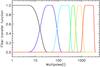 |
Fig. 1 Transfer functions of the 6 wavelet bands used to estimation the CMB with LGMCA. |
 |
Fig. 2 Mask used for the specific processing of the Galactic center. More precisely, the IRIS map is used as an extra observation in the Galactic part of the mask. The sky coverage is about fsky = 82%. |
2.2. Compact sources and Galactic center post-processing
Combining WMAP and Planck is not sufficient to properly clean for compact structures like compact sources, especially on the Galactic center where they can be found in large numbers. The performances of the linear mixture model used so far in LGMCA turns out to be quite limited for extracting these types of contaminants, since it would require far more d.o.f.’s. This limitation can be alleviated by switching to a nonlinear estimator to clean for the compact sources that still contaminate the LGMCA CMB map estimate. Separating the compact sources from the raw CMB map estimate can be recast as a single-observation component separation. This problem is tackled by the MCA (morphological component analysis, Abrial et al. 2007). In this framework, the raw estimate of the CMB map x is assumed to be the linear combination of the compact sources signal xp and the clean CMB map xc: x = xp + xc. From Abrial et al. (2007), emphasizing the morphological differences of the compact sources and the CMB map allows for an accurate separation of both signals. More precisely, the compact sources signal is sparse in the wavelet domain Φ and restricted to compact regions, while the CMB map is homogeneous across the sky and sparsely distributed in the spherical harmonics domain F. The MCA estimate of the compact sources signal xp and the CMB map xc is given by the solution of the following optimization problem: ![Mathematical equation: \begin{equation} \label{eq:mca} \min_{x_{\rm c}, x_{\rm p}} \|x_{\rm c} \vec{F}^{\rm T}\|_1 + \| x_{\rm p} {\bf \Phi}\|_1 \mbox{ s.t. } x = x_{\rm c} + x_{\rm p} ; x_{\rm p}[\Omega] = 0 \end{equation}](/articles/aa/full_html/2014/03/aa22372-13/aa22372-13-eq53.png) (5)where the constraint xp [Ω] = 0 enforces the compact source signal to be zero outside of a prescribed region complementary to Ω. In practice, set Ω and its complement are defined by the compact sources mask and a very restricted region about the Galactic center as displayed in Fig. 3. Interestingly, even if the solution to the problem in Eq. (5) provides solutions that depend nonlinearly on the data x, it provides a linear decomposition via the constraint x = xc + xp. It is also important to notice that pixels of the clean CMB map xc in the sky region Ω remain unaltered by this mechanism.
(5)where the constraint xp [Ω] = 0 enforces the compact source signal to be zero outside of a prescribed region complementary to Ω. In practice, set Ω and its complement are defined by the compact sources mask and a very restricted region about the Galactic center as displayed in Fig. 3. Interestingly, even if the solution to the problem in Eq. (5) provides solutions that depend nonlinearly on the data x, it provides a linear decomposition via the constraint x = xc + xp. It is also important to notice that pixels of the clean CMB map xc in the sky region Ω remain unaltered by this mechanism.
2.3. Map and power spectrum estimation
Following Bobin et al. (2013a), the LGMCA is applied to the five WMAP maps and the nine averages of Planck PR1 half-ring maps so as to estimate the set of mixing matrices. The pseudo inverse of these mixing matrices are then applied to the same WMAP and Planck data to estimate the CMB map. Noise maps are generally derived by applying the pseudo-inverse of the mixing matrices to noise realizations of the data. In the case of WMAP, random noise realizations are computed using the noise covariance matrices that have been provided by the WMAP consortium. For Planck, half differences of half-ring maps provide a good proxy for a single data noise realization.
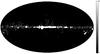 |
Fig. 3 Mask used for the post-processing of the compact sources. The sky coverage is equal to fsky = 97%. |
 |
Fig. 4 Mask used for power spectrum estimation. The sky coverage is equal to fsky = 76%. |
Next in this article, the CMB power spectrum is estimated by computing the cross-correlation between the two half-ring maps. In contrast to the CMB signal, noise decorrelates between half-rings, and the noise bias then vanishes when cross-correlating half-ring maps. Such cross-correlation therefore provides an estimate of the CMB power spectrum, which turns out to be free of any bias from the noise. In the case of WMAP, such virtual half rings maps can be obtained by calculating the difference and sum of the WMAP data and a single data noise realization.
The power spectrum is evaluated from a sky coverage of 76%. Meanwhile, the corresponding mask is composed of a point sources andGalactic maskchosen from the Planck consortium masks.The mask we used for estimating the power spectrum is displayed in Fig. 4. Prior to computing the cross-correlation between the half-ring maps, the maps are deconvolved to infinite resolution up to ℓ = 3200. Changing the resolution of maps is very likely to create artifacts, especially at the vicinity of remaining point sources. To alleviate this problem, the masked map are first in-painted prior to deconvolution. It is important to point out that this stage does not alter the estimation of the power spectrum since it is eventually evaluated from the 76% of the sky, which are kept unchanged through the inpainting step. Correcting for the effect of the mask is made by applying the MASTER mask deconvolution technique (Hivon et al. 2002).
The CMB power spectrum is biased by the contamination of the unresolved point sources, especially at high ℓ > 1500. In Planck Collaboration XV (2014), unresolved point sources are modeled as a contamination with constant power spectrum in each frequency channels. After component separation, the estimated CMB map is computed as a linear combination of the frequency channels. Furthermore, the CMB power spectrum is estimated from regions of the sky (described in Fig. 4) where LGMCA parameters are very likely constant in each wavelet band. As a consequence, the power spectrum of the unresolved point sources will be constant in each of the six wavelet bands. These scalar parameters are denoted by  in sequel.
Following Planck Collaboration XV (2014), an accurate correction of the point source contribution would require estimating the parameters together with the cosmological parameters by maximizing their joint likelihood, but this is beyond the scope of this paper. As first-order correction, these point source parameters are estimated by minimizing the least-square minimization of the error  where Cℓ stands for the estimated power spectrum and
  for the best-fit Planck power spectrum. For instance, the resulting point source parameter in the latest wavelet band (s = 6) takes the value
  for ℓ = 3000 following the convention defined in Planck Collaboration XII (2014). This value is the same order of magnitude as those obtained for other component separation methods in the Planck component separation paper (see the parameter Aps in Fig. 11 of Planck Collaboration XII 2014).
 |
Fig. 5 Left: estimated power spectrum of the WPR1 LGMCA map (red) and official PR1 power spectrum (green). The solid black line is the Planck-only best fit Cℓ provided by the Planck consortium. Right: power spectrum on logarithmic scale. Error bars are set to 1σ. |
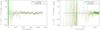 |
Fig. 6 Left: difference between the power spectrum estimated from the WPR1 LGMCA map (red) (resp. official PR1 power spectrum (green)) and the Planck-only best fit Cℓ provided by the Planck consortium. Right: difference between the estimated and theoretical power spectra on logarithmic scale. Error bars are set to 1σ. |
The estimated CMB power spectrum and the official Planck power spectrum are displayed in Fig. 5. The error bars of our estimate of the power spectrum only account for the cosmic variance and noise. Slight differences between the Planck best fit and Planck+WMAP9 power spectra can be seen at very low ℓ. This can be seen with more precision in Fig. 6.
Below, the compatibility of the estimated power spectrum with the official Planck best fit is evaluated. To that end, a standard χ2-based goodness-of-fit procedure and an error tail statistics evaluation are carried out. In the sequel, the error between the estimated and Planck best fit power spectra is defined as  where Vℓ denotes the variance of the estimated power spectrum. In the case of compatibility, the error ℰℓ should be distributed according to a standard normal distribution with mean zero and variance one. This can be tested by computing the error χ2 and the p-value of the resulting value. This test has been carried out on various ranges of multipoles [2,ℓmax] (the monopole and dipole are not taken into account) with ℓmax = 1500, 2000, 2500. The results are displayed in Table 2. The second row of this table features the p value of the χ2 for different ranges of multipoles. The third row (resp. fourth) row shows the number of samples of the normalized error ℰℓ with amplitudes higher than 3σ (resp. higher than 4σ) with respect to the theoretical value (binomial distribution). The probability of the observed number of extreme values, assuming that the error follows a standard Gaussian distribution, is also provided. For ℓ > 1500, the χ2 test do not indicate a good match between the estimated and best-fit Planck power spectra, and the corresponding p values are higher than 0.1.
The evaluation of the tail statistics of the error ℰℓ provides a complementary compatibility test. The third (resp. fourth) row of Table 2 gives the number of samples of ℰℓ with amplitudes higher than 3σ (resp. 4σ). The probability of the observed number of samples follows a binomial distribution with known parameter; this quantity is also provided. For ℓmax ≥ 1500, the observed values are clearly not compatible with the expected theoretical values.
Compatibility check of the estimated power spectrum with the best-fit Planck PR1 from the single ℓ (unbinned) power spectrum.
Compatibility check of the estimated power spectrum with the best-fit Planck PR1 from the binned power spectrum.
This study has been carried out further on the binned power spectrum – displayed in Figs. 5 and 6. The compatibility check results are featured in Table 3. Despite the χ2 values for all ranges of ℓmax, the error ℰℓ exhibits more extreme values than predicted by theory. This indicates that the estimated and best-fit Planck spectra are not compatible.
The discrepancy between the estimated power spectrum and the Planck best fit may have different origins: i) inaccurate error estimation: the uncertainty of the power spectrum should account for the full covariance matrix; ii) inaccurate correction for unresolved point sources and/or CIB; iii) beam transfer function errors at larger ℓ should be taken into account, to only name a few. These different sources of uncertainties will very likely increase the error bars on medium and small scales. Moreover, the error bars of the official power spectrum (Fig. 5) that also includes foreground and beam uncertainties are significantly larger than the error bars estimating in this work cosmic variance and noise only. If the estimated error bars are then substituted with the error bars of the official power spectrum, the χ2 test as well as the tail statistics from the binned power spectrum, no longer indicates any incompatibility – see the values in parenthesis in Table 3. The second row of this table displays the p value of the χ2 for different ranges of multipoles. The third (resp. fourth) row shows the number of samples of the normalized error ℰℓ with amplitudes higher that 3σ (resp. higher than 4σ) with respect to the theoretical value (binomial distribution). The probability of the observed number of extreme values, assuming that the error follows a standard Gaussian distribution, is also provided. The values in parenthesis are obtained by accounting for the error bars of the official power spectrum instead of the error bars derived from noise alone. This suggests that the estimated error bars are probably too optimistic on small scales and should further be updated to account for foreground residuals – namely, point sources and CIB – and instrumental uncertainties.
In the rest of this paper, the CMB map estimated from Planck and WMAP9 will be denoted by WPR1 LGMCA.
3. CMB maps evaluation
This study aims to analyze the joint processing of the WMAP nine-year and Planck PR1 data so as to produce a clean and accurate estimate of the CMB on the entire sky. The larger number of d.o.f.’s allowed by the combination of the WMAP and Planck data should make possible a better cleaning of the Galactic center, as well as prevent the CMB map estimate from SZ residuals. The forthcoming comparisons will therefore precisely focus on evaluating deviations from the expected characteristics of the CMB map through the assessment of various measures of contamination signatures.
3.1. Measuring excess of power with the quality map
Estimating the quality of an estimated CMB map s from real data without any strong assumption about the expected map is challenging. In this section, we assume that the λ-CDM best fit Cℓ provides a power spectrum that gives a good approximation to the expected power of the CMB per frequency. This allows comparing the local deviation around each pixel k in s to this expected power and check whether it is compatible with the expected noise level that the best-fit Cℓ indicates.
This method can be refined by performing this test in the wavelet space rather than in direct space. Given a wavelet function ψ and a given wavelet scale j, one can therefore compute the wavelet coefficients sj = ⟨ ψj, s ⟩. Similarly, one can compute a noise wavelet coefficient nj = ⟨ ψj, n ⟩ from a random noise realization n or the half difference of half ring maps in Planck.
Choosing an isotropic wavelet function, the spherical harmonic coefficients  of
of  are different from zero only for m = 0. The expected CMB power in the band j is then given by
  where Cℓ is the Planck best-fit CMB power spectrum. The local variance of the estimated CMB map on band j and pixel k is performed by calculating the variance of a square patch of size bs × bs pixels centered on pixel k in sj. This procedure yields an estimate of the CMB variance map Sj on each wavelet band j. The same mechanism is utilized to obtain the noise variance maps Nj. In case of a contaminant-free CMB map, the values in the difference map Dj = Sj − Nj should be very close to the expected power Pj of a pure CMB in the wavelet band j up to statistical fluctuations. A strong departure of Dj from Pj would trace the presence of foreground contamination.
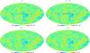 |
Fig. 7 Top: PR1 NILC and SEVEM CMB maps. Bottom: PR1 SMICA and WPR1 LGMCA CMB maps. |
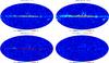 |
Fig. 8 Top: PR1 NILC and SEVEM quality maps. Bottom: PR1 SMICA and WPR1 LGMCA quality maps. |
We define the quality wavelet coefficient for each pixel k as the ratio qj,k = Pj/Dj,k. When qj,k is close to 1, there is no statistically relevant indication of foreground contamination. Conversely, the values of qj,k close to zero suggest the presence of contaminants. The final quality map is obtained by taking the minimum of qj,k across the bands 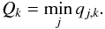 Figure 8 shows the quality maps for four different methods, the three official Planck maps (i.e., NILC, SEVEM, SMICA) and the LGMCA map obtained by jointly processing WMAP nine-year and Planck PR1 data. These maps were generated using the following command line in the open source package iSAP software:
> Q = cmb_qualitymap(CMBmap, NoiseMap, nside=2048,BS=16, NbrScale=4, Cl=Cl).
We plot 1-Q rather than Q, which translates into reading red areas as contaminated regions. The value of Pj was derived from the Planck best-fit cosmological model. It is crucial to note that the fiducial model acts only as a rescaling factor. Therefore using another model would have an extremely low impact on the figures.
Because the SMICA map has a partial sky coverage (a part of the map was inpainted), we set the pixels in Q that turn out to be in-painted to zero. One can observe from Fig. 8 that SEVEM and NILC clearly exhibit much more contamination in the Galactic plane than SMICA and LGMCA. Outside the Galactic plane, none of these maps present significant contamination.
3.2. Galactic center
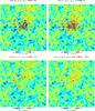 |
Fig. 9 Galactic center region, centered at (l,b) = (80.0,0). Top: PR1 NILC and SEVEM CMB maps, and bottom: PR1 SMICA and WPR1 LGMCA CMB maps. |
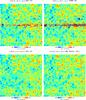 |
Fig. 10 Galactic center region, centered at (l,b) = (37.7,0). Top: PR1 NILC and SEVEM CMB maps; bottom: PR1 SMICA and WPR1 LGMCA CMB maps. |
A glance at the CMB maps in Fig. 7 is mainly significant in the Galactic plane. To visualize these differences better, we show in Figs. 9 and 10 two regions in the Galactic center. In both cases, the maps stemming only from the processing of Planck all exhibit significant foreground residuals. Conversely, the LGMCA map does not present any visible remaining foreground emission. The very clean aspect of the Galactic center can be explained by the flexibility that the joint processing of WMAP and Planck allows for separating foreground components, as well as for the efficiency in the post-processing of the compact sources.
3.3. SZ contamination
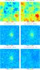 |
Fig. 11 Coma cluster area. Top: PR1 LGMCA CMB map and HFI-217 GHz map. Middle and bottom: difference map between HFI-217 GHz and CMB maps, PR1 NILC, SEVEM, SMICA, and WPR1 LGMCA respectively. |
The quality maps displayed in Fig. 8 show that the CMB maps do not exhibit significant foreground contamination outside of the Galactic center. Differences between the maps can only be measured at the Galactic center. At higher Galactic latitude, potential contamination seems to be well below the CMB fluctuations, which makes them challenging to detect.
Fortunately, one potential foreground contamination that can be evaluated is the thermal Sunyaev Zel’Dovich (tSZ) effect. An interesting property of the tSZ effect is that it almost vanishes at 217 GHz, and its contribution can considered negligible in this band. Therefore the difference between the HFI-217 GHz channel map and a clean CMB map should cancel out the CMB without revealing tSZ contamination. Conversely, the same difference with a tSZ contaminated map should exhibit the remaining tSZ contamination.
To illustrate this, Fig. 11 shows the difference maps of the four CMB maps with the HFI-217GHz channel map. It appears clearly that three of the maps have tSZ contamination: the Coma cluster can be well detected. Conversely, the LGMCA map does not present any tSZ contamination. This is expected because the LGMCA method takes the SZ emission explicitly into account during the component separation, which therefore prevents the CMB map estimate from being subject to tSZ contamination. This qualitative study can be complemented further by evaluating the level of tSZ and kSZ residuals in the CMB estimated from Planck sky model simulations that assume that the electromagnetic spectrum of tSZ is perfectly known. These simulations are described in Sect. A. The contribution of the kSZ and tSZ can be estimated by applying the LGMCA parameters to the individual contribution of the kSZ and tSZ emission in the simulated frequency channels. Figure 12 displays the power spectra of the kSZ and tSZ residual contamination in the estimated CMB as well as the CMB power spectrum. Interestingly, this figure shows that the tSZ residual has a contribution that can be neglected with respect to kSZ. According to these simulations, this makes the LGMCA CMB map a good candidate for kinetic SZ studies.
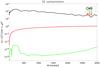 |
Fig. 12 tSZ and kSZ residuals in spherical harmonics in the CMB map estimated by LGMCA from simulated Planck+WMAP data. |
3.4. Assessment of the foreground contamination level
In the absence of accessible public sets of realistic simulations of the Planck sky processed by all component separation methods, assessing how foregrounds propagate to the final CMB estimates is challenging, so such an analysis should be performed with the greatest care. The main difficulties in quantitatively comparing maps rely on 1) a slightly different resolution for each map; 2) the masking performed on NILC and SMICA maps close to the Galactic center that prevents full-sky comparisons; and 3) the respective levels of CMB and noise make it difficult to estimate residual contamination (however indicating a successful source separation over a large portion of the sky).
To address the masking issue, all maps were first inpainted in the combined SMICA and NILC small masks (retaining 97% of the sky) using the sparse inpainting technique described in Abrial et al. (2007). These maps can then be analyzed on various wavelet bands with little impact from the masked region. The maps were degraded afterward to a common resolution of five arcminutes with an additional low-pass filter to limit the ringing of strong compact emissions.
3.4.1. Cross-correlation with external templates
Computing quantitative measures of foreground contamination from real data is not trivial. One way of measuring differences in foreground levels between CMB maps can be carried out through their cross-correlation with external templates that trace specific foreground emissions. Such cross-correlations have been performed with the Haslam 408 MHz map, an H-alpha template provided by the WMAP consortium (see Bennett 2013), an HI column density map, a velocity-integrated CO brightness temperature map (all accessible via the NASA website1), and the IRIS 100μm map (Miville-Deschênes & Lagache 2005). A set of 80 realizations of CMB maps (assuming the fiducial cosmological model obtained from the Planck PR1 results) and noise maps were also processed through the LGMCA pipeline. Statistics obtained from the CMB maps were normalized by the standard deviation of the statistics computed from the noise realizations. Since these noise realizations are only valid for the WPR1 LGMCA map (in the absence of similar propagated noise realizations for other component separation methods available), this normalized correlation should be understood as a rescaling between the different wavelet bands, and the amplitude only as a very rough approximation of the correlation signal-to-noise ratio. Figure 13 shows the normalized correlation for different CMB maps, the three released Planck PR1 maps (i.e., NILC, SMICA, SEVEM), the WPR1 LGMCA map, and the PR1 LGMCA map. The latest is shown in order to see whether adding WMAP-9 yr channels improves the cross-correlation with the different templates. We can see that none of these plots exhibit statistically significant cross-correlations (i.e., normalized correlation greater than five), with the exception of the finest band in the one calculated with the IRIS map. This cross-correlation could be attributed to dust or CIB. Investigating this effect more, we have seen that this strong correlation on fine scales in the SEVEM map disappears when we use the 70% fsky mask provided with the SEVEM map, which means it could be due to either unmasked infrared-point sources in the small combined SMICA and NILC mask, or residual dust in the Galactic center that remains in the SEVEM map. Concerning the WPR1 LGMCA map, the same experience did not remove this effect, so the contamination is most likely due to CIB.
3.4.2. Higher order statistics
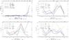 |
Fig. 13 Normalized cross-correlation per wavelet band of the CMB maps with the IRIS map (top left), the Haslam map (top right), the H1 map (bottom left) and the free-free template (bottom right). |
 |
Fig. 14 Normalized high order statistics computed on various wavelet bands for the high resolution masks inside the in-painting mask (about 97% of the sky): Skewness (top left), Kurtosis (top right), cumulant of orders 5 and 6 (bottom left and right). |
Deviations from Gaussianity is another way to quantify the level of remaining foregrounds without requiring ancillary templates. For that purpose, higher order statistics provide a model-independent measure of non-Gaussianity (NG), which can be further enhanced when evaluated in the wavelet domain. Figure 14 shows the skewness, the kurtosis, and the cumulants of orders 5 and 6. These values are computed using the same sky coverage as in the previous section, and are normalized in a similar way. We can see that strong departures from Gaussianity is observed on the first two bands. To better characterize these NG, we have also performed the same analysis but per latitude band. Figure 15 (top) shows the normalized kurtosis on bands 1 and 2, and Fig. 15 bottom shows the normalized cumulant of order 6 on bands 1 and 2.
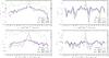 |
Fig. 15 Normalized high order statistics per latitude band computed from the two finest wavelet scales for the high resolution masks inside the inpainting mask (about 97% of the sky): top: normalized Kurtosis on bands 1 and 2, and bottom: normalized cumulant of order 6 on bands 1 and 2. |
From this evaluation, we can conclude that
-
All maps are compatible with the Gaussianity assumption up tothe second wavelet scale.
-
LGMCA maps (PR1 and WPR1) present the best behavior on the finest bands. This is also an indication that the contamination shown in the previous detection is instead due to CIB, since dust contamination would have certainly impacted the high order statistics.
-
Deviation from Gaussianity is significant for all maps, but only on the finest bands. These NG are clearly due to foreground residuals in the Galactic plane, except for SEVEM where point sources contaminate the map more and need to be masked. This confirms that a much more conservative mask is required for cosmological non-Gaussianity studies, especially when the finest scales are used, such as for CMB weak lensing or fnl detection.
-
Point source processing methods that were used for all maps, except SEVEM, seem to work properly outside the Galactic plane, since no NG are detected.
3.4.3. WPR1 versus PR1
The differences between the WPR1 LGMCA map and the currently available maps can have many origins that go beyond the joint processing with the WMAP data: i) sparsity is used as a separation criterion; ii) post-processing of the point sources and the Galactic center. From our tests, the differences between the WPR1 LGMCA and PR1 LGMCA maps, obtained by performing LGMCA on the Planck data alone, are relatively slight. The main one concerns the correlation with the H1 template, where on band 6, the PR1 map presents a significant cross-corrrelation with the H1 template (about 4σ detection), while this quantity remains insignificant for the WPR1 LGMCA map.
List of products made available in this paper in the spirit of reproducible research, available here: http://www.cosmostat.org/planck_wpr1.html.
Another interesting aspect relative to the joint reconstruction is that residual systematics in Planck and WMAP are likely to be unrelated. From this perspective, we can expect that combining the Planck and WMAP data would lead to a CMB with fewer systematics (Planck Collaboration 2014; Frejsel et al. 2013; Naselsky et al. 2012; Gruppuso et al. 2013). This should be the case especially for the largest scales of the CMB map where correcting for the systematic effects is particularly challenging. This suggests that a study of the large scale multipoles of the CMB map should be thoroughly performed, which we leave for future work.
4. Reproducible research
In the spirit of participating in reproducible research, we have made all codes and resulting products that constitute the main results of this paper public. In Table 4 we list all the products that are made freely available as a result of this paper and which are available here: http://www.cosmostat.org/planck_wpr1.html.
5. Conclusion
We combined the WMAP nine-year and Planck PR1 data to produce a clean full-sky CMB map (without inpainted or interpolated pixels). The joint processing of the WMAP and Planck was carried out by a recently introduced sparsity-based component separation method called LGMCA. It also benefits from an effective post-processing of point sources based on the MCA. We showed that this processing yields a full-sky CMB map with no significant foreground residuals in the Galactic center. Moreover, the larger number of d.o.f.’s due to the joint processing of WMAP and Planck allows estimating a map without detectable tSZ contamination, in contrast to existing available CMB maps. Our conclusions relative to the WPR1 LGMCA CMB map are that it
-
is the only one that is full-sky, without requiring any inpaintingtechniques;
-
is virtually free of tSZ contamination, so it should be the best candidate for the kSZ studies;
-
is very clean, even in theGalactic plane;
-
presents, however, a slightly higher CIB contamination detectable for l > 2000;
-
assuming the power spectrum of the LGMCA CMB map is similar has error bars which are similar to those estimated by the Consortium, taking all instrumental effects and residual foregrounds into account (beam uncertainties, point sources, CIB, etc), the GMCA estimated power spectra does not show any discrepancy with the Planck best-fit power spectrum.
-
presents a slightly lower level of H1 contamination than the PR1 map, while exhibiting no statistically significant differences otherwise.
This suggests that further study should emphasize the analysis of the large scale structure of the CMB from the PR1 LGMCA and WPR1 LGMCA maps.
Online material
Appendix A: Simulations
Simulated data
The LGMCA algorithm is applied to the WMAP and Planck data, which is simulated by the Planck Sky Model5 (PSM; Delabrouille et al. 2013). The PSM models the instrumental noise, the beams, and the astrophysical foregrounds in the frequency range that is probed by WMAP and Planck. The simulations were obtained as follows:
-
Frequency channels: the simulated data contains the 14 WMAP andPlanck frequency channels ranging from 23to 857 GHz. The frequency-dependent beams are assumed to be isotropic Gaussian PSFs.
-
Instrumental noise: instrumental noise has been generated according to a Gaussian distribution, with a covariance matrix provided by the WMAP (9-year) and the Planck consortia.
-
Cosmic microwave background: the CMB map is drawn from a Gaussian random field with WMAP 9-year best-fit theoretical power spectrum (from the 6 cosmological parameters model). No non-Gaussianities, such as lensing or ISW effects, have been added to the CMB map.
-
Synchrotron: this emission arises from the acceleration of the cosmic-ray electrons in the magnetic field of our Galaxy. It follows a power law with a spectral index that varies across pixels from −3.4 and −2.3 (Bennett et al. 2003). In the Planck data, this component mainly appears at lower frequency observations (typ. ν < 70 GHz).
-
Free-Free: the free-free emission is due to the electron-ion scattering and follows a power law distribution with an almost constant spectral index across the sky (~-2.15) (Dickinson et al. 2003).
-
Dust emission: this component arises from the thermal radiation of the dust grains in the Milky Way. It follows a gray-body spectrum that depends on two parameters: the dust temperature and the spectral index (Finkbeiner et al. 1999). Recent studies that involve the joint analysis of IRIS and Planck 545 and 857 Ghz observations show significant variations in both the dust temperature and the spectral index across the sky on both large and small scales (Planck Collaboration 2011a).
-
AME: the AME (anomalous microwave emission) – or spinning dust – may develop from the emission of spinning dust grains. This component has a spatial correlation with the thermal dust emission but has an emissivity that roughly follows a power law in the frequency range of Planck and WMAP (Planck Collaboration 2011b).
-
CIB: cosmological infrared background comes from the emission of unresolved galaxies at high redshifts.
-
CO: CO emission has been simulated using the DAME H1 line survey (Dame et al. 2001).
-
SZ: the Sunyaev-Zel’Dovich effect results from the interactions of the high energy electrons and the CMB photons through inverse Compton scattering (Sunyaev & Zeldovich 1970). The SZ electromagnetic spectrum is well known to be constant across the sky.
-
Point sources: these components belong to two categories of radio and infra-red point sources, which can have Galactic or extra-Galactic origins. Most of the brightest compact sources are found in the ERCSC catalog provided by the Planck mission (Planck Collaboration 2011c). These point sources have individual electromagnetic spectra.
The same IRIS 100 μm map and parameters, as listed in Table 1, were used for LGMCA.
Recovered maps
The recovered CMB map is displayed in Fig. A.1. The error map, defined as the difference between the estimated and the input CMB maps, is shown in Fig. A.2. For a better visualization of the foreground residuals, the error map has been downgraded to a resolution of 1.5 degrees. The error map contains some traces of instrumental noise as well as some foreground residuals. Apart from some of the point sources at high latitudes, most foreground residuals seem to be concentrated in the vicinity of the Galactic center, which is expected.
To evaluate the quality of our estimated CMB map, the correlation coefficient of the estimated CMB map with the input foregrounds has been calculated and is displayed in Fig. A.3. Apart from the CIB, none of the foreground components have a correlation coefficient that exceeds 0.05. Interestingly, as conjectured from the analysis of the Planck PR1 data in Sect. 3.4.2, the CIB contamination increases on small scales with the correlation coefficient reaching to about 0.3. In this evaluation, no mask has been used to obtain a full-sky CMB map estimate.
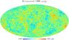 |
Fig. A.1 CMB estimated from simulated WMAP and Planck data. |
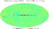 |
Fig. A.2 Residual map defined as the difference between the estimated CMB and the true simulated CMB map at resolution 1.5 degree. |
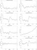 |
Fig. A.3 Correlation coefficient in the harmonic space of the input foregrounds with the estimated CMB map. Error bars are set to 1σ and computed from 50 Monte-Carlo simulations of CMB + noise. |
Assessing the uncertainty of the estimated CMB map
Uncertainty estimation from simulations:
even if the foregrounds have been properly removed from the estimated map, we have to weigh the pixels in the map by the variance of the estimator. This would require performing Monte-Carlo simulations for all the components that compose the data, i.e. the CMB, the instrumental noise, and the foregrounds, which are clearly unavailable. A more practical approach is to derive an uncertainty map that relies on measuring the variance from the error map – displayed in Fig. A.2.
We define  as the estimator variance in the pixel domain and propose estimating by the local variance of the error map. As a result, the uncertainty map, featured in Fig. A.4, has been computed by measuring the variance of the error map on overlapping patches of size 16 × 16 pixels. This particularly assumes that the uncertainty is stationary within each patch. As expected, with the exception of the point sources, the uncertainty map is mainly dominated by instrumental noise at high latitudes and by foreground residuals in the vicinity of the Galactic center. We then define the normalized error by
 ![Mathematical equation: \appendix \setcounter{section}{1} \begin{eqnarray*} \mbox{for each pixel } k, \quad \epsilon[k] = \frac{\hat{x}[k] - x^\star[k] }{\sqrt{\mathcal{V}[k]}}, \end{eqnarray*}](/articles/aa/full_html/2014/03/aa22372-13/aa22372-13-eq166.png) where x̂ stands for the estimated CMB map, and x⋆ is the input one. A proper estimation of should be such that the normalized error ϵ asymptotically follows a Gaussian distribution with mean zero and variance one (standard normal distribution). The histogram of the normalized error is shown in Fig. A.5. The resulting normalized error is indeed close to a standard normal distribution.
where x̂ stands for the estimated CMB map, and x⋆ is the input one. A proper estimation of should be such that the normalized error ϵ asymptotically follows a Gaussian distribution with mean zero and variance one (standard normal distribution). The histogram of the normalized error is shown in Fig. A.5. The resulting normalized error is indeed close to a standard normal distribution.
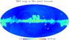 |
Fig. A.4 Uncertainty map of the estimated CMB map in the pixel domain. |
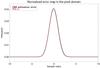 |
Fig. A.5 Histogram of the normalized error map in the pixel domain (solid black curve) and standard normal distribution (dotted red curve). |
The foreground and the instrumental noise residuals are expected to be spatially correlated and, therefore, cannot be characterized well in the pixel domain. It can be complemented by evaluating the uncertainty in the spherical harmonics domain. Assuming that the expected uncertainty is isotropic, the CMB map uncertainty can be approximated by the power spectrum of the error map, in other words by the variance of its spherical harmonics coefficients, or aℓm. The resulting power spectrum  is shown in Fig. A.6. As in the pixel domain, one can compute the normalized error in spherical harmonics:
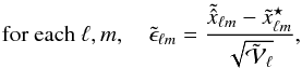 where
where
 and
and  stand for the spherical harmonics coefficients of the estimated and the input CMB maps. The histogram of the normalized error in the spherical harmonics domain is shown in Fig. A.7. As expected, the error distribution is close to a standard normal distribution.
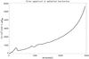 |
Fig. A.6 Uncertainty spectrum of the estimated CMB map in the harmonic domain. |
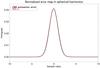 |
Fig. A.7 Histogram of the normalized error map in the harmonic domain (solid black curve) and standard normal distribution (dotted red curve). |
Case of real data:
the accurate estimation of the CMB map uncertainty is very challenging in the case of real data because it is quite complex to estimate the errors at the level of CMB fluctuations or below. The quality map derived in Sect. 3 can only capture errors that are above the average noise level in the wavelet domain but is not sensitive to errors that lie below the CMB fluctuations.
There are two sources of error that can contaminate the CMB: i) remaining instrumental noise; ii) foreground residuals. For real data, the contribution of the remaining instrumental noise to the estimate of the total error of the CMB map can be derived by computing the local variance of the half-ring difference. However, as explained previously, estimating the level of foreground residuals in the final map can only be obtained by performing simulations. In reality, simulations are only reliable on large scales where the sky has been accurately observed and studied. Therefore, we propose two approaches to estimating the uncertainty of the estimated CMB map on large scales:
-
Conservative estimate: apart from the point source resid-ual, the level of foreground residuals increases towards theGalactic center. A conservative approach is to estimate thelevel of foreground residuals from simulations by com-puting the variance of the error map in bands of latitudesof 0.25 degrees. The total error esti-mate, shown in Fig. A.8, is then obtained by addingthe resulting foreground residual variance and the noise variancederived from WMAP noise simulations and the Planck half ringdifference. This error map provides a rough estimate of the erroracross latitude but is not an accurate estimate along the longitude,specifically around the Galactic center where the error variationsalong the longitude is not small. This map will be made availableas a product (see Sect. 4).
-
Large-scale estimate: the latest version of the Planck sky model (PSM) includes physical models for the foreground components, which have been derived from the various Galactic studies. Therefore, the PSM is quite reliable at resolutions where the sky is accurately studied (i.e. resolutions greater than about 1 degree). We can therefore estimate the level of the foreground residual by computing the local variance of the error map smoothed at one degree resolution. The final error estimate, shown in Fig. A.9, is then obtained by adding the resulting foreground variance and the noise variance derived from WMAP noise simulations and the Planck half ring difference.
These maps provide a rough idea of the level of uncertainty of the CMB map, which also help to define reliable regions for further studies (non-Gaussianities, power spectrum estimation, etc.).
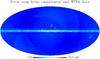 |
Fig. A.8 Uncertainty map estimated by combining a level of foreground residuals estimated in bands of latitudes and the level of noise from WMAP and Planck data. |
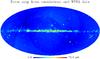 |
Fig. A.9 Uncertainty map estimated by combining a level of foreground residuals at one degree resolution and the level of noise from WMAP and Planck data. |
For more details please visit the PSM website: http://www.apc.univ-paris7.fr/~delabrou/PSM/psm.html.
Acknowledgments
We would like to thank the anonymous reviewer for his comments that greatly helped in improving the paper. This work is supported by the European Research Council grant SparseAstro (ERC-228261), by the Centre National des Etudes Spatiales (CNES), and by the Swiss National Science Foundation (SNSF). We used Healpix software (Gorski et al. 2005), iSAP2 software, WMAP data3, and Planck data4.
References
- Abrial, P., Moudden, Y., Starck, J., et al. 2007, J. Fourier Anal. Appl., 13, 729 [Google Scholar]
- Basak, S., & Delabrouille, J. 2012, MNRAS, 419, 1163 [NASA ADS] [CrossRef] [Google Scholar]
- Bennett, C. L., Hill, R. S., Hinshaw, G., et al. 2003, ApJS, 148, 97 [NASA ADS] [CrossRef] [Google Scholar]
- Bennett, C. L., Larson, D., Weiland, J. L., et al. 2013, ApJS, 208, 20 [Google Scholar]
- Bobin, J., Starck, J.-L., Sureau, F., & Basak, S. 2013a, A&A, 550, A73 [NASA ADS] [CrossRef] [EDP Sciences] [Google Scholar]
- Bobin, J., Sureau, F., Paykari, P., et al. 2013b, A&A, 553, L4 [NASA ADS] [CrossRef] [EDP Sciences] [Google Scholar]
- Bouchet, R., & Gispert, R. 1999, New Astron., 4 [Google Scholar]
- Dame, T. M., Hartmann, D., & Thaddeus, P. 2001, ApJ, 547, 792 [NASA ADS] [CrossRef] [Google Scholar]
- Delabrouille, J., Cardoso, J.-F., & Patanchon, G. 2003, MNRAS, 346, 1089 [NASA ADS] [CrossRef] [Google Scholar]
- Delabrouille, J., Cardoso, J.-F., Jeune, M. L., et al. 2009, A&A, 493, 835 [NASA ADS] [CrossRef] [EDP Sciences] [Google Scholar]
- Delabrouille, J., Betoule, M., Melin, J.-B., et al. 2013, A&A, 553, A96 [NASA ADS] [CrossRef] [EDP Sciences] [Google Scholar]
- Dickinson, C., Davies, R., & Davis, R. 2003, MNRAS, 341 [Google Scholar]
- Eriksen, H. K., Jewell, J. B., Dickinson, C., et al. 2008, ApJ, 676, 10 [NASA ADS] [CrossRef] [Google Scholar]
- Fernández-Cobos, R., Vielva, P., Barreiro, R. B., & Martínez-González, E. 2012, MNRAS, 420, 2162 [NASA ADS] [CrossRef] [Google Scholar]
- Finkbeiner, D., Davis, M., & Schlegel, D. 1999, ApJ, 524 [Google Scholar]
- Frejsel, A., Hansen, M., & Liu, H. 2013, J. Cosmol. Astropart. Phys., 6, 5 [NASA ADS] [CrossRef] [Google Scholar]
- Gold, B., Odegard, N., Weiland, J. L., et al. 2011, APJS, 192, 15 [NASA ADS] [CrossRef] [Google Scholar]
- Gorski, K., Hivon, E., Banday, A. J., et al. 2005, ApJ, 622 [Google Scholar]
- Gruppuso, A., Natoli, P., Paci, F., et al. 2013, J. Cosmol. Astropart. Phys., 7, 47 [Google Scholar]
- Hivon, E., Górski, K. M., Netterfield, C. B., et al. 2002, ApJ, 567, 2 [NASA ADS] [CrossRef] [Google Scholar]
- Leach, S. M., Cardoso, J.-F., Baccigalupi, C., et al. 2008, A&A, 491 [Google Scholar]
- Miville-Deschênes, M.-A., & Lagache, G. 2005, ApJS, 157, 302 [NASA ADS] [CrossRef] [Google Scholar]
- Naselsky, P., Zhao, W., Kim, J., & Chen, S. 2012, ApJ, 749, 31 [NASA ADS] [CrossRef] [Google Scholar]
- Planck Collaboration 2011a, A&A, 536, A19 [NASA ADS] [CrossRef] [EDP Sciences] [Google Scholar]
- Planck Collaboration 2011b, A&A, 536, A20 [NASA ADS] [CrossRef] [EDP Sciences] [Google Scholar]
- Planck Collaboration 2011c, A&A, 536, A7 [NASA ADS] [CrossRef] [EDP Sciences] [Google Scholar]
- Planck Collaboration XII. 2014, A&A, in press, DOI: 10.1051/0004-6361/201321580 [Google Scholar]
- Planck Collaboration XV. 2014, A&A, submitted [arXiv:1303.5075] [Google Scholar]
- Planck Collaboration XXIII. 2014, A&A, in press, DOI: 10.1051/0004-6361/201321534 [Google Scholar]
- Starck, J.-L., Donoho, D. L., Fadili, M. J., & Rassat, A. 2013, A&A, 552, A133 [NASA ADS] [CrossRef] [EDP Sciences] [Google Scholar]
- Sunyaev, R. A., & Zeldovich, Y. B. 1970, Astrophys. Space Sci., 7, 3 [Google Scholar]
All Tables
Compatibility check of the estimated power spectrum with the best-fit Planck PR1 from the single ℓ (unbinned) power spectrum.
Compatibility check of the estimated power spectrum with the best-fit Planck PR1 from the binned power spectrum.
List of products made available in this paper in the spirit of reproducible research, available here: http://www.cosmostat.org/planck_wpr1.html.
All Figures
|
Fig. 1 Transfer functions of the 6 wavelet bands used to estimation the CMB with LGMCA. |
| In the text | |
|
Fig. 2 Mask used for the specific processing of the Galactic center. More precisely, the IRIS map is used as an extra observation in the Galactic part of the mask. The sky coverage is about fsky = 82%. |
| In the text | |
|
Fig. 3 Mask used for the post-processing of the compact sources. The sky coverage is equal to fsky = 97%. |
| In the text | |
|
Fig. 4 Mask used for power spectrum estimation. The sky coverage is equal to fsky = 76%. |
| In the text | |
|
Fig. 5 Left: estimated power spectrum of the WPR1 LGMCA map (red) and official PR1 power spectrum (green). The solid black line is the Planck-only best fit Cℓ provided by the Planck consortium. Right: power spectrum on logarithmic scale. Error bars are set to 1σ. |
| In the text | |
|
Fig. 6 Left: difference between the power spectrum estimated from the WPR1 LGMCA map (red) (resp. official PR1 power spectrum (green)) and the Planck-only best fit Cℓ provided by the Planck consortium. Right: difference between the estimated and theoretical power spectra on logarithmic scale. Error bars are set to 1σ. |
| In the text | |
|
Fig. 7 Top: PR1 NILC and SEVEM CMB maps. Bottom: PR1 SMICA and WPR1 LGMCA CMB maps. |
| In the text | |
|
Fig. 8 Top: PR1 NILC and SEVEM quality maps. Bottom: PR1 SMICA and WPR1 LGMCA quality maps. |
| In the text | |
|
Fig. 9 Galactic center region, centered at (l,b) = (80.0,0). Top: PR1 NILC and SEVEM CMB maps, and bottom: PR1 SMICA and WPR1 LGMCA CMB maps. |
| In the text | |
|
Fig. 10 Galactic center region, centered at (l,b) = (37.7,0). Top: PR1 NILC and SEVEM CMB maps; bottom: PR1 SMICA and WPR1 LGMCA CMB maps. |
| In the text | |
|
Fig. 11 Coma cluster area. Top: PR1 LGMCA CMB map and HFI-217 GHz map. Middle and bottom: difference map between HFI-217 GHz and CMB maps, PR1 NILC, SEVEM, SMICA, and WPR1 LGMCA respectively. |
| In the text | |
|
Fig. 12 tSZ and kSZ residuals in spherical harmonics in the CMB map estimated by LGMCA from simulated Planck+WMAP data. |
| In the text | |
|
Fig. 13 Normalized cross-correlation per wavelet band of the CMB maps with the IRIS map (top left), the Haslam map (top right), the H1 map (bottom left) and the free-free template (bottom right). |
| In the text | |
|
Fig. 14 Normalized high order statistics computed on various wavelet bands for the high resolution masks inside the in-painting mask (about 97% of the sky): Skewness (top left), Kurtosis (top right), cumulant of orders 5 and 6 (bottom left and right). |
| In the text | |
|
Fig. 15 Normalized high order statistics per latitude band computed from the two finest wavelet scales for the high resolution masks inside the inpainting mask (about 97% of the sky): top: normalized Kurtosis on bands 1 and 2, and bottom: normalized cumulant of order 6 on bands 1 and 2. |
| In the text | |
|
Fig. A.1 CMB estimated from simulated WMAP and Planck data. |
| In the text | |
|
Fig. A.2 Residual map defined as the difference between the estimated CMB and the true simulated CMB map at resolution 1.5 degree. |
| In the text | |
|
Fig. A.3 Correlation coefficient in the harmonic space of the input foregrounds with the estimated CMB map. Error bars are set to 1σ and computed from 50 Monte-Carlo simulations of CMB + noise. |
| In the text | |
|
Fig. A.4 Uncertainty map of the estimated CMB map in the pixel domain. |
| In the text | |
|
Fig. A.5 Histogram of the normalized error map in the pixel domain (solid black curve) and standard normal distribution (dotted red curve). |
| In the text | |
|
Fig. A.6 Uncertainty spectrum of the estimated CMB map in the harmonic domain. |
| In the text | |
|
Fig. A.7 Histogram of the normalized error map in the harmonic domain (solid black curve) and standard normal distribution (dotted red curve). |
| In the text | |
|
Fig. A.8 Uncertainty map estimated by combining a level of foreground residuals estimated in bands of latitudes and the level of noise from WMAP and Planck data. |
| In the text | |
|
Fig. A.9 Uncertainty map estimated by combining a level of foreground residuals at one degree resolution and the level of noise from WMAP and Planck data. |
| In the text | |
Current usage metrics show cumulative count of Article Views (full-text article views including HTML views, PDF and ePub downloads, according to the available data) and Abstracts Views on Vision4Press platform.
Data correspond to usage on the plateform after 2015. The current usage metrics is available 48-96 hours after online publication and is updated daily on week days.
Initial download of the metrics may take a while.