| Issue |
A&A
Volume 563, March 2014
|
|
|---|---|---|
| Article Number | A142 | |
| Number of page(s) | 11 | |
| Section | Catalogs and data | |
| DOI | https://doi.org/10.1051/0004-6361/201321654 | |
| Published online | 25 March 2014 | |
Deep R-band counts of z ≈ 3 Lyman-break galaxy candidates with the LBT⋆,⋆⋆
1 INAF – Osservatorio Astronomico di Roma, via Frascati 33, 00040 Monteporzio (RM), Italy
e-mail: konstantina.boutsia@oa-roma.inaf.it
2 INAF – Osservatorio Astronomico di Bologna, via Ranzani 1, 40127 Bologna, Italy
Received: 5 April 2013
Accepted: 12 November 2013
Aims. We present a deep multiwavelength imaging survey (UGR) in 3 different fields, Q0933, Q1623, and COSMOS, for a total area of ~1500 arcmin2. The data were obtained with the Large Binocular Camera on the Large Binocular Telescope.
Methods. To select our Lyman-break galaxy (LBG) candidates, we adopted the well established and widely used color-selection criterion (U − G vs. G − R). One of the main advantages of our survey is that it has a wider dynamic color range for U-dropout selection than in previous studies. This allows us to fully exploit the depth of our R-band images, obtaining a robust sample with few interlopers. In addition, for 2 of our fields we have spectroscopic redshift information that is needed to better estimate the completeness of our sample and interloper fraction.
Results. Our limiting magnitudes reach 27.0(AB) in the R band (5σ) and 28.6(AB) in the U band (1σ). This dataset was used to derive LBG candidates at z ≈ 3. We obtained a catalog with a total of 12 264 sources down to the 50% completeness magnitude limit in the R band for each field. We find a surface density of ~3 LBG candidates arcmin-2 down to R = 25.5, where completeness is ≥95% for all 3 fields. This number is higher than the original studies, but consistent with more recent samples.
Key words: surveys / catalogs / galaxies: high-redshift / galaxies: photometry / ultraviolet: galaxies
Observations were carried out using the Large Binocular Telescope at Mt. Graham, AZ. The LBT is an international collaboration among institutions in the United States, Italy, and Germany. LBT Corporation partners are The University of Arizona on behalf of the Arizona university system; Istituto Nazionale di Astrofisica, Italy; LBT Beteiligungsgesellschaft, Germany, representing the Max-Planck Society, the Astrophysical Institute Potsdam, and Heidelberg University; The Ohio State University; and The Research Corporation, on behalf of The University of Notre Dame, University of Minnesota, and University of Virginia.
Full Tables A.1–A.3 are only available at the CDS via anonymous ftp to cdsarc.u-strasbg.fr (130.79.128.5) or via http://cdsarc.u-strasbg.fr/viz-bin/qcat?J/A+A/563/A142
© ESO, 2014
1. Introduction
Lyman-break galaxies (LBGs) are star-forming galaxies that emit very little flux in the observed UV when they are at redshifts higher than z = 2.5. This is because the stellar radiation with energy beyond the Lyman limit (912 Å) is absorbed by the surrounding neutral hydrogen and by the intervening neutral clouds between the galaxy and the observer. Thus the spectral energy distributions (SEDs) of these galaxies are characterized by a sharp drop at wavelengths shorter than the 912 Å rest frame (Madau 1995) and by a steep increase between the 912 Å and the 1216 Å rest frame. Such features have been used extensively during past decades to create substantial samples of LBGs at high redshifts. More specifically, the filters UGR have been used for selecting U dropouts that are candidate LBGs at z ≈ 3 (e.g., Steidel et al. 1996, 2003; Giavalisco 2002; Capak et al. 2004; Sawicki & Thompson 2005; Nonino et al. 2009). Steidel et al. (2003) applied this method to 17 high Galactic-latitude fields and presented a sample of 2347 photometrically selected LBG candidates down to a magnitude limit of 25.5 in the R band, corresponding to ~1500 Å rest frame at z ≈ 3, in an area of ~3200 arcmin2. After a spectroscopic follow-up (Steidel et al. 2004), the success rate for LBGs at redshift z ~ 3 was on the order of 78%. Thus the adopted color selection provides samples with low contamination that can be used for spectroscopic follow up to do statistical analyses of the LBG population and to study the physical properties of LBGs, such as stellar masses and the UV slope. A statistically significant LBG sample, associated with deep U-band imaging, can also be used to derive stringent upper limits for the escape fraction of UV ionizing radiation from LBGs. In addition, such a dataset is suitable for studying clustering by applying a two-point correlation function analysis, as well as for deriving the fraction of active galactic nuclei embedded in such galaxies by combining it with X-ray observations.
After the first effort by Steidel et al. (2003), similar surveys have been conducted that reach different magnitude limits. Sawicki & Thompson (2005) covered a relatively small area (169 arcmin2), but reached a deeper magnitude limit of R = 27.0 (50% point sources detected). More recently, Rafelski et al. (2009) presented a sample of LBGs at z ~ 3, using both photometric redshifts and color selection. Their color-selection criterion uses a filter set that is slightly different (u − V vs. V − z) from the one established by Steidel et al. (2003) (U − G vs. G − R), and their sample is complete up to V ≈ 27.0, which corresponds to R ≈ 26.5 for this type of sources. Nonino et al. (2009) present deep imaging in the GOODS area (630 arcmin2), with 50% completeness in LBG selection at R ≈ 26.0. Ly et al. (2011) used Subaru images, covering an area of 870 arcmin2, with 5σ limiting magnitudes of R = 27.3, but limited the search for LBG candidates at R = 25.5. An extended survey has been presented by van der Burg et al. (2010), who used data from the Deep CFHT survey, which covers 4 sq. deg and reaches R = 27.9 at 5σ, although their U-dropout number counts only seem to be complete up to R = 26.0. The most recent and extended survey is the one conducted by Bian et al. (2013), which covers 9 sq. deg in the NOAO Bo tes Field, although it is rather shallow, selecting LBG candidates down to R = 25.0.
Because of the variety of instruments and filters used to select these LBG candidates at z ~ 3, the selection biases in the various samples are difficult to quantify and at times they lead to diverging results. For example, Le Fèvre et al. (2005) find that the number density of galaxies between z = 1.4 and z = 5 is 1.6 to 6.2 times higher than earlier estimates based mainly on the work of Steidel et al. (2004). Such discrepancies in the number density also lead to discrepancies in the derived LFs (e.g., Iwata et al. 2007; Sawicki & Thompson 2006; Reddy et al. 2008).
We used the Large Binocular Camera (LBC, Giallongo et al. 2008) at the Large Binocular Telescope (LBT) to obtain a multiwavelength dataset (UGRIZ) on three different fields to derive a new sample of LBG candidates at z ~ 3 through photometric selection. One of the main advantages of our survey is that we have spectroscopic redshifts for two fields (Q0933 and Q1623) and accurate photometric redshifts for COSMOS. In this third field (COSMOS), spectroscopic redshifts are also available, but in a different redshift range than the one we are targeting in this study. These are useful, nonetheless, since we can use them to assess the interloper fraction of our selected candidates. Thus, this is one of the few surveys that combine deep data in a large area with spectroscopic data, giving us a direct way of assessing the completeness and contamination of our sample.
The LBC is a wide field binocular imager which gives us the opportunity to probe large areas with deep imaging, particularly in the U band, where it is extremely efficient. In fact, the total area covered by our survey is ~1500 arcmin2. Moreover, LBC also includes a custom-made U-band filter, USpecial, that is particularly efficient and centered on bluer wavelengths (λcentral = 355 nm), making it more suitable for selecting LBG candidates compared to standard U band. According to the standard color-selection criterion, established by Steidel et al. (2003), for an average color of G − R = 0.5, LBG candidates should have U − R ≥ 2.1. This means that for selecting LBG candidates, at R ≤ 26.5 we need a 1σ magnitude limit in U band of at least 28.6, in order to exploit the full dynamic color range. For fainter R-band magnitudes, the candidates could show up as upper limits because of incompleteness effects in the U band and not because of their intrinsic SED.
The main purpose of this work is to present the full catalog of LBG candidates, selected in the three fields, down to a 50% completeness magnitude limit (R = 26.1 − 27.0). This catalog will serve as the database for future works that will estimate the UV slope and stellar mass of LBG candidates, especially in the COSMOS field where additional photometry is available. The presented U-band magnitudes can be used to improve photometric redshift estimates in the COSMOS field. The brightest part of this sample can be used for spectroscopic follow-up, and this new spectroscopic sample would help refine the color-selection criterion for LBGs further. Part of this dataset has already been used by Grazian et al. (2009) to present deep U-band counts in the Q0933 field, while the extended dataset was used by Boutsia et al. (2011) to derive a stringent upper limit to the escape fraction of ionizing photons of LBGs at z ~ 3.3. By adding new spectroscopically confirmed candidates, an even more accurate estimate of the escape fraction could be obtained based on this sample.
In the following we focus on the number counts of galaxies in the UGR bands and the counts of LBG candidates at z ~ 3 in the R band, selected using the traditional color–color criteria, along with the slopes derived by the double power law fit of the galaxy number counts. More precisely, in Sect. 2 we describe how the imaging data were obtained. In Sect. 3 we present the multiband photometry and the galaxy counts. In Sect. 4, we present the selection criteria for deriving the LBG candidates and the number counts. In Sect. 5 we discuss completeness and the effect of interlopers, while in Sect. 6 we summarize our results. Throughout the paper we adopt the AB magnitude system.
2. Imaging data
The dataset was obtained with the LBC (Giallongo et al. 2008) at the LBT on Mount Graham in Arizona. The LBC is a double imager installed at the prime focus of each of the two 8.4 m mirrors mounted on the telescope. Each camera has an unvignetted field of view of 23′ × 23′ with a sampling of 0.226 arcsec/pixel. Each channel is optimized in a different wavelength range. The LBC-Blue, is optimized in the UV-B range and the red channel (LBC-Red) is optimized in the VRIZY wavebands. Both cameras have an eight-filter wheel, for a total of 13 available filters covering all wavelengths from the ultraviolet to the near infrared.
LBC fields.
We repeatedly observed three fields in five bands (UGRIZ), with the last images obtained in 2010, resulting in a very deep multiband imaging dataset. In this work we present counts in the three bands, UGR, that were used to derive the LBG candidates. We have actually used two similar U-band filters (Ubessel and the custom made Uspecial), as well as the R filters mounted on both channels (R-Sloanblue and R-Sloanred), which have slightly different throughput. Thus, a total of five filters were used to collect this dataset and all transmission curves are presented in Fig. 1.
Two of the fields, Q0933 and Q1623, are centered on bright QSOs and are part of the Steidel dataset (Steidel et al. 2003; Reddy et al. 2008). The third pointing covers an area of the wider COSMOS field (Scoville et al. 2007; Lilly et al. 2007), where extensive multiwavelength data is already available, as well as ongoing spectroscopic follow-up (Lilly et al. 2009). The data was reduced using the LBC pipeline and applying standard techniques for imaging data: bias-subtraction, flat-fielding, sky-subtraction and final co-addition after the appropriate astrometric corrections were applied. A detailed description of the procedure can be found in Giallongo et al. (2008). The LBC pipeline also produces a map of the standard deviation for each scientific image, directly from the raw science frame, as described in detail by Boutsia et al. (2011). These rms maps are used to calculate upper limits in the bands where the sources are not detected.
The average exposure times for single frames have changed during the campaign (average values: 300−400 s in U band and 120−160 s in the G and R bands). Seeing, magnitude limits, total exposure time, and filter sets are different from field to field. The two Steidel fields only include one LBC pointing in the U band each (with dithering applied), while for the COSMOS field we used two LBC pointings with an average exposure time of 2.2 h (7900 s) and 5.8 h (20 800 s), respectively. These two fields, overlap for an area of 352 arcmin2, where the total exposure time reaches about eight hours in the U band (28 700 s), and this is practically 70% of the final effective area we use for COSMOS. The total effective area for the three fields is 1465.4 arcmin2 (502 arcmin2 in COSMOS, 505 arcmin2 in Q1623, 458.4 arcmin2 in Q0933). In Table 1 we show the average properties of all final coadded mosaics in each field.
 |
Fig. 1 Transmission of LBC filters used in our survey. These curves include the telescope and instrument response but not the atmospheric response, since the data have been obtained during several observing runs with varying weather conditions. For the U and R filters there are two curves that represent the different filters. The blue solid line represents Uspecial and the blue dashed line represents Ubessel. The red solid line represents R-Sloan in the red channel, and the dashed line is the transmission of the R-Sloan filter in the blue channel. There is only one G-Sloan filter on LBC-Blue. |
3. Multiband photometric catalogs and galaxy counts
We used the R-band mosaic as detection image in each field and ran Source Extractor (Bertin & Arnouts 1996) in dual mode for computing the magnitudes in the U and G filters. Two important parameters for the depth and completeness of our catalogs are the threshold adopted for the detection of sources (DETECT_THRESH) and the minimum area of associated pixels above this threshold (DETECT_MINAREA). Their values depend strongly on the average seeing of the final mosaics, and the threshold has been fixed to 3/ with minimum areas of 16 (Q0933), 11 (Q1623), and 13 pixels (COSMOS). To account for the seeing differences, we used different photometric apertures for each image, which correspond to the area of a circle with a diameter of 2 × FWHM, where FWHM is the full-width at half-maximum of bright, unsaturated stars in the source image. It is known that at faint magnitudes, the magAUTO underestimates the total photometry of a source, especially for those with extended morphology. For this reason, for sources with an ISOAREA corresponding to a disk diameter of less than 2 × FWHM, we used corrected aperture magnitudes. The total R magnitude calculated for each source after the aperture correction is defined as
  (1)where
 ![\begin{eqnarray} &&C_{\rm APER} = \left\langle {\rm mag}_{\rm AUTO} - {\rm mag}_{\rm APER}\right\rangle_{\rm stellar} \\[1.5mm] &&C_{\rm GAL} = \left\langle \Delta m_{\rm stellar} - \Delta m_{\rm gal}\right\rangle_{R_{\rm band}}. \end{eqnarray}](/articles/aa/full_html/2014/03/aa21654-13/aa21654-13-eq59.png) The corrections were calculated as follows. First, we took the average ⟨ magAUTO − magAPER ⟩ stellar value for bright stellar sources. Such a correction should compensate for flux losses due to aperture size. This initial aperture correction does not take the loss of flux for more extended galaxies into account. Thus, to account for sources with extended morphologies we calculated a further correction based on the morphology of the object, by obtaining aperture photometry of the sources in the R-band image using apertures with diameters 2 × FWHM and 3 × FWHM. Then we calculated the quantity Δmstellar = magAPER3 × FWHM − magAPER2 × FWHM for sources with stellar morphologies (Class.Star > 0.95) and the same quantity for source with extended morphologies, Δmgal. To correct for the morphology, leaving the colors untouched, we applied this additional average quantity, ⟨ Δmstellar − Δmgal ⟩, to the stellar aperture correction obtaining Eq. (1).
The corrections were calculated as follows. First, we took the average ⟨ magAUTO − magAPER ⟩ stellar value for bright stellar sources. Such a correction should compensate for flux losses due to aperture size. This initial aperture correction does not take the loss of flux for more extended galaxies into account. Thus, to account for sources with extended morphologies we calculated a further correction based on the morphology of the object, by obtaining aperture photometry of the sources in the R-band image using apertures with diameters 2 × FWHM and 3 × FWHM. Then we calculated the quantity Δmstellar = magAPER3 × FWHM − magAPER2 × FWHM for sources with stellar morphologies (Class.Star > 0.95) and the same quantity for source with extended morphologies, Δmgal. To correct for the morphology, leaving the colors untouched, we applied this additional average quantity, ⟨ Δmstellar − Δmgal ⟩, to the stellar aperture correction obtaining Eq. (1).
Galaxy number counts in 0.5 mag bin in the UGR bands.
In the COSMOS field we combined two pointings observed under different conditions, and the seeing in our final mosaic is different between the overlapping region and the region of lower exposure time. For this reason, we computed photometry in apertures of 3 × FWHM. In this case, we only applied the stellar aperture correction, and there was no additional Δm quantity calculated for the extended sources:  To test the reliability of our catalogs further, we estimated the contamination by false detections using the negative image technique (e.g. Dickinson et al. 2004; Yan & Windhorst 2004). This consists in applying the same detection parameters as used for extracting the sources on the negatives of the detection images, after subtracting all known objects. In all our fields, the contamination by spurious sources is below 7% for R < 26.0. We then compared the number of objects in each magnitude bin for our fields with the counts of sources in the R band calculated by Metcalfe et al. (2001) and Capak et al. (2004) (see Fig. 2). The distributions appear consistent in all fields, which indicates that our photometry is well calibrated.
 |
Fig. 2 Galaxy counts (number of sources per 0.5 mag per arcmin2) in the R band derived from our analysis separately in each field. There is good agreement with previous estimates (Metcalfe et al. 2001; Capak et al. 2004), which is a strong indication of the robustness of our photometry. |
Photometry in the other bands was obtained by running SExtractor in dual mode, using the mosaics in the R band as the detection image. To correctly account for color terms, the magnitude of the sources in the other bands is calculated as  (4)We derive the counts of only the extended sources by applying a cut in the FWHM. More precisely, by plotting the histogram of the FWHM for all sources up to a certain relatively bright magnitude (ranging from 23.0 to 24.5 in the R band, depending on the depth of the image), we distinguish one tight peak, representing the FWHM distribution of the stellar sources, followed by a second smoother distribution that corresponds to the extended sources. We select as extended sources, those that have a FWHM larger than the value where the two distributions meet. This cut occurs at 1.3′′, 1.01′′, and 1.13′′ for Q0933, Q1623, and COSMOS, respectively.
 |
Fig. 3 Galaxy counts in the G band for each of our fields separately. The magnitudes of the galaxies for this plot were derived by single-mode photometry, detecting sources directly in the G-band images. Although we see some scatter in the bright end, there is overall agreement when compared to the literature (Shim et al. 2006). |
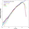 |
Fig. 4 Number counts of galaxies per 0.5 mag per arcmin2 in the U band for the fields in our survey, which have been derived by single-mode photometry. We see that there is very good agreement between our estimates and previous studies (Capak et al. 2004; Eliche-Moral et al. 2006; Rovilos et al. 2009; Grazian et al. 2009). |
In Table 2 we present the number counts of galaxies (in 0.5 mag bins) for the three fields in our dataset. The galaxy counts were obtained by detecting the sources directly in the G and U bands. Thus, the magnitude in this case was not calculated using Eq. (4), but by applying the same photometric method as for the R band (i.e., Eqs. (1)−(3) for each band). In Fig. 3 we show the counts in the G band and in Fig. 4 the counts in the U band for the whole galaxy sample. In both figures we see that our galaxy counts are consistent with all previous studies, which is a further indication of the robustness of our photometry. In particular for the G band, we compared our results to the work of Shim et al. (2006) that presented deep G counts using the MegaCam on the CFHT. Their catalog is 50% complete down to G = 26.5, but they only present number counts down to G = 25.0. We see that their data are fairly consistent with our curves, considering field-to-field variations. In the U band we compared our counts with those of Capak et al. (2004), Eliche-Moral et al. (2006), Rovilos et al. (2009), and Grazian et al. (2009). Again, our results are in agreement with all the aforementioned surveys, and the field-to-field variations are relatively small at U ≥ 22.0.
 |
Fig. 5 U − G vs. G − R diagram that was used for the selection of the LBG candidates in the field Q1623, that is the deepest of the three. Red lines indicate the selection color locus. Green symbols indicate sources with spectroscopic redshift zsp ≤ 2.7, and blue symbols show LBGs with zsp > 2.7 (Reddy, priv. comm.). Vertical arrows indicate upper limits in the U band. Black points indicate all sources detected in the field with R ≤ 25.0. Sources with spectroscopic redshift have magnitudes R ≤ 25.5. |
4. LBG candidates’ selection criteria
For selecting LBG candidates at redshift z ~ 3, we use the (U − G) vs. (G − R) color–color selection technique that was introduced by Steidel and collaborators. The LBC filters are slightly different from the filter set used by Steidel and for this reason we modified their color selection to fit our filter set using the relation found in Giallongo et al. (2008). This relation has been checked with synthetic color predictions derived from galaxy spectral synthesis models (Bruzual & Charlot 2003). The optimized cuts for our filter set are  We verified our cuts by plotting the sources with known spectroscopic redshift on the color–color diagram. As expected most of the sources with redshift above 2.7 are within our cuts (80% for Q0933 and 94% for Q1623). On the other hand, those sources that have been selected as photometric LBG candidates at z ~ 3 by Steidel et al. (2003) but then turned out to be at lower redshift are mostly outside our cuts (93% for Q1623 and 62.5% for Q0933). This means that our sample suffers less from contamination by lower redshift galaxies than previous studies, and this is mainly due to our deeper images in the U band that allow us to select our LBG candidates better. In Fig. 5 we show the (U − G) vs. (G − R) diagram for the Q1623 field, which is the deepest area studied in this work, along with the sources with spectroscopic redshifts (Reddy, priv. comm.). In the COSMOS field, where only photometric redshifts are available in this redshift range (Lilly et al. 2007), we find that for magnitudes 22.0 < R < 24.5, 76% of the sources with 2.7 ≤ zphot ≤ 3.4 are within our cuts (thus selected as LBG candidates), while only 8% of sources with lower photometric redshift (2.0 < zphot < 2.7) contaminate our sample.
The choice of adapting our color cuts to the Steidel criterion was made to be able to compare our results directly with previous studies. In fact, according to stellar models (Pickles 1998; Gunn & Stryker 1983), in the lower right region delimited by our cuts, there could be contamination by stellar sources that are difficult to purge at faint magnitudes by morphological criteria alone. By strictly following the limits of the synthetic SEDs for LBGs, the color cut should be steeper, leaving out the stellar locus. But such a cut would also leave out several spectroscopically confirmed LBGs that do not follow the model tracks exactly.
 |
Fig. 6 Number counts of LBG candidates in each field of our survey. The dashed lines represent the number counts of the candidates in the relative fields obtained by Steidel’s catalogs (Steidel et al. 2003). The total counts for all Steidel fields were obtained from Table 2 of Reddy et al. (2008), and they are not corrected for contamination or completeness. The magenta curve shows the weighted mean of the total raw LBG counts in this survey. |
 |
Fig. 7 Weighted mean of the uncorrected LBG counts of our survey. The LBG count numbers by Nonino et al. (2009) and Reddy et al. (2008) are not corrected for contamination. The count numbers by Ly et al. (2011) and Capak et al. (2004) are corrected for star contamination. We also show the original number-count curve by Steidel et al. (1999), corrected for intelopers. Among recent works, we present the curve for field-1 by van der Burg et al. (2010) and the surface density presented by Bian et al. (2013) for the Bo |
In Fig. 6 we show the results of the LBG counts derived with our selection criteria in the three different fields and show how these counts compare to the Steidel results (Steidel et al. 2003), in the fields we have in common. In the Q0933 field, our results are in very good agreement with the Steidel counts at bright magnitudes and begin to diverge at around R ~ 25, where our curve becomes steeper, since we find more LBG candidates. This is because our 10σ magnitude limit is deeper than their adopted 3σR-band magnitude cut, thus our detections suffer less by incompleteness at the faint end. The LBG counts in Q0933 alone, as already noted by Steidel et al. (2003), are steeper than the average counts derived after combining the entire dataset. In Q1623, a field that is very close to the galactic plane, it is rather difficult to exclude all stars. In fact, we see that the Steidel counts for this field are heavily contaminated by stars at all magnitudes brighter than 24.5. Our morphological criterion for separating extended sources seems to produce acceptable results down to a magnitude of 23.0 in the R band. In the brightest magnitude bin (22.0−23.0) however, ours too is contaminated by stars, and this bump is visible in our combined-counts curve. At the faint end, our LBG counts for Q1623 are still a lot steeper than the results presented by Steidel. This is our deepest field in the R band, reaching one magnitude fainter than previous studies. The counts in the COSMOS field are consistent with our results in the other two fields. Our combined-counts curve is consistent with previous studies in the bright end and becomes steeper for R > 24.0.
In Fig. 7 we show the counts of our LBG candidates in the R band and compare them to other works. Our curve is higher than the original Steidel counts (Steidel et al. 1999), but this is a common trend in all subsequent similar works. Actually, Capak et al. (2004) used a slightly different filter set (U − B vs. B − R) to select the U dropouts, and their R counts, after removing the stars, reach a magnitude limit of <26.0, which is almost 0.5 mag brighter than our deepest R-band image. This is also true for their U-band images, since their 5σ limit corresponds to our 10σ magnitude limit. Thus the images used by Capak et al. (2004), are 0.5 mag deeper than Steidel’s and are consistent with our counts at the bright end. At the faint end, they are more consistent with Reddy et al. (2008), but that their R images are 0.5 mag brighter than our dataset could explain this discrepancy. In fact, recent works presented by Nonino et al. (2009) and Ly et al. (2011), are in good agreement with our results. Although consistent with the latter studies at the faint end, the counts presented by van der Burg et al. (2010) appear significantly lower with respect to all previous surveys for R magnitude brighter than 24.0. This could be due to the different wavelength coverage of the U filter adopted in the CFHT survey, which is offset to redder wavelengths with respect to standard U filters. Consequently, the redshift selection function could be centered at a slightly higher redshift than previous studies, where there are fewer objects. According to van der Burg et al. (2010), the estimated mean redshift for their U dropouts is ⟨ z ⟩ = 3.1 ± 0.1, while for the LBC filter set, it is ⟨ z ⟩ = 2.9. The most recent survey, presented by Bian et al. (2013), also shows counts that at the bright end are systematically lower than the work of Reddy et al. (2008). As seen in Fig. 7, our counts are between the two curves reported by Reddy et al. (2008) and Bian et al. (2013) in the bright magnitude range, and this could either be due to cosmic variance or to slight differences in the color criteria used in each survey.
Counts of LBG candidates for each field in the R band.
In Table 3 we present the number counts for our LBG candidates in bins of 0.5 mag. The last column presents the average number counts per arcmin2, weighted with the area and corrected for completeness (see Sect. 5). For magnitudes fainter than 25.5, each field contributes to this average, up to the magnitude limit where relative completeness is >80%.
The total surface density of LBG candidates for each field in the magnitude range 23.0 < R < 25.5, weighted by area, is 3.23 sources/arcmin2 in COSMOS, 3.73 sources/arcmin2 in Q0933, and 2.49 sources/arcmin2 in Q1623. The average number for our total survey is 3.15 ± 0.62 sources per arcmin2, which leads to a cosmic variance of ~20%. Using the original catalogs presented by Steidel et al. (2003), in the fields we have in common, we find a surface density of LBG candidates of 2.5 sources/arcmin2 for Q0933 and 1.8 sources/arcmin2 for Q1623. We obtain this result without taking into consideration subsequent adjustments for completeness and interlopers based on the spectroscopic follow-up. According to Steidel et al. (2003), the overall surface density in their survey is 1.8 LBG candidates per arcmin2, uncorrected for completeness, which is lower than the estimate based on our analysis by 40%. This could be explained by the fact that this magnitude (R = 25.5) corresponds to their 3σ limit, so their survey could be less complete. In more recent surveys, Rovilos et al. (2009) find 2.3 sources per arcmin2 and Rafelski et al. (2009) find 3.7 ± 0.6 (LRD field) and 4.3 ± 0.2 (KDF field) for V < 26.0, which corresponds to our magnitude limit of R < 25.5. For fainter magnitudes, Sawicki & Thompson (2006) find 8.8 LBG candidates/arcmin2 (50% completeness at R ≈ 27.0) and Nonino et al. (2009) report a surface density of 7.3 arcmin-2 at a similar magnitude limit, although they are already >50% incomplete by R = 26.0. In our deepest field, Q1623, where we also have 50% completeness at R = 27.0, we find 10.8 LBG candidates/arcmin2, based on the raw number counts. Although it is difficult to directly compare with previous surveys, due to different completeness fractions at that magnitude limit, we see that our surface density is consistent with previous surveys at faint magnitudes, when taking the cosmic variance into account.
In Appendix A we provide the LBG candidate catalog in each field, down to the 50% completeness magnitude limit in the R band. The magnitudes presented in these catalogs have been calculated using the R band as the detection image, and for the other two bands (G and U), we report the corrected aperture magnitudes, derived in dual-mode photometry according to Eq. (4). For each magnitude we also report the associated error. Negative magnitude values in the G and U bands, indicate upper limits at 1σ. For the R band, where the sources were detected, we also present a signal-to-noise ratio estimate, the measured FWHM in pixels, and the morphological class attributed to the source by SExtractor, with values closer to zero indicating an extended morphology.
5. Completeness and interlopers
To estimate the completeness of our sample, we use a set of simulations. First, we select stellar sources with magnitudes in the range of 23.0 < R < 24.0 and FWHM < FWHMcut (see Sect. 3), and we stack them to create a point spread function (PSF) template. We then randomly place 1000 of these stacked PSFs at different R magnitudes in our images. We then repeat the detection procedure and check the percentage of sources recovered by our method. We apply the same method, also using galaxy profiles. To create the galaxy profiles, we selected LBG candidates in three different magnitude bins centered at 24.0, 25.0, and 26.0, after visual inspection for contamination by neighboring sources. We made three stacked images, one for each magnitude bin, which we then randomly placed and recovered, as described above. We show an example of these simulations in field Q1623 and how the various completeness curves compare in Fig. 8. We see that using a PSF, which is created by stars, gives very similar results to the profiles created by stacking faint galaxies (R = 26.0) and they correspond to our lower limit in the completeness curves. By using profiles based on brighter galaxies (R = 25.0 and 24.0), the corrections are larger, since brighter galaxies are more extended and this could compromise the detection efficiency (Cohen et al. 2003). Since the stellar PSF gives us the lower limit for the completeness curve, and it is also very similar to the faintest galaxy curve, we decided to repeat the simulations using only stellar PSFs for the other two fields, as a conservative approach.
 |
Fig. 8 Completeness corrections derived from simulations in Q1623, which is the deepest of our fields, using PSFs created by stacking real stellar and extended sources in different bins of magnitude. |
Another concern in our survey is the fraction of lower redshift interlopers contaminating the LBG candidate selection. To quantify the number of interlopers in our sample, we use the spectroscopic data available in COSMOS for z < 1.5 and in the Q1623 field for z > 1.5. To perform simulations in the magnitude range 25.0 ≤ R ≤ 27.0 we selected fairly bright sources (23.0 < R < 24.50) for a total of 240 objects with known redshift. The sample is divided into redshift bins of 0.2, and the number of real sources in our spectroscopic catalogs has been normalized according to the redshift distribution obtained at faint magnitudes (in bins of 0.5 mag) by the Millennium simulation (Kitzbichler & White 2007).
This technique allows us to reproduce the actual redshift distributions in different magnitude ranges starting from our spectroscopic catalogs which are limited at bright R-band magnitudes. Starting from the observed UGR photometry of the spectroscopic catalog, renormalized in number, we extrapolate the photometry to fainter magnitudes, reproducing the observed magnitude-error relations for each band. All sources with spectroscopic redshift used in the input catalog are correctly allocated in the color–color diagram; thus, all sources inside the color–color selection locus are LBGs at z ≈ 3, and all sources outside have lower redshifts. From the output catalog we can assess the number of sources that are detected as bright LBG candidates but at fainter magnitudes have moved outside the color–color selection locus, because of the photometric error.
We can also estimate the number of sources that were outside the color–color locus and are now detected as spurious LBG candidates. To repeat the simulations for the brighter magnitude range of 24.0 ≤ R ≤ 25.0, the same method was adopted after restricting the input catalog of sources with known redshift to 23.0 ≤ R < 24.0 (155 objects). We see that the maximum of the net effect of the scatter for sources going in and out of the color locus (net contamination) is reached around R = 26.0, where we have ~21% more sources with z < 2.7 entering the color–color selection area. For fainter magnitudes, according to the redshift distributions, there are less sources of lower redshift that can end up in the color–color locus of LBGs because of photometric error, so it is reasonable that the percentage of contamination is actually lower. Our results are in accordance with the contamination reported by Hildebrandt et al. (2007), who find a 20% contamination in the magnitude range 22.0 < R < 26.0.
Completeness in the R band for each field and total “net contamination” fraction.
 |
Fig. 9 Detection efficiencies in the R band derived by simulations in all 3 fields using PSFs created by stacking stellar sources down to 24.0 in the R band. The black curve indicates the percentage of the “net contamination” fraction we expect in the total sample as a function of magnitude. |
To quantify the contamination by stars, we select all stars in the COSMOS field based on a BzK selection and on spectroscopic data (using publicly available photometry). After cross-correlating this catalog to the catalog of our LBG candidates in COSMOS, we only find ten sources in common out of ~4000 candidates, which are evenly distributed in the magnitude range 23.0 < R < 26.3. Thus, our contamination by stars is negligible (0.25%).
In Table 4 we present the completeness calculated for each field, in bins of 0.25 mag, as well as the “net contamination” fraction for the same magnitude bins, after a spline fitting of the values obtained through simulations. In Fig. 9 we show the relative plot with the detection efficiencies, where the “net contamination” fraction is also presented, although we do not correct our number counts for this effect. We see that down to a magnitude of R = 25.5, completeness is above 99.5% (practically complete) for all our fields. For Q0933, completeness rapidly decreases after this limit, reaching 50% at a magnitude of R = 26.1, making it the shallowest of the three fields. The COSMOS field follows, since it is 50% complete at R = 26.5, and Q1623 reaches this limit at R = 27.0, leading to the deepest in our survey. Actually, Q1623 is the field with the deepest photometry in all three bands, as shown in Table 1, and with the greatest number of spectroscopically confirmed LBGs, thus it is ideal for exploring the limits of our color selection.
 |
Fig. 10 Weighted average for the LBG counts, after correcting for completeness. The average is based on all 3 fields until R = 25.5 and, for fainter magnitudes, only the two deepest fields are considered (Q1623 and COSMOS), with a conservative cut made at ~80% completeness. We also show the double power law fit of this curve and the derived values for α = 1.04 and β = 0.13, m∗ = 25.01 and log N∗ = 0.39, where N is the number of galaxies per arcmin2 per 0.5 mag bins. The dotted lines show the upper and lower limit curves. |
Based on these curves we calculate a weighted average for the counts of LBG candidates in all our fields, corrected for completeness. To account for the different depths of our fields, we used the counts of the entire dataset up to mag = 25.5 in R band. After this magnitude limit, completeness for the Q0933 field is flattening and the corrections become increasingly large (completeness ~95% already at R = 25.6), so we only use the counts of the other two fields, Q1623 and COSMOS, for the faint bins of our survey (25.5 ≤ R < 26.2). The last bins (26.2 ≤ R ≤ 27.0) are entirely computed using only Q1623. We then fit this curve with a double power law, in order to derive the slope. To be conservative, we apply the fit only down to R = 26.6, where completeness is >80%. After this magnitude limit, we see that the curve is flattening even though it is corrected for completeness. The double power law is described by the following formula:  (8)In Fig. 10 we show both the curve corresponding to the weighted average corrected for completeness and the double power law fit. The two slopes derived from this fit are α = 1.04 and β = 0.13, with the break located at m∗ = 25.01 and log N∗ = 0.39, where N is the number of galaxies per arcmin2 per 0.5 mag bins. The fit for the lower limit curve at 1σ is α = 1.16, β = 0.20, m∗ = 24.8, log N∗ = 0.25, and for the upper limit curve the fit corresponds to α = 0.94, β = 0.06, m∗ = 25.2, and log N∗ = 0.51. There are no records of similar analysis in the literature, so we cannot directly compare our results with previous studies.
6. Discussion and summary
We presented a deep multiband imaging survey with the LBC, covering an area of ~1500 arcmin2. We reobserved two fields used in Steidel’s original survey (Q0933 and Q1623, Steidel et al. 2003), where we obtained deeper R- and U-band imaging. A similar dataset was also obtained for the COSMOS field, where there is available public multiband photometry as well as photometric and spectroscopic redshifts. We reached 50% completeness at R magnitude of 27.0, 26.1, and 26.5 for Q1623, Q0933, and COSMOS, respectively. The 1σ magnitude limit in the U band is between 28.5−28.7 on the whole area, which is a good compromise between depth and total area, compared to other surveys, so far. A significant advantage of our sample is that the U band is much deeper than previous samples. For a limiting magnitude of R = 27.0 (50% completeness) in our deepest field and an average magnitude in the U band of 28.6 at 1σ (2 × FWHM apertures), this is the only survey with a wide dynamic range in the color selection, allowing us to robustly select LBG candidates with minimum contamination. In comparison, the CFHT survey (van der Burg et al. 2010), although reaching 27.9 in the R band (5σ for point sources), is shallower in the U band than ours. At the bright end we are fairly consistent with the new survey presented by Bian et al. (2013) in the NOAO Botes Field, but the two surveys start diverging after R > 24.0, since the latter one is two magnitudes shallower than our survey, although it is covering a much larger area (~9 sq. deg).
Comparing our candidates with existing spectroscopy in the Steidel fields, where spectroscopic redshifts are available, we show that the deeper U-band dataset allows us to better separate confirmed LBGs at z ≈ 3 from lower redshift interlopers. Although we have less contamination by low-redshift sources, we can see in Fig. 8 that the slope of our LBG counts is actually steeper than previous studies, suggesting that there are more LBGs at faint magnitudes. The slopes we derived are α = 1.04 at the bright end and β = 0.13 at the faint end, with a break at m∗ = 25.01 and log N∗ = 0.39. We find an average surface density of 3.15 LBG candidates per arcmin2 down to R = 25.5, which rises to 10.8 LBG candidates per arcmin2 when we go as faint as R = 27.0.
This dataset will be the benchmark for a series of future analysis. We intend to obtain spectroscopic follow-up for our brightest candidates, to verify our contamination by interlopers. This extended spectroscopic sample, complemented with deep ULTRA-VISTA images in the COSMOS field will be used for determining stellar masses, ages, and dust content of faint LBGs at z ≈ 3. It will also be possible to measure the UV slope of galaxies in the wavelength range from 1500 Å to 3000 Å (rest frame), using a method similar to the one we applied at z ≈ 4 (Castellano et al. 2012). In addition, based on this sample, we will update our measurement of the escape fraction of Lyα continuum, attributed to LBGs at this redshift, in an effort to understand their contribution to the reionization of the Universe.
Acknowledgments
K.B. would like to thank N. Reddy for providing redshifts for the sources in the Q1623 field, which are not publicly available. We would also like to thank the referee for useful comments that significantly improved the quality of this work.
References
- Bertin, E., & Arnouts, S. 1996, A&AS, 117, 393 [NASA ADS] [CrossRef] [EDP Sciences] [Google Scholar]
- Bian, F., Fan, X., Jiang, L., et al. 2013, ApJ, 774, 28 [NASA ADS] [CrossRef] [Google Scholar]
- Boutsia, K., Grazian, A., Giallongo, E., et al. 2011, ApJ, 736, 41 [NASA ADS] [CrossRef] [Google Scholar]
- Bruzual, G., & Charlot, S. 2003, MNRAS, 344, 1000 [NASA ADS] [CrossRef] [Google Scholar]
- Capak, P., Cowie, L. L., Hu, E. M., et al. 2004, AJ, 127, 180 [NASA ADS] [CrossRef] [Google Scholar]
- Castellano, M., Fontana, A., Grazian, A., et al. 2012, A&A, 540, A39 [NASA ADS] [CrossRef] [EDP Sciences] [Google Scholar]
- Cohen, S. H., Windhorst, R. A., Odewahn, S. C., Chiarenza, C. A., & Driver, S. P. 2003, AJ, 125, 1762 [NASA ADS] [CrossRef] [Google Scholar]
- Dickinson, M., Stern, D., Giavalisco, M., et al. 2004, ApJ, 600, L99 [NASA ADS] [CrossRef] [Google Scholar]
- Eliche-Moral, M. C., Balcells, M., Prieto, M., et al. 2006, ApJ, 639, 644 [NASA ADS] [CrossRef] [Google Scholar]
- Giallongo, E., Ragazzoni, R., Grazian, A., et al. 2008, A&A, 482, 349 [NASA ADS] [CrossRef] [EDP Sciences] [Google Scholar]
- Giavalisco, M. 2002, ARA&A, 40, 579 [NASA ADS] [CrossRef] [Google Scholar]
- Grazian, A., Menci, N., Giallongo, E., et al. 2009, A&A, 505, 1041 [NASA ADS] [CrossRef] [EDP Sciences] [Google Scholar]
- Gunn, J. E., & Stryker, L. L. 1983, ApJS, 52, 121 [NASA ADS] [CrossRef] [Google Scholar]
- Hildebrandt, H., Pielorz, J., Erben, T., et al. 2007, A&A, 462, 865 [NASA ADS] [CrossRef] [EDP Sciences] [Google Scholar]
- Iwata, I., Ohta, K., Tamura, N., et al. 2007, MNRAS, 376, 1557 [NASA ADS] [CrossRef] [Google Scholar]
- Kitzbichler, M. G., & White, S. D. M. 2007, MNRAS, 376, 2 [NASA ADS] [CrossRef] [Google Scholar]
- Le Fèvre, O., Paltani, S., Arnouts, S., et al. 2005, Nature, 437, 519 [NASA ADS] [CrossRef] [Google Scholar]
- Lilly, S. J., Le Fèvre, O., Renzini, A., et al. 2007, ApJS, 172, 70 [NASA ADS] [CrossRef] [Google Scholar]
- Lilly, S. J., Le Brun, V., Maier, C., et al. 2009, ApJS, 184, 218 [Google Scholar]
- Ly, C., Malkan, M. A., Hayashi, M., et al. 2011, ApJ, 735, 91 [NASA ADS] [CrossRef] [Google Scholar]
- Madau, P. 1995, ApJ, 441, 18 [NASA ADS] [CrossRef] [Google Scholar]
- Metcalfe, N., Shanks, T., Campos, A., McCracken, H. J., & Fong, R. 2001, MNRAS, 323, 795 [NASA ADS] [CrossRef] [Google Scholar]
- Nonino, M., Dickinson, M., Rosati, P., et al. 2009, ApJS, 183, 244 [NASA ADS] [CrossRef] [Google Scholar]
- Pickles, A. J. 1998, PASP, 110, 863 [CrossRef] [Google Scholar]
- Rafelski, M., Wolfe, A. M., Cooke, J., et al. 2009, ApJ, 703, 2033 [NASA ADS] [CrossRef] [Google Scholar]
- Reddy, N. A., Steidel, C. C., Pettini, M., et al. 2008, ApJS, 175, 48 [NASA ADS] [CrossRef] [Google Scholar]
- Rovilos, E., Burwitz, V., Szokoly, G., et al. 2009, A&A, 507, 195 [NASA ADS] [CrossRef] [EDP Sciences] [Google Scholar]
- Sawicki, M., & Thompson, D. 2005, ApJ, 635, 100 [NASA ADS] [CrossRef] [Google Scholar]
- Sawicki, M., & Thompson, D. 2006, ApJ, 648, 299 [NASA ADS] [CrossRef] [Google Scholar]
- Scoville, N., Aussel, H., Brusa, M., et al. 2007, ApJS, 172, 1 [NASA ADS] [CrossRef] [Google Scholar]
- Shim, H., Im, M., Pak, S., et al. 2006, ApJS, 164, 435 [NASA ADS] [CrossRef] [Google Scholar]
- Steidel, C. C., Giavalisco, M., Pettini, M., Dickinson, M., & Adelberger, K. L. 1996, ApJ, 462, L17 [NASA ADS] [CrossRef] [Google Scholar]
- Steidel, C. C., Adelberger, K. L., Giavalisco, M., Dickinson, M., & Pettini, M. 1999, ApJ, 519, 1 [NASA ADS] [CrossRef] [Google Scholar]
- Steidel, C. C., Adelberger, K. L., Shapley, A. E., et al. 2003, ApJ, 592, 728 [NASA ADS] [CrossRef] [Google Scholar]
- Steidel, C. C., Shapley, A. E., Pettini, M., et al. 2004, ApJ, 604, 534 [NASA ADS] [CrossRef] [Google Scholar]
- van der Burg, R. F. J., Hildebrandt, H., & Erben, T. 2010, A&A, 523, A74 [NASA ADS] [CrossRef] [EDP Sciences] [Google Scholar]
- Yan, H., & Windhorst, R. A. 2004, ApJ, 612, L93 [NASA ADS] [CrossRef] [Google Scholar]
Appendix A: detailed catalogs for the LBG candidates
LBG candidates in Q1623 – sample.
LBG candidates in COSMOS – sample.
LBG candidates in Q0933 – sample.
All Tables
Completeness in the R band for each field and total “net contamination” fraction.
All Figures
|
Fig. 1 Transmission of LBC filters used in our survey. These curves include the telescope and instrument response but not the atmospheric response, since the data have been obtained during several observing runs with varying weather conditions. For the U and R filters there are two curves that represent the different filters. The blue solid line represents Uspecial and the blue dashed line represents Ubessel. The red solid line represents R-Sloan in the red channel, and the dashed line is the transmission of the R-Sloan filter in the blue channel. There is only one G-Sloan filter on LBC-Blue. |
| In the text | |
|
Fig. 2 Galaxy counts (number of sources per 0.5 mag per arcmin2) in the R band derived from our analysis separately in each field. There is good agreement with previous estimates (Metcalfe et al. 2001; Capak et al. 2004), which is a strong indication of the robustness of our photometry. |
| In the text | |
|
Fig. 3 Galaxy counts in the G band for each of our fields separately. The magnitudes of the galaxies for this plot were derived by single-mode photometry, detecting sources directly in the G-band images. Although we see some scatter in the bright end, there is overall agreement when compared to the literature (Shim et al. 2006). |
| In the text | |
|
Fig. 4 Number counts of galaxies per 0.5 mag per arcmin2 in the U band for the fields in our survey, which have been derived by single-mode photometry. We see that there is very good agreement between our estimates and previous studies (Capak et al. 2004; Eliche-Moral et al. 2006; Rovilos et al. 2009; Grazian et al. 2009). |
| In the text | |
|
Fig. 5 U − G vs. G − R diagram that was used for the selection of the LBG candidates in the field Q1623, that is the deepest of the three. Red lines indicate the selection color locus. Green symbols indicate sources with spectroscopic redshift zsp ≤ 2.7, and blue symbols show LBGs with zsp > 2.7 (Reddy, priv. comm.). Vertical arrows indicate upper limits in the U band. Black points indicate all sources detected in the field with R ≤ 25.0. Sources with spectroscopic redshift have magnitudes R ≤ 25.5. |
| In the text | |
|
Fig. 6 Number counts of LBG candidates in each field of our survey. The dashed lines represent the number counts of the candidates in the relative fields obtained by Steidel’s catalogs (Steidel et al. 2003). The total counts for all Steidel fields were obtained from Table 2 of Reddy et al. (2008), and they are not corrected for contamination or completeness. The magenta curve shows the weighted mean of the total raw LBG counts in this survey. |
| In the text | |
|
Fig. 7 Weighted mean of the uncorrected LBG counts of our survey. The LBG count numbers by Nonino et al. (2009) and Reddy et al. (2008) are not corrected for contamination. The count numbers by Ly et al. (2011) and Capak et al. (2004) are corrected for star contamination. We also show the original number-count curve by Steidel et al. (1999), corrected for intelopers. Among recent works, we present the curve for field-1 by van der Burg et al. (2010) and the surface density presented by Bian et al. (2013) for the Bo |
| In the text | |
|
Fig. 8 Completeness corrections derived from simulations in Q1623, which is the deepest of our fields, using PSFs created by stacking real stellar and extended sources in different bins of magnitude. |
| In the text | |
|
Fig. 9 Detection efficiencies in the R band derived by simulations in all 3 fields using PSFs created by stacking stellar sources down to 24.0 in the R band. The black curve indicates the percentage of the “net contamination” fraction we expect in the total sample as a function of magnitude. |
| In the text | |
|
Fig. 10 Weighted average for the LBG counts, after correcting for completeness. The average is based on all 3 fields until R = 25.5 and, for fainter magnitudes, only the two deepest fields are considered (Q1623 and COSMOS), with a conservative cut made at ~80% completeness. We also show the double power law fit of this curve and the derived values for α = 1.04 and β = 0.13, m∗ = 25.01 and log N∗ = 0.39, where N is the number of galaxies per arcmin2 per 0.5 mag bins. The dotted lines show the upper and lower limit curves. |
| In the text | |
Current usage metrics show cumulative count of Article Views (full-text article views including HTML views, PDF and ePub downloads, according to the available data) and Abstracts Views on Vision4Press platform.
Data correspond to usage on the plateform after 2015. The current usage metrics is available 48-96 hours after online publication and is updated daily on week days.
Initial download of the metrics may take a while.