| Issue |
A&A
Volume 563, March 2014
|
|
|---|---|---|
| Article Number | A69 | |
| Number of page(s) | 17 | |
| Section | Interstellar and circumstellar matter | |
| DOI | https://doi.org/10.1051/0004-6361/201321151 | |
| Published online | 14 March 2014 | |
Ionization rates in the heliosheath and in astrosheaths
Spatial dependence and dynamical relevance⋆
1
Institut für Theoretische Physik IV, Ruhr-Universität Bochum,
44780
Bochum, Germany
e-mail: kls@tp4.rub.de; hf@tp4.rub.de
2
Argelander Institut, Universität Bonn,
53121
Bonn,
Germany
e-mail:
hfahr@astro.uni-bonn.de
3
Polish Space Science Center, Bartycka 18A, 00-716
Warsaw,
Poland
e-mail:
bzowski@cbk.waw.pl
4
Centre for Space Research, North-West University,
2520
Potchefstroom, South
Africa
e-mail:
Stefan.Ferreira@nwu.ac.za
Received:
22
January
2013
Accepted:
5
December
2013
Context. In the heliosphere, especially in the inner heliosheath, mass-, momentum-, and energy-loading induced by the ionization of neutral interstellar species plays an important, but for some species, especially helium, an underestimated role.
Aims. We discuss the implementation of charge exchange and electron impact processes for interstellar neutral hydrogen and helium and their implications for the subsequent modeling. We especially emphasize the importance of electron impact and a more sophisticated numerical treatment of the charge exchange reactions. Moreover, we discuss the nonresonant charge exchange effects.
Methods. We discuss rate coefficients and revise the influence of the cross-sections in the (magneto-)hydrodynamic equations for different reactions and also their representation in the collision integrals.
Results. Electron impact is in some regions of the heliosphere, particularly in the heliotail, more effective than charge exchange, and the ionization of neutral interstellar helium contributes about 40% to the mass- and momentum-loading in the heliosheath. The charge exchange cross-sections need to be modeled with higher accuracy, especially in view of the latest developments made in describing them.
Conclusions. The ionization of helium and the electron impact ionization of hydrogen need to be taken into account in modeling the heliosheath and, in general, astrosheaths. Moreover, the charge exchange cross-sections need to be handled in a more sophisticated way, either by developing better analytic approximations or by numerically solving the collision integrals.
Key words: Sun: heliosphere / stars: winds, outflows / hydrodynamics / atomic processes
Appendices are available in electronic form at http://www.aanda.org
© ESO, 2014
1. Introduction
1.1. General aspects
It is well-known that not only the interstellar plasma, but also the interstellar neutral gas influences the large-scale structure of the heliosphere (Baranov & Malama 1993; Scherer & Ferreira 2005; Müller et al. 2008; Zank et al. 2013). This influence is a consequence of the coupling of the neutral gas (consisting mainly of hydrogen and helium) to the solar wind plasma (mainly protons with a small contribution of α particles (He2+)) via charge exchange, photoionization, and electron impact processes. Elastic collisions and Coulomb scattering have been discussed in Williams et al. (1997).
In selfconsistent models of heliospheric dynamics, so far only the influence of neutral hydrogen is considered by taking into account its charge exchange with solar wind protons and its ionization by the solar radiation (e.g. Fahr & Ruciński 2001; Pogorelov et al. 2009; Alouani-Bibi et al. 2011, and references therein). The dynamical relevance of both the electron impact ionization of hydrogen, although recognized by Malama et al. (2006), and the photoionization of helium, although recognized as being filtrated in the inner heliosheath (Rucinski & Fahr 1989; Cummings et al. 2002), have not yet been explored in detail. Only Malama et al. (2006) included helium selfconsistently in the heliospheric modeling and discussed the additional ram pressure generated by the charged helium ions.
In recent years the discussion has rather concentrated on the correct cross-section for the charge exchange between a proton and a hydrogen atom. While it has been demonstrated by Williams et al. (1997) that the modeling results regarding the large-scale structure (location of the termination shock and heliopause) are insensitive to the alternative cross-sections given by Fite et al. (1962) and Maher & Tinsley (1977), it was revealed that it is important for the neutral gas (shape of the hydrogen wall and densities inside the termination shock, see, e.g. Baranov et al. 1998; Heerikhuisen et al. 2006). Subsequently, the significance of the revised cross-sections by Lindsay & Stebbings (2005) has first been recognized by Fahr et al. (2007) and has been discussed in more detail in the context of global heliospheric modeling by Müller et al. (2008), Bzowski et al. (2008), and Izmodenov et al. (2008).
It has also been recognized that electron impact ionization is not only important for the neutral gas distribution (e.g., Rucinski & Fahr 1989; Möbius et al. 2004; Izmodenov 2007) but to some extent also for the large-scale structure of the heliosphere (Fahr et al. 2000; Scherer & Ferreira 2005; Malama et al. 2006). However, these studies contain neither a comparison of the electron impact ionization rates with those of the other two processes, nor a systematic analysis of their dynamical influence.
In addition to addressing the first of these problems here, we show that not only the ionization of neutral hydrogen influences the dynamics in the heliosphere, but that neutral helium must also be expected to play a role. Furthermore, we discuss charge exchange reactions of hydrogen and helium in view of their relevance to astrospheres, particularly to astrosheaths. In astrospheres the relative speed between a stellar wind and the flow of neutrals from the interstellar medium can be up to an order of magnitude higher than in the solar case, see for example the M-dwarf V-Peg 374 (Vidotto et al. 2011) or for hot stars (e.g. Arthur 2012).
Before quantitatively addressing these topics, we briefly indicate other heliospheric and astrophysical applications for which the ionization rates studied here also are of interest.
The charge exchange process has recently gained more interest because it is responsible for the outer-heliospheric production of energetic neutral atoms (see Fahr et al. 2007,for a comprehensive review) that are presently observed with the IBEX mission (McComas et al. 2009, 2012; Funsten et al. 2009; Dayeh et al. 2012). In this context, Grzedzielski et al. (2010) investigated the distribution of different pickup-ion (PUI) species, which are products of ionization processes in the inner heliosheath, and Borovikov et al. (2011) discussed their influence on the plasma state of the inner heliosheath. Furthermore, Aleksashov et al. (2004) began to explore the influence of charge exchange of hydrogen atoms with solar wind protons and their impact on the structure of the heliotail. The charge exchange processes of heavier elements were studied in connection with the X-ray production in the inner heliosphere (Koutroumpa et al. 2009), while these processes in the local interstellar medium are discussed by Provornikova et al. (2012).
Astrophysical scenarios for which the use of correct ionization rates is crucial (Nekrasov 2012) comprise the X-ray emission from galaxies (Wang & Liu 2012), from the interstellar medium (de Avillez & Breitschwerdt 2012), and from hot stars (Pollock 2012), the influence of neutral atoms on astrophysical shocks (Blasi et al. 2012; Ohira 2012), and the jets of active galactic nuclei (Gerbig & Schlickeiser 2007).
We here concentrate on the relative importance of the different ionization processes for the heliosheath and for astrosheaths, that is for the regions between the solar or stellar wind termination shock/s and the helio- or astropauses, then to later incorporate into corresponding selfconsistent (magneto-)hydrodynamic ((M)HD) modeling with the BoPo (Scherer & Ferreira 2005) and the CRONOS code (see Wiengarten et al. 2013, for an application and references therein). We demonstrate the significance and dynamical relevance of electron impact ionization of hydrogen and of helium in the entire heliosphere by employing the well-established heliospheric model by Fahr et al. (2000) and Scherer & Ferreira (2005). The model includes for our computation charge exchange between neutral and ionized hydrogen, electron impact of hydrogen, and photoionization of hydrogen. Considering elastic collisions and Coulomb scattering (Williams et al. 1997) is beyond the scope of this paper.
In Sect. 2 we first give a short introduction to the BoPo code and in Sect. 3 discuss the charge exchange and electron impact cross-sections. In Sect. 4 we describe the interaction terms used in the Euler equations (see Appendix A). In Sect. 5 we then concentrate on the electron impact and its contribution to the interaction terms, which is followed by a discussion of the neutral interstellar helium loss in the inner heliosheath in Sect. 6. Section 7 contains a discussion of the nonresonant charge exchange and its relevance to the outer heliosheath. Finally, we assemble our ideas and critically assess our findings in the concluding Sect. 9.
1.2. Astrospheres and the heliosphere
An astrosphere is a generalization of the heliosphere. The physics is similar, except that for huge astrospheres, such as those around hot stars (Arthur 2012), where a cooling function needs to be included in the region beyond the termination shock. Moreover, for hot stars the Strömgren sphere can be larger then the astrosphere, and thus photoionization can be dominant in the entire astrosphere. Nonetheless, HI regions can exist around hot stars (Arnal 2001; Cichowolski et al. 2003) and thus ionization processes become important. Therefore, an HII region with a variable degree of ionization is a better concept than the classical Strömgren sphere. For example, for the Sun the Strömgren radius RS = 2.2 × 1010 cm (Fahr 1968) is smaller than the solar radius, while its HII region is considerably larger (Lenchek 1964; Ritzerveld 2005; Fahr 2004).
Some cool stars exist like V-Peg 374 (Vidotto et al. 2011) which have stellar wind speeds (≈2000 km s-1) much higher than that of the solar wind. Moreover, for nearby stars the relative speeds between the star and the interstellar medium can differ by factors between 0.2 to 2 compared with the interstellar medium that surrounds the solar system (Wood et al. 2007). For these high relative speeds cross-sections of other processes and different species may become important.
In most of the stellar wind models (e.g. Lamers & Cassinelli 1999) the wind passes through one or more critical points (surfaces) after which it freely expands. This freely expanding continuous blowing wind is physically similar to the solar wind. In an ideal scenario without neutrals and cooling the solutions can simply be scaled from one scenario to the other.
The models for astrospheres are based on MHD equations (see Appendix A) in the same way as for the heliosphere. Because a fleet of spacecraft has been or is exploring the heliosphere by in situ as well as remote measurements, the knowledge of that special astrosphere is much more detailed than that of astrospheres. In the following we make no difference between astrospheres or the heliosphere. All we discuss applies to the heliosphere as well as to astrospheres immersed in partly ionized clouds of interstellar matter.
One interesting feature of some nearby astrospheres is their hydrogen walls, which are built beyond the astropauses by charge exchange between interstellar hydrogen and protons. This feature can be observed in Lyman-α absorption (Wood et al. 2007), which in turn allows one to determine the stellar wind and interstellar parameters of some nearby stars. Because the hydrogen wall is built up in the interstellar medium, where the temperatures are low (<104 K) and because they increase for the heliosphere only by approximately a factor two toward the heliopause, the charge exchange process involved is that between protons and hydrogen as well as some helium reactions, such as He+ + He, He2+ + He, and He+ + He+, which have large cross-sections even at low energies. Owing to the low temperatures, electron impact is not effective, because the involved energies are lower than the ionization energy. Up to now, only hydrogen walls were observed, which, nevertheless, allows for some insights into the structure of nearby astrospheres. Helium walls as a result of helium-proton charge exchange were not found (Müller & Zank 2004b). Nevertheless, some helium-helium reactions with sufficiently large cross-sections (see Fig. 2 or Tables C.1 and C.2) may result in a helium wall.
2. Heliosphere model
For this analysis a detailed model of the heliosphere is not necessarily needed. Nevertheless, we used a snapshot of a dynamic heliosphere model computed with the BoPo-model code (Scherer & Ferreira 2005). This model includes three species, protons, neutral hydrogen, and, from the latter, newly created ions, the pickup protons (PUISH+). The effective temperature distribution, that is the weighted sum of the proton and PUI temperatures of the model, is shown in Fig. 1. The modeled effective temperature nicely reproduces those inferred by IBEX (Livadiotis et al. 2011).
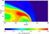 |
Fig. 1 Proton temperature distribution in the dynamic heliosphere (Scherer & Ferreira 2005). Above the solar pole the features of a high-speed stream can be identified. Because of the influence of the PUISH+ the temperature inside the termination shock is a few 105 K, corresponding to thermal energies of up to a few tens of eV. The temperature in the inner heliosheath is 106 K, which was inferred by IBEX (Livadiotis et al. 2011). |
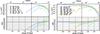 |
Fig. 2 Charge exchange cross-sections as a function of energy per nucleon for protons (left panel), He+-ions, and α-particles (right panel) of the solar wind with interstellar helium and hydrogen. In the upper part of the two panels we show the cross-sections, while the lower parts show the ratio to σcx(H+ + H → H + H+). The black curve in the panels is the reaction H + H+ → H+ + H. As can be seen in the lower panel the reactions He+ + He, He2+ + He, and He2+ + He+ have similar cross-sections as that of H + H+ and thus are important in modeling the dynamics of the large-scale astrospheric structures. Note the different y-axis scales between different panels. |
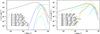 |
Fig. 3 Rate coefficients β(v) = vσ(v)
instead of the cross-sections as in Fig. 2. We
assumed that there is no difference in the relative speeds from the collision
integrals |


The PUISH+ are created by a resonant charge exchange process between a neutral hydrogen
atom and a proton 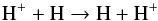 (1)in which an
electron is exchanged between the reaction partners. Because the first reactant is a fast
proton, the neutral hydrogen atom resulting from this interaction is an energetic (fast)
neutral atom (ENA), which here is assumed to leave the heliosphere without further
interaction. The second reactant, a slow interstellar hydrogen atom, becomes ionized and is
immediately picked up by the electromotive force of the heliospheric magnetic field that is
frozen-in in the solar wind. The initial PUIH+ velocity distribution is ring-like with a
maximum of twice the solar wind speed (Vasyliunas &
Siscoe 1976; Isenberg 1995; Gloeckler & Geiss 1998). It very quickly becomes
pitch-angle isotropized, thus transforming into a nearly spherical shell distribution.
(1)in which an
electron is exchanged between the reaction partners. Because the first reactant is a fast
proton, the neutral hydrogen atom resulting from this interaction is an energetic (fast)
neutral atom (ENA), which here is assumed to leave the heliosphere without further
interaction. The second reactant, a slow interstellar hydrogen atom, becomes ionized and is
immediately picked up by the electromotive force of the heliospheric magnetic field that is
frozen-in in the solar wind. The initial PUIH+ velocity distribution is ring-like with a
maximum of twice the solar wind speed (Vasyliunas &
Siscoe 1976; Isenberg 1995; Gloeckler & Geiss 1998). It very quickly becomes
pitch-angle isotropized, thus transforming into a nearly spherical shell distribution.
During this charge exchange process the total ion density does not change, but because of the velocity difference between the proton and neutral hydrogen atom, the solar wind momentum is altered (momentum-loading) as is the energy of the fluid, that is the temperature of the solar wind increases and momentum decreases because it is lost through the escaping ENA (Fahr & Ruciński 1999). This temperature increase was observed by the Voyager spacecraft (Richardson & Wang 2010), while model runs including only a single proton fluid resulted in temperatures of a few hundred Kelvin at the termination shock (for an example see Fig.1 in Fahr et al. 2000). This contrasts with the above-mentioned multifluid and multispecies models with 105 K at the same location (see Fig. 1). The momentum-loading leads to a slowing down of the solar wind, which is indeed observed (Richardson & Wang 2010), in agreement with model attempts (Fahr & Fichtner 1995; Fahr & Ruciński 2001; Fahr 2007; Pogorelov et al. 2004; Alouani-Bibi et al. 2011). Moreover, including neutrals removes the Mach-disks (Baranov et al. 1971; Pauls et al. 1995; Müller et al. 2001) and thus changes the large-scale structure of the astro- or heliosphere and again demonstrates the importance of including charge exchange processes for an adequate description.
The dynamic BoPo model (Fahr et al. 2000;
Scherer & Ferreira 2005) also includes the electron impact
 (2)in
the inner heliosheath, that is the region between the termination shock and the heliopause.
(2)in
the inner heliosheath, that is the region between the termination shock and the heliopause.
The photoionization inside the termination shock is also included. This leads not only to the above-described momentum- and energy-loading but, also to a mass-loading, because new ions are generated.
We briefly mention a few complications that are usually not taken into account. As reported by Lallement et al. (2005, 2010), the direction of the deflected hydrogen and helium inflow can differ by 4°, but see the IBEX results discussed in Möbius et al. (2012). This additional complication was only modeled by Izmodenov & Baranov (2006), while much effort was expended in modeling the hydrogen deflection plane (Pogorelov et al. 2009; Opher et al. 2009; Ratkiewicz & Grygorczuk 2008). The latest IBEX observations (Saul et al. 2013) show that the hydrogen peak moves in longitude during the solar cycle, which according to Saul et al. (2013) is caused by the changing radiation pressure close to the Sun, which affects the effective gravitational force. In the outer heliosphere this effect is assumed to be negligible and, hence, is independent of charge exchange and electron impact processes; it was not taken into account below.
It has been known for decades (Fahr 1979), that close to the Sun helium is focused in the downwind direction, while hydrogen is defocused. This latter effect is again caused by the interaction between the radiation pressure and gravitation that acts on these particles. For a more detailed analysis of the trajectories see Müller (2012).
Because we are mainly interested in the large-scale structure far away from the Sun, we can neglect this additional complication, for which the hydrogen and helium fluids have to be treated kinetically (for hydrogen see Osterbart & Fahr 1992).
The ionization processes we discuss are independent of the underlying (M)HD model. If the neutral fluid is treated kinetically (Izmodenov 2007; Heerikhuisen et al. 2008), the distribution functions of the collision integrals cannot be handled by two Maxwellians, but one is determined by the solution of the kinetic equation. Thus the details of the collision terms may vary, but the following principal discussion remains true. Moreover, to avoid the solution of kinetic equations, a multifluid approach with several fluids in different regions is often used (Heerikhuisen et al. 2008; Alouani-Bibi et al. 2011; Prested et al. 2012).
Therefore, we used the BoPo code (Scherer & Ferreira 2005) results to visualize and emphasize the aspects discussed (other (M)HD models would be equally suitable), with the intention to draw the attention to these aspects and to point out the need for a selfconsistent model that includes them.
In the next section we discuss some additional charge exchange processes with hydrogen and helium and the electron impact of helium.
3. Charge exchange and electron impact cross-sections
A very detailed analysis of the ionization processes at 1 AU that also takes into account temporal variations caused by the solar cycle can be found in Rucinski et al. (1996, 1998, 2003), Bzowski et al. (2013), and Sokół et al. (2013). This is much more complicated for the outer heliosphere, especially in the inner heliosheath, where temporal and spatial variations are mixed and cannot be separated because of the subsonic character of the fluid. To demonstrate the importance of the different effects, it is sufficient for our purpose to use a simplified approach, that is, to assume a stationary model, and discuss the effects along a line of sight between the termination shock and the heliopause in the nose region.
3.1. Charge exchange
In Fig. 2 we show the charge exchange cross-sections σcx as functions of energy per nucleon between protons (left panel) and He+-ions and α-particles (right panel) with hydrogen and helium. In the lower part of the panels the different cross-sections are normalized to that of the above-mentioned standard reaction H+ + H → H + H+. All cross-sections discussed here are taken from the Redbook1 and can be accessed via the ALADDIN webpage2. While for the discussion below the exact values of the cross-sections are not important, we still refer to Arnaud & Rothenflug (1985), Badnell (2006), Cabrera-Trujillo (2010), Kingdon & Ferland (1996), and Lindsay & Stebbings (2005) for more information. Nevertheless, when the cross-sections are required for the modeling efforts the more modern results should be taken into account. For convenience the rate coefficients β(v) = vσ(v) we present in Fig. 3.
From the left panel of Fig. 2 one can see that σcx(H+ + H → H + H+) is roughly in the range of 10-15 cm2 below 1 keV, that is the range of interest for heliospheric models. All other cross-sections σcx between protons and neutral H or He are orders of magnitude smaller for slow solar or stellar wind conditions. In the high-speed streams and especially in coronal mass ejections the cross-sections like σcx(H+ + He → H + He+), σcx(H+ + H → H+ + H+ + e) and σcx(H+ + He → H+ + He+ + e) can become of the same magnitude as σcx(H+ + H → H + H+). For astrospheres with stellar wind speeds in the order of a few thousand km s-1 the energy range is shifted toward 10 keV up to 100 keV and other interactions, such as other nonresonant charge-exchange processes, need to be taken into account.
While the cross-section σcx between α-particles and neutral H or He compared to the σcx(H+ + H → H + H+) reaction seem not to be negligible in and above the keV-range (Fig. 2, right panel), the solar abundance of α-particles is only 4% of that of the protons, so that the effect seems to be small. Nevertheless, the mass of He or its ions is roughly four times that of (charged) H, and thus may play a role in mass-, momentum-, and energy-loading.
Most of the cross-sections displayed in Fig. 2 are unsuitable for use in a numerical code, because the existing data are fitted in a limited energy range by Chebyshev polynomials as taken from the Aladdin webpage. Using these approximations outside that range leads to unreliable results. For future simulations these cross-sections need to be extrapolated to the whole energy range required for the heliosphere and astrospheres, that is from energies about 1 eV to a few 100 keV.
From Tables C.1 and C.2 one sees that the reactions H + He+ → p + He and H + He2+ → p + He+ are a few percent of the H+p-reaction, but because helium is involved, there may be a change in the total density of the governing equations in the ten percent range. The depletion of helium by charge exchange was discussed by Müller & Zank (2004a), who concluded that it can amount to 2%.
According to Slavin & Frisch (2008), the ionization fraction in the interstellar medium of He+ and He is about 0.4, and thus the He+ abundances are about 2/3 that of He. Form Fig. 2 and Tables C.1 and C.2 one easily can see that the He+ + He reaction has a similar cross-section as that of p + H. The He+ fluid should follow a similar pattern than the p-fluid in front of the heliopause: the helium ions are slowed down and, via charge exchange with the neutrals, must be expected to build a helium wall. The additional reaction He+ + He+ → He + He2+ with similar cross-sections can support the creation of the helium wall. According to Müller (2012), 10% of the neutral helium will become ionized in front of the heliopause. To determine the helium wall a selfconsistent model is needed, which includes the three species He, He+, and He2+ and all their reacting channels.
Another consequence of the high He+ abundances as modeled by Slavin & Frisch (2008) is that the total ion mass density is remarkably
higher than the proton mass density. The latter is usually used to estimate the Alfvén
speed, which is proportional to 1/ in the interstellar medium, which is reduced by 10% taking into account the total ion
mass, that is the additional He+ abundances (Scherer
& Fichtner 2014).
in the interstellar medium, which is reduced by 10% taking into account the total ion
mass, that is the additional He+ abundances (Scherer
& Fichtner 2014).
For astrospheres with higher stellar wind speeds other reactions such as p + He+ → H + He+2, become important as well. A brief discussion is given in Sect. 8.
3.2. Electron impact
The electron impact cross-section σei is shown in Fig. 4. We calculated the thermal speed of the electrons
assuming thermal equilibrium between protons and electrons (Malama et al. 2006; Möbius et al.
2012), because the electron temperature has, so far, neither been modeled nor
observed in the outer heliosphere, while for the inner heliosphere (upstream of the
termination shock) it has been modeled (Usmanov &
Goldstein 2006) and a limited set of observations in the heliocentric distance
range between 0.3 to about 5 AU is available (e.g. Maksimovic et al. 1997). Additionally, care must be taken, because the electron
temperature most probably increases during the passage of the plasma across the
termination shock (Fahr et al. 2012). Nevertheless,
we followed the assumption by Malama et al. (2006),
according to which the electrons are in thermal equilibrium with the proton plasma
(including PUISH+). The cross-sections were calculated after Lotz (1967) and Lotz (1970),
![\begin{eqnarray} \sigma_{E_{\rm rel}} &=& \sum\limits^{N}_{i\,=\,1} a_{i} q_{i} \dfrac{\ln(E_{\rm rel}/K_{i})}{E_{\rm rel}K_{i}}\nonumber\\ \label{eq:1}&&\times~\left(1 - b_{i} \exp\left[-c_{i} \left(\frac{E_{\rm rel}}{K_{i}}-1\right)\right]\right); \quad E_{\rm rel}\ge K_{i} \end{eqnarray}](/articles/aa/full_html/2014/03/aa21151-13/aa21151-13-eq35.png) (3)where
the index i
extends over all relevant subshells up to N. For example, for hydrogen-like atoms
N = 1, for
helium N = 2,
see Lotz (1970). Ki is the ionization
energy in the ith subshell. The coefficients
{ ai,bi,ci,qi }
are tabulated in Lotz (1970).
(3)where
the index i
extends over all relevant subshells up to N. For example, for hydrogen-like atoms
N = 1, for
helium N = 2,
see Lotz (1970). Ki is the ionization
energy in the ith subshell. The coefficients
{ ai,bi,ci,qi }
are tabulated in Lotz (1970).
Other approaches exist to describe the electron impact cross-sections (Mattioli et al. 2007; Mazzotta et al. 1998; Voronov 1997). They are quite similar and differences in details are not of interest for the following discussion.
 |
Fig. 4 Electron impact cross-section σei in units of 10-17 cm2 per particle, for the three reactions: H + e → H+ + 2e, He + e → He+ + 2e, and He + e → He2+ + 3e. |
From the above assumption it is evident that the thermal speed of the electrons is higher
by the “mass” factor  than that of the protons. The
same argument holds true for heavier ions, and thus the thermal speed of α-particles is half of that
of the protons. The electron impact cross-sections σei(H,He) are smaller by
roughly a factor 100 than σcx(H+ + H → H + H+).
Nevertheless, because the thermal speed of the electrons is, due to the mass factor, 43
times higher than that of the protons, the rate coefficients βs = σs(vrel)vrel
between these reactions become similar. The electron impact ionization can dominate in the
heliosheath with its high temperatures because there the maximum of its cross-sections is
about 3 × 10-17 cm2 (He) or 6 × 10-17 cm2 (H), where vrel is assumed to be
than that of the protons. The
same argument holds true for heavier ions, and thus the thermal speed of α-particles is half of that
of the protons. The electron impact cross-sections σei(H,He) are smaller by
roughly a factor 100 than σcx(H+ + H → H + H+).
Nevertheless, because the thermal speed of the electrons is, due to the mass factor, 43
times higher than that of the protons, the rate coefficients βs = σs(vrel)vrel
between these reactions become similar. The electron impact ionization can dominate in the
heliosheath with its high temperatures because there the maximum of its cross-sections is
about 3 × 10-17 cm2 (He) or 6 × 10-17 cm2 (H), where vrel is assumed to be
 (4)The index s represents one of the
hydrogen or helium ionizing reactions. See Appendix B for a more thorough discussion
including the factor fe. Note: if the relative kinetic energy
(4)The index s represents one of the
hydrogen or helium ionizing reactions. See Appendix B for a more thorough discussion
including the factor fe. Note: if the relative kinetic energy
 is lower than the
ionization energy Ks for the species
s no
ionization of the neutral atom s will occur.
is lower than the
ionization energy Ks for the species
s no
ionization of the neutral atom s will occur.
In the outer heliosphere the temperature plays an increasingly essential role, because the relative bulk speed between the ionized and neutral species |u2 − u1| becomes small, and the corresponding thermal speeds increase. This can easily be seen in Fig. 6, where the ratio of the bulk speed to the thermal speed is plotted. Moreover, only electrons with energies higher than the ionization potential can ionize neutral atoms.
4. Interaction terms
The complex dynamics of the large-scale system in a multifluid multispecies (M)HD set of equations are only described by Euler equations that include the total density (the sum of all species densities) and the total pressure (the sum of all partial pressures). Moreover, the equations for all ionized and all neutral species need to be treated differently. This set of equations including the total densities and pressures is called the governing equations. The governing equations include the ram pressure and other force densities or stresses (see Appendix A).
Each single species, ionized or neutral, needs to be followed as a tracer fluid, for instance their densities and thermal energy contributions to the governing equations need to be known. This set of equations is called the balance equations.
In most of the hydrodynamic (e.g. Fahr et al. 2000; Scherer & Ferreira 2005) or magneto-hydrodynamic models (e.g. Malama et al. 2006; Pogorelov et al. 2009; Alouani-Bibi et al. 2011) of the heliosphere the interactions between neutral hydrogen and protons can be written as balance equations and governing equations for the dynamics (Izmodenov et al. 2005). In the balance equations only the interaction terms are needed, which are summed over all interactions terms and is zero, and the two governing equations are the sum of all dynamically relevant ionized and neutral species, respectively. The ENAs are taken into account, so that the sum over all species is zero. The interaction of a PUIH+ with a neutral hydrogen atom produces a PUIH+ and an ENA. Therefore, the gains and losses in the PUIH+ balance equation are zero and thus are omitted. In the governing equations the energetic neutral atoms (ENAs) are neglected, because it is assumed that they do not contribute to the dynamics.
Nevertheless, when we assume to have two distinct populations of ions and neutrals, we must be careful about the heliospheric regions in which the interactions occur:
-
1.
Inside the termination shock, a charge exchange between H andp produces an ENA0 and a PUI0. This new PUI0 population is hotter and can also interact with the neutrals, thus producing a new population of ENA1 and PUI1. The populations can then interact again with each other, which creates a hierarchy of populations. These second-order effects may be neglected inside the termination shock (see e.g. Zank et al. 1996; Pogorelov et al. 2006).
-
2.
In the heliosheath, we have a cooler population of shocked solar wind protons p′ and a hotter shocked PUI′ population. Both can now interact with the neutrals and create additional ENA′ populations that now contribute to the original hydrogen distribution and increases the temperature of the latter. The ENAs can also interact with the ions in the heliosheath and then produce ions that are much faster than the bulk speed. If picked up, they will lose energy to the plasma and heat it. Another plausible scenario is that this hot new PUI′ population, which has energies of keV, may become the seed population for anomalous cosmic rays. A detailed analysis of these heating processes will be conducted in a future study.
-
3.
Furthermore, new populations of neutrals will be generated in the outer heliosheath and beyond the bow shock (if it exists, Gruntman 1982; Ben-Jaffel et al. 2013; McComas et al. 2012; Ben-Jaffel & Ratkiewicz 2012; Zank et al. 2013; Ben-Jaffel et al. 2013; Scherer & Fichtner 2014). These new populations legitimate the multifluid approach for most of the MHD models (e.g. Pogorelov et al. 2009; Alouani-Bibi et al. 2011; Izmodenov et al. 2005).
These new populations of PUIs and ENAs need to be integrated into the governing equations (see Appendix A), while the new balance equations are needed to describe the individual states of the species in mind.
To avoid a clumsy notation in the following we do not distinguish between the different regions of the helio- or astrosphere, because the equations are the same. Nevertheless, one should keep in mind that the different populations, with their distinct thermodynamical states, lead to various dynamic effects and need to be taken into account, either by the above-mentioned multifluid approach or similar approaches (Fahr et al. 2000).
Because we assumed that all involved species have the same bulk speed as that of the corresponding governing equations, the balance momentum equation can be neglected. In the energy equation one only needs to treat the thermal energy of the species in mind.
This assumption implies a caveat: because of the different behavior of the neutral hydrogen and helium fluid inside the heliopause, for example, the defocusing of hydrogen and focusing of helium close to the Sun, these species may not be handled as one fluid in the entire heliosphere. At least close to the Sun a kinetic treatment is necessary (e.g. Osterbart & Fahr 1992; Izmodenov et al. 2003). Nevertheless, for the present study it is a reasonable approximation, because a difference of a few km s-1 in the bulk speeds is negligible in the relative speeds, which are determined mainly by the thermal speed in the heliosheath.
We discuss the individual balance terms from the general (M)HD set of equations (see
Appendix A) with the following convention: σs is the cross section
for s ∈ {cx, ei, pi},
where cx stands for the charge exchange, ei for the electron impact, and pi for the
photoionization.  denotes the rate coefficient, where r denotes the different relative speeds
r = c,m,e for the continuity equation
c, the
momentum equation m, and the energy equation, and ij denote the corresponding
interaction. The superscripts {σ, Icoll} denote the
different relative speeds defined by McNutt et al.
(1998). For details see Appendix B. Most useful are also the charge exchange rates
denotes the rate coefficient, where r denotes the different relative speeds
r = c,m,e for the continuity equation
c, the
momentum equation m, and the energy equation, and ij denote the corresponding
interaction. The superscripts {σ, Icoll} denote the
different relative speeds defined by McNutt et al.
(1998). For details see Appendix B. Most useful are also the charge exchange rates
 , where nX is the number density in
the corresponding balance equation: for example, the balance term
, where nX is the number density in
the corresponding balance equation: for example, the balance term
 for protons.
The balance term for the momentum equation is a vector
for protons.
The balance term for the momentum equation is a vector
 . The quantities
ρX,vY,EX
denote the density, bulk velocity, and total energy density of species. The indices
X include
that of the governing equations with the indices Y ∈ {i, n} for the ions
i and
neutrals n and
for each species X ∈ {Y, p, H, H+, H0,...}, where p are the protons, H the neutral
hydrogen atoms, H+
the newly generated ions (pick-up hydrogen), and H0 the newly created energetic neutral H atoms. We denote
with
. The quantities
ρX,vY,EX
denote the density, bulk velocity, and total energy density of species. The indices
X include
that of the governing equations with the indices Y ∈ {i, n} for the ions
i and
neutrals n and
for each species X ∈ {Y, p, H, H+, H0,...}, where p are the protons, H the neutral
hydrogen atoms, H+
the newly generated ions (pick-up hydrogen), and H0 the newly created energetic neutral H atoms. We denote
with  the thermal speed for
temperature TX with the Boltzmann
constant κ and
mass mX.
the thermal speed for
temperature TX with the Boltzmann
constant κ and
mass mX.
In the following the balance equations are expressed in a form discussed by McNutt et al. (1998) and the governing equations as sum of the balance equations, where the ENA contribution to the neutral component is neglected. The equations given below are only valid for particles with the same mass. Interaction terms between heavy and light species need a correction term (see Eq. (20) in McNutt et al. 1998). This is discussed in more detail in Appendix B.
The balance and governing equations for the interaction between protons, PUIH+, the
neutrals, and the hydrogen-ENAs are explicitly stated below. Because the indices
{PUI, ENA}
are not unique and can also be used for other ions or neutrals, we here used
 to denote the PUI and ENAs for hydrogen.
The balance terms in the continuity equations are  where
the dynamics is governed by the sum of protons and PUISH+ for the ions (index
i) as well as
for the neutral component (index n)
where
the dynamics is governed by the sum of protons and PUISH+ for the ions (index
i) as well as
for the neutral component (index n)  The
ENASH0 are taken into account, so that the sum over all species is zero. Because the
ENAs produced in the solar wind have velocities of about 400 km s-1, they will leave the system
without further interaction. In that case the hydrogen population is diminished, as
indicated by the last two terms in Eq. (10).
In the heliosheath where the speeds of the ENAs and the solar wind plasma are similar, the
total number of neutrals remains constant and the last two terms of Eq. (10) vanish. As explained above, the second-order
interactions with a PUIH+ and a neutral hydrogen atom produces a
PUIH+′ and an
ENAH0′, which
is sorted into the PUIH+ and ENAH0 balance equations. Therefore, gains and losses in
PUIH+ and ENAH0 balance equation are zero, for instance,
The
ENASH0 are taken into account, so that the sum over all species is zero. Because the
ENAs produced in the solar wind have velocities of about 400 km s-1, they will leave the system
without further interaction. In that case the hydrogen population is diminished, as
indicated by the last two terms in Eq. (10).
In the heliosheath where the speeds of the ENAs and the solar wind plasma are similar, the
total number of neutrals remains constant and the last two terms of Eq. (10) vanish. As explained above, the second-order
interactions with a PUIH+ and a neutral hydrogen atom produces a
PUIH+′ and an
ENAH0′, which
is sorted into the PUIH+ and ENAH0 balance equations. Therefore, gains and losses in
PUIH+ and ENAH0 balance equation are zero, for instance,
 and
and  .
.
The balance terms in the momentum equations read
 Here
the exchange between the PUISH+ and hydrogen atoms must be taken into account, because
the momentum loss of the PUIH+ is not balanced by the momentum gain from the hydrogen.
Here
the exchange between the PUISH+ and hydrogen atoms must be taken into account, because
the momentum loss of the PUIH+ is not balanced by the momentum gain from the hydrogen.
As discussed above, we assumed that the bulk velocities of all charged and neutral species are vi = vp = vH0 and vn = vH = vH+. This assumption does not hold everywhere, for example, inside the termination shock of the heliosphere the velocities of the newly created ENAs are high and they escape the system without further interaction. In the heliosheath, where the bulk velocities of the charged and neutral particles are similar, the ENA contribution to the hydrogen population is not to be neglected. For a discussion to include second-order effects see Zank et al. (1996), Pogorelov et al. (2006), Izmodenov (2007), and Alouani-Bibi et al. (2011).
The balance terms in the governing equations are:  For
better reading, we omitted the subscripts for electron impact and photoionisation in the
rates νei and νpi because they
are unique.
For
better reading, we omitted the subscripts for electron impact and photoionisation in the
rates νei and νpi because they
are unique.
The energy equations are slightly more complicated. We first defined the total energy
Ek of a species
k as
 , where
Pi is the (partial) thermal
pressure of species i, and
, where
Pi is the (partial) thermal
pressure of species i, and  the ram pressure of
either the sum of ions (j = i) or the sum of the neutrals
j = n. The thermal energy after the
exchange is according to McNutt et al.
(1998)
the ram pressure of
either the sum of ions (j = i) or the sum of the neutrals
j = n. The thermal energy after the
exchange is according to McNutt et al.
(1998) (17)
(17)
![\begin{eqnarray} &&\nonumber \\[-6mm] S_{\rm H}^{e} &=& -~\left(\nu^{\rm pi}+\nu^{\rm ei}\right)E_{\rm H} -2 \nu_{\rm p}^{e}\left(E_{\rm p}\frac{\rho_{\rm H}}{\rho_{\rm p}} - E_{\rm H} \right) \nonumber \\ &&-~\frac{1}{2}\nu_{\rm p}^{m}\rho_{\rm H} \frac{w_{\rm H}^{2}}{w_{\rm p}^{2}+w_{\rm H}^{2}}\left(v_{\rm p}^{2}-v_{\rm H}^{2}\right)\nonumber\\ && -~\left(\nu^{\rm pi}+\nu^{\rm ei}\right)E_{\EH} -2 \nu_{\pH}^{e}\left(E_{\pH}\frac{\rho_{\rm H}}{\rho_{\pH}} - E_{\rm H} \right)\nonumber \\ &&-~ \frac{1}{2}\nu_{\pH}^{m}\rho_{\rm H} \frac{w_{\rm H}^{2}}{w_{\pH}^{2}+w_{\rm H}^{2}}\left(v_{\pH}^{2}-v_{\rm H}^{2}\right) \\ S_{\pH}^{e} &=& \left(\nu^{\rm pi}+\nu^{\rm ei}\right)E_{\rm H} + 2 \nu_{\rm p}^{e}\left(E_{\rm p}\frac{\rho_{\rm H}}{\rho_{\rm p}} - E_{\rm H} \right)\nonumber \\ &&+\frac{1}{2}\nu_{\rm p}^{m}\rho_{\rm H} \frac{w_{\rm H}^{2}}{w_{\rm p}^{2}+w_{\rm H}^{2}}\left(v_{\rm p}^{2}-v_{\rm H}^{2}\right)\nonumber\\ &&+\left(\nu^{\rm pi}+\nu^{\rm ei}\right)E_{\EH} + 2 \nu_{\rm p}^{e}\left(E_{\rm p}\frac{\rho_{\EH}}{\rho_{\rm p}} - E_{\EH} \right)\nonumber \\ &&+ \frac{1}{2}\nu_{\rm p}^{m}\rho_{\EH} \frac{w_{\EH}^{2}}{w_{\rm p}^{2}+w_{\EH}^{2}}\left(v_{\rm p}^{2}-v_{\EH}^{2}\right)- 2 \nu_{\rm H}^{e}\left(E_{\rm H}\frac{\rho_{\pH}}{\rho_{\rm H}} - E_{\pH} \right)\nonumber\\ && - \frac{1}{2}\nu_{\rm H}^{m}\rho_{\pH} \frac{w_{\pH}^{2}}{w_{\rm H}^{2}+w_{\pH}^{2}}\left(v_{\rm H}^{2}-v_{\pH}^{2}\right)- 2 \nu_{\EH}^{e}\left(E_{\EH}\frac{\rho_{\pH}}{\rho_{\EH}} - E_{\pH} \right) \nonumber\\ && - \frac{1}{2}\nu_{\EH}^{m}\rho_{\pH} \frac{w_{\pH}^{2}}{w_{\EH}^{2} + w_{\pH}^{2}}\left(v_{\EH}^{2} - v_{\pH}^{2}\right) \\[-1mm] S_{\EH}^{e} &=&+ 2 \nu_{\rm H}^{e}\left(E_{\rm H}\frac{\rho_{\rm p}}{\rho_{\rm H}} - E_{\rm P} \right) + \frac{1}{2}\nu_{\rm H}^{m}\rho_{\rm p} \frac{w_{\rm p}^{2}}{w_{\rm H}^{2}+w_{\rm p}^{2}}\left(v_{\rm H}^{2}-v_{\rm p}^{2}\right)\nonumber\\[-1mm] && + 2 \nu_{\EH}^{e}\left(E_{\EH}\frac{\rho_{\rm p}}{\rho_{\EH}} - E_{\rm P} \right) + \frac{1}{2}\nu_{\EH}^{m}\rho_{\rm p} \frac{w_{\rm p}^{2}}{w_{\EH}^{2}+w_{\rm p}^{2}}\left(v_{\EH}^{2}-v_{\rm p}^{2}\right)\nonumber \\[-1mm] &&-\left(\nu^{\rm pi}+\nu^{\rm ei}\right)E_{\EH} - 2 \nu_{\rm p}^{e}\left(E_{\rm p}\frac{\rho_{\EH}}{\rho_{\rm p}} - E_{\EH} \right)\nonumber \\[-1mm] &&- \frac{1}{2}\nu_{\rm p}^{m}\rho_{\EH} \frac{w_{\EH}^{2}}{w_{\rm p}^{2}+w_{\EH}^{2}}\left(v_{\pH}^{2}-v_{\EH}^{2}\right)+ 2 \nu_{\rm H}^{e}\left(E_{\rm H}\frac{\rho_{\pH}}{\rho_{\rm H}} - E_{\pH} \right) \nonumber\\[-1mm] &&+ \frac{1}{2}\nu_{\rm H}^{m}\rho_{\pH} \frac{w_{\pH}^{2}}{w_{\rm H}^{2}+w_{\pH}^{2}}\left(v_{\rm H}^{2}-v_{\pH}^{2}\right) + 2 \nu_{\EH}^{e}\left(E_{\EH}\frac{\rho_{\pH}}{\rho_{\EH}} - E_{\pH} \right)\nonumber\\[-1mm] && + \frac{1}{2}\nu_{\EH}^{m}\rho_{\pH} \frac{w_{\pH}^{2}}{w_{\EH}^{2}+w_{\pH}^{2}}\left(v_{\EH}^{2}-v_{\pH}^{2}\right) \end{eqnarray}](/articles/aa/full_html/2014/03/aa21151-13/aa21151-13-eq104.png) where
we have indicated with the superscript {m, e} that the relative speeds from the collision
integrals for the momentum and energy equation have to be taken (see Appendix B). Moreover,
with the above assumption vp = vH0
and vH = vH+
some terms in the energy balance equation vanish.
where
we have indicated with the superscript {m, e} that the relative speeds from the collision
integrals for the momentum and energy equation have to be taken (see Appendix B). Moreover,
with the above assumption vp = vH0
and vH = vH+
some terms in the energy balance equation vanish.
For the governing energy equations we have to include the change in the total energy, which
adds the following terms  because
of vp = vH0
and vH = vH+
all other contributions vanish.
because
of vp = vH0
and vH = vH+
all other contributions vanish.
The balance terms in the governing energy equations are  To
save space we waived the explicit sums.
To
save space we waived the explicit sums.
The photoionization rate is given by ![\begin{eqnarray*} \nu^{\rm pi} = \left<\sigma^{\rm pi} F_{\rm EUV}\right>_{0} \dfrac{r_{0}^{2}}{r^{2}}= 8\times 10^{-8}\dfrac{r_{0}^{2}}{r^{2}} [{\rm s}^{-1}] \end{eqnarray*}](/articles/aa/full_html/2014/03/aa21151-13/aa21151-13-eq110.png) with
r0 = 1 AU. For the electron impact rates,
with
r0 = 1 AU. For the electron impact rates,
 was assumed and for the
electron number density ne = (np + nPUIH+)
(quasi neutrality). For the relative speed
was assumed and for the
electron number density ne = (np + nPUIH+)
(quasi neutrality). For the relative speed  a similar
approach was used as in Appendix B. Because of the high thermal speeds of the electrons
(assuming thermal equilibrium between ions and electrons), the relative speed is roughly
equal to the thermal electron speed. As discussed in Chalov
& Fahr (2013), the electron temperature may increase farther downstream the
termination shock.
a similar
approach was used as in Appendix B. Because of the high thermal speeds of the electrons
(assuming thermal equilibrium between ions and electrons), the relative speed is roughly
equal to the thermal electron speed. As discussed in Chalov
& Fahr (2013), the electron temperature may increase farther downstream the
termination shock.
Usually all interaction terms with the newly created PUIs and ENAs are neglected, that is all terms in the above equations that contain terms with H + H+, p + H0 and H+ + H0 are set to zero. These assumptions may not hold beyond the termination shock where the speeds of charged and neutral particles can be in the same order depending on the location.
Other forms of the interaction terms are discussed by Williams et al. (1997). A detailed description of the relative speeds is given in Appendix B.
To include a new species into the model, the above equations have to be extended: for each species a separate set of Euler equations is required. Differences in the ion velocities are assumed to be equalized on a kinetic scale by wave-particle interactions. Thus, for the much larger MHD scales we assumed that all ion velocities are equal to the bulk velocity of the main fluid.
Therefore, the dynamics is governed by the above equations with the indices {i, n}, where now the additional species need to be added. Including helium, the set of the balance equations consists of those for H, He, H+, He+, and He2+, and the governing equations for ions and neutrals. In the latter the total density ρi is the sum of all ionized species, that is ρi = ρH+ + ρHe+ + ρHe2 + and ρn = ρH + ρHe for the neutral species. The governing momentum equation for {i, n} describes the bulk velocity of the system, where the pressure term is the sum of the partial pressures of all relevant species. The energy equations have to be treated analogously. The momentum equations for the individual species can be neglected for regions far away from obstacles, because we assumed, that due to wave-particle interactions all bulk velocity differences vanish. Close to obstacles, such as the Sun or stars or a shock front, the individual bulk velocities of the species may differ by the Alfvén speed, as observed in the solar wind for α-particles (Marsch et al. 1982; Gershman et al. 2012), and L. Berger (priv. comm.). Because the Alfvénic disturbances travel along the magnetic field, which is assumed to be in the shape of a Parker-spiral, the radial speed in the outer heliosphere is the bulk speed for all species. Nevertheless, these particles can induce a perpendicular pressure as well as the diamagnetic effects described for PUISH+ (see Fahr & Scherer 2004b,a). A thorough discussion of the effects of α-particles in the heliosheath is far beyond the scope of this paper and will be studied in future work.
For all practical purposes, one needs to solve the governing equations, including the continuity and energy balance equations of all other species, because they can influence the dynamics in the inner heliosheath and, in general, that of astrosheaths.
The above set of equations concerning the interaction terms now have to be extended to include the charge exchange between ionized and neutral hydrogen and/or helium atoms, as well as the electron impact reactions for the two neutral species. A complete set of equations can be found in Appendix C in Tables C.1 and C.2.
Because, the solar abundance of α-particles is 4% (Lie-Svendsen et al. 2003) of that of the protons, and because the singly charged helium is even less abundant, we neglect in the following the interaction with ionized solar wind helium and neutral interstellar hydrogen or helium atoms. For other astrospheres these abundances can change and the stellar wind speed can also be much higher, in that case the charge exchange and electron impact cross-sections discussed below can have completely different relevance.
All the reactions discussed in Appendix C can play an important role depending on the astro- or heliosphere model.
For example, astrospheres can have bulk velocities in the range of a few thousand km s-1 and hence their relative energies per nucleon can be in the ten keV range, where reactions, like He2+ + H → H+ + He+ become important, see Fig. 2 or Tables C.1 and C.2. These can be neglected in the heliosphere. In the following section we concentrate on the electron impact ionization of H and He and show that they play a nonnegligible role in the inner heliosheath and inside the termination shock.
Note that including species other than hydrogen in charge exchange processes can change the number density of electrons, for example, He+ + He+→ He+ + He2+ + e. This must be taken care of in equations that contain the electron number density (not discussed here).
5. Electron impact ionization of H and He
The cross-section for the electron impact reactions were shown in Fig. 2. To demonstrate their importance we estimate their contribution to the
governing continuity equations. They can be written in the following form (see Eq. (9)): ![\begin{eqnarray} \label{eq:9a} S_{i}^{c} &=& S_{\rm p}^{c}+S_{\pH}^{c}+S_{\rm He^{+}}^{c} + S_{\rm He^{++}}^{c} = + (\nu^{\rm pi}+\nu^{\rm ei})\rho_{\rm H} \nonumber \\[2mm] &&+(\nu^{\rm pi}_{\rm He^{+}} +\nu^{\rm ei}_{\rm He^{+}}+\nu^{\rm pi}_{\rm He^{++}} +\nu^{\rm ei}_{\rm He^{++}}) \rho_{\rm He}\\[2mm] \label{eq:9b} S_{n}^{c} &=& S_{\rm H}^{c}+S_{\rm He}^{c}= -(\nu^{\rm pi}+\nu^{\rm ei}+\nu^{c}_{\rm p})\rho_{\rm H} \nonumber\\ &&- (\nu^{\rm pi}_{\rm He^{+}} +\nu^{\rm ei}_{\rm He^{+}}+\nu^{\rm pi}_{\rm He^{++}} +\nu^{\rm ei}_{\rm He^{++}}) \rho_{\rm He} \end{eqnarray}](/articles/aa/full_html/2014/03/aa21151-13/aa21151-13-eq119.png) where
we neglected all charge exchange reactions between H and He, either neutral or ionized,
because the rate coefficients βi are lower than a
factor 10-3 of those
for electron impact or photoionization. The only comparable rate-coefficient is that between
protons and neutral hydrogen atoms. For the corresponding balance equation see Appendix A.
The notation
where
we neglected all charge exchange reactions between H and He, either neutral or ionized,
because the rate coefficients βi are lower than a
factor 10-3 of those
for electron impact or photoionization. The only comparable rate-coefficient is that between
protons and neutral hydrogen atoms. For the corresponding balance equation see Appendix A.
The notation  or
or
 indicates
the ionization of neutral helium into singly and doubly ionized helium. Moreover, we
neglected all the higher-order interaction between PUIs and ENAs.
indicates
the ionization of neutral helium into singly and doubly ionized helium. Moreover, we
neglected all the higher-order interaction between PUIs and ENAs.
Care must also be taken when the interstellar ionized helium is taken into account. The abundances of singly charged helium can be on the same order as those of the neutral component (Wolff et al. 1999). The incidence of He++ in the interstellar medium has been modeled (Slavin & Frisch 2008) and is negligible according to the model.
First we assumed that the interstellar abundances of helium are 10% of those of hydrogen
(Asplund et al. 2009), but see also Möbius et al. (2004) and Witte (2004) for the determination of the helium content based on observations
inside 5 AU. Furthermore, we approximated the helium mass mHe to be four
times that of the hydrogen mass mH. Then we can write for the region
inside the heliopause  (27)The consequences
for the governing equations are discussed in Appendix A.
(27)The consequences
for the governing equations are discussed in Appendix A.
Furthermore, the photoionization rate at 1 AU for hydrogen and helium at solar minimum is
roughly 8 × 10⁻⁸ s-1 (Bzowski et al.
2012, 2013). With these assumptions, we can
rewrite Eqs. (25) and (26) ![\begin{eqnarray} \label{eq:11a} S_{i}^{c} & = &+ \left(\nu^{\rm pi}+\nu^{\rm ei} + 0.4 \left[\nu^{\rm ei}_{\rm He^{+}}+\nu^{\rm ei}_{\rm He^{++}}\right]\right) \rho_{\rm H}\\[2mm] \label{eq:11b}S_{n}^{c} &=& -\left(\nu^{\rm pi}+\nu^{\rm ei}+\nu^{c}_{\rm p} + 0.4 \left[\nu^{\rm ei}_{\rm He^{+}}+\nu^{\rm ei}_{\rm He^{++}} \right]\right) \rho_{\rm H} \end{eqnarray}](/articles/aa/full_html/2014/03/aa21151-13/aa21151-13-eq129.png) To
determine these rates, we need to estimate the relative velocities. Because, to our
knowledge, the electron and helium temperatures in the heliosheath have been neither
observed nor modeled, we assumed that the electron temperature Te and helium
temperature are the same as the proton temperature Tp, that is
Tp = Te = THe+ = THe2 + = 106 K.
The temperatures in the interstellar medium for the neutral hydrogen TH and helium
THe are on the order of 8000 K, but the
exact values do not play a role, because only the sum of the ion and neutral temperature
determines the relative speeds for protons vrel,p and electrons
vrel,e. For our
estimation we assumed that the relative speeds
To
determine these rates, we need to estimate the relative velocities. Because, to our
knowledge, the electron and helium temperatures in the heliosheath have been neither
observed nor modeled, we assumed that the electron temperature Te and helium
temperature are the same as the proton temperature Tp, that is
Tp = Te = THe+ = THe2 + = 106 K.
The temperatures in the interstellar medium for the neutral hydrogen TH and helium
THe are on the order of 8000 K, but the
exact values do not play a role, because only the sum of the ion and neutral temperature
determines the relative speeds for protons vrel,p and electrons
vrel,e. For our
estimation we assumed that the relative speeds  . Furthermore,
we assumed that in the heliosheath the relative bulk speeds are
. Furthermore,
we assumed that in the heliosheath the relative bulk speeds are
 km s-1, and neglecting the temperature
of the neutrals (see above), we obtain
km s-1, and neglecting the temperature
of the neutrals (see above), we obtain ![\begin{eqnarray} \nonumber v_{\rm rel,p} &=& \sqrt{ \frac{128 k_{\rm B}}{9 \pi m_{\rm p}} T_{\rm p} + 50^{2}} = \sqrt{192^{2}+50^{2}} \approx 200\, \mathrm{km\,s^{-1}} \\[2mm] \nonumber v_{\rm rel,e} &=& \sqrt{\frac{m_{\rm p}}{m_{\rm e}}} v_{\rm rel,p}\approx 8250\,\mathrm{km\,s^{-1}} \approx 10^{4}\, \mathrm{km\,s^{-1}}. \end{eqnarray}](/articles/aa/full_html/2014/03/aa21151-13/aa21151-13-eq139.png) The
relative speed of the electrons corresponds to an energy
The
relative speed of the electrons corresponds to an energy
 eV, and
we can then read from Fig. 4 that the electron impact
cross-section to produce singly or doubly ionized helium differs roughly by a factor 4, and
that of singly ionized helium is approximately the same as for hydrogen. Thus
eV, and
we can then read from Fig. 4 that the electron impact
cross-section to produce singly or doubly ionized helium differs roughly by a factor 4, and
that of singly ionized helium is approximately the same as for hydrogen. Thus
 cm2. From Fig. 2 we determine the charge exchange cross-section σcx(H+ + H) ≈ 10-15 cm2. The electron density in the
inner heliosheath is assumed to be ρp + H+ = ρe = 3 × 10⁻³ cm-3. With these estimates we derive
for the different rates in that region
cm2. From Fig. 2 we determine the charge exchange cross-section σcx(H+ + H) ≈ 10-15 cm2. The electron density in the
inner heliosheath is assumed to be ρp + H+ = ρe = 3 × 10⁻³ cm-3. With these estimates we derive
for the different rates in that region ![\begin{eqnarray} \begin{array}{llll} \nonumber \nu^{\rm pi} (100~{\rm AU}) &~=~&8\times 10^{-8}\frac{r_{0}^{2}}{r^{2}} &\approx~ 0.8\times 10^{-11} [\mathrm{s}^{-1}]\\\nonumber \nu^{c}_{\rm H} &~=~&\rho_{\rm p} \sigma^{\rm cx} v_{\rm rel,p} &\approx 6\times 10^{-11}[\mathrm{s}^{-1}]\\\nonumber \nu^{\rm ei}_{\rm H^{+}} &~=~&\rho_{\rm e} \sigma^{\rm ei} v_{\rm rel,e} &\approx 6\times 10^{-11}[\mathrm{s}^{-1}]\\\nonumber \nu^{\rm ei}_{\rm He^{+}} &~=~&\rho_{\rm e} \sigma^{\rm ei} v_{\rm rel,e} \approx\,\frac{1}{2} \nu^{\rm ei}_{\rm H^{+}}\qquad&\approx 3\times 10^{-11}[\mathrm{s}^{-1}]\\\nonumber \nu^{\rm ei}_{\rm He^{++}} &~=~&\rho_{\rm e} \sigma^{\rm ei} v_{\rm rel,e} \approx\frac{1}{12}\times \nu^{\rm ei}_{\rm H^{+}}~&\approx 0.5\times 10^{-11}[\mathrm{s}^{-1}]\\\nonumber \end{array} \end{eqnarray}](/articles/aa/full_html/2014/03/aa21151-13/aa21151-13-eq144.png) see
www.cbk.waw.pl/~jsokol/solarEUV.html for the photoionization rates of H, He,
Ne, O, and He+. From
this it is evident that all the rates are on the same order. Now Eqs. (28) and (29) can be written as
see
www.cbk.waw.pl/~jsokol/solarEUV.html for the photoionization rates of H, He,
Ne, O, and He+. From
this it is evident that all the rates are on the same order. Now Eqs. (28) and (29) can be written as  From
Eq. (30) we learn that the mass-loading in
the inner heliosheath for the combined He and H electron impact interaction terms is an
important effect, and not only that of hydrogen needs to be taken into account, but helium
contributes about 20% to the mass-loading. From Eq. (31) it is evident that within our estimation the mass loss of neutrals
through electron impact is 20% that of the charge exchange between solar wind protons and
neutral interstellar hydrogen.
From
Eq. (30) we learn that the mass-loading in
the inner heliosheath for the combined He and H electron impact interaction terms is an
important effect, and not only that of hydrogen needs to be taken into account, but helium
contributes about 20% to the mass-loading. From Eq. (31) it is evident that within our estimation the mass loss of neutrals
through electron impact is 20% that of the charge exchange between solar wind protons and
neutral interstellar hydrogen.
 |
Fig. 5 Ratios as defined in Eq. (36). The left panel shows the ratio for hydrogen while the right panel presents the ratio for singly ionized helium. Positive values indicate that the charge exchange process (H + H+ → H+ + H) dominates, while for negative values the electron impact is more relevant. Note the different scales in the color bars. |
For the momentum equations we derive after a similar consideration  where
we assumed that the interstellar bulk velocity of helium is the same as that of hydrogen.
where
we assumed that the interstellar bulk velocity of helium is the same as that of hydrogen.
The energy balance terms become 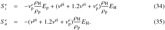 In
Fig. 5 we present the ratios of the rates for electron
impact ionization of hydrogen and helium (singly charged). To enhance the visibility, we
normalized to the charge exchange rate σ(H+ + H) in the following form
In
Fig. 5 we present the ratios of the rates for electron
impact ionization of hydrogen and helium (singly charged). To enhance the visibility, we
normalized to the charge exchange rate σ(H+ + H) in the following form
 (36)where
X ∈ {H, He}. The ratio
r was
estimated from an existing dynamic model with high-speed streams over the poles. The
cross-sections were calculated from the modeled plasma parameters, hence they are not
selfconsistently taken into account. Nevertheless, this demonstrates the relative importance
of electron impact ionization in the heliosphere, which finally has to be modeled
selfconsistently. Figure 5 shows a contribution of
about 20%, as discussed above, especially in the tail region. The significance can be seen
when estimating the Alfvén speed, which is inversely proportional to the square root of the
total density of charged particles. An enhancement of 20% in the charged density (according
to the model by Slavin & Frisch 2008) will
lead to approximately 10% reduction in the Alfvén speed (Scherer & Fichtner 2014). This is important for the recent discussion
about the bow shock (McComas et al. 2012). It can
even be seen in Fig. 5 that the electron impact
ionization is not negligible inside the termination shock.
(36)where
X ∈ {H, He}. The ratio
r was
estimated from an existing dynamic model with high-speed streams over the poles. The
cross-sections were calculated from the modeled plasma parameters, hence they are not
selfconsistently taken into account. Nevertheless, this demonstrates the relative importance
of electron impact ionization in the heliosphere, which finally has to be modeled
selfconsistently. Figure 5 shows a contribution of
about 20%, as discussed above, especially in the tail region. The significance can be seen
when estimating the Alfvén speed, which is inversely proportional to the square root of the
total density of charged particles. An enhancement of 20% in the charged density (according
to the model by Slavin & Frisch 2008) will
lead to approximately 10% reduction in the Alfvén speed (Scherer & Fichtner 2014). This is important for the recent discussion
about the bow shock (McComas et al. 2012). It can
even be seen in Fig. 5 that the electron impact
ionization is not negligible inside the termination shock.
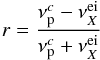
As can be inferred from Fig. 5, the electron impact is significant almost everywhere inside the heliopause and dominates close to the heliopause and in the tail region, at least for the ionization of hydrogen. The structures in the heliotail visible in Fig. 5 are caused by the previous solar cycle activities, which are still propagating down the heliotail (see Scherer & Fahr 2003b,a; Zank & Müller 2003). For our calculations, we estimated the cross-section from the relative velocity and temperature taken from the model, with the assumption of thermal equilibrium. It also shows that our rough approximations above are quite good.
The discussion shows that electron impact effects for hydrogen and helium needs to be taken into account to improve heliospheric models, which otherwise can lead to results that differ in extreme cases by 20% (see Eqs. (30) to (36)).
6. Helium loss in the inner heliosheath
To interpret the IBEX observation for helium and other species (Bzowski et al. 2012) it is important to know how much helium is lost in
the inner heliosheath. To estimate the order of these losses, we used the balance continuity
equation for helium 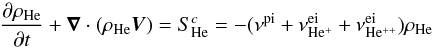 (37)where we took
only the photoionization to singly charged helium from Table C.1 in Appendix C, and the electron impact to both ionization states as losses.
Other losses are small, even the photoionization to the doubly charged state (Rucinski et al. 1996). The plasma is subsonic in the
heliosheath, and the divergence term may be neglected with the usual assumption of
incompressibility for subsonic flows. Nevertheless, because due to the ionization some
particles are lost, this assumption holds no longer true, strickly speaking. If we assume
for the moment that we can neglect the divergence, Eq. (37) has the solution
(37)where we took
only the photoionization to singly charged helium from Table C.1 in Appendix C, and the electron impact to both ionization states as losses.
Other losses are small, even the photoionization to the doubly charged state (Rucinski et al. 1996). The plasma is subsonic in the
heliosheath, and the divergence term may be neglected with the usual assumption of
incompressibility for subsonic flows. Nevertheless, because due to the ionization some
particles are lost, this assumption holds no longer true, strickly speaking. If we assume
for the moment that we can neglect the divergence, Eq. (37) has the solution  (38)with
 . For the following
estimation, we furthermore assumed a lower limit for the photoionization rate at 1 AU
νpi(1 AU) = 8 × 10⁻⁸ s-1 (Rucinski et al. 2003) and that it decreases like r-2, that the
heliosheath has a width of 40 AU, and that the photoionization rate inside the heliosheath
has a constant value νpi(100 AU) = 8 × 10-12 s-1. Since the total temperature in
the heliosheath is 106 K, see Livadiotis et al.
(2011), but also Richardson et al. (2008)
for a lower proton temperature, with the values for the electron impact as discussed above,
we derive τ ≈ 300 years. Particles with speeds of 20, 25, or
30 km s-1 need
≈9.45, 7.56, and 6.29 years to
travel through the inner heliosheath. Inserting these numbers into Eq. (38) leads to a decrease of 2–3% integrated over
that distance. Increasing the distance between the heliopause and termination shock, that is
for higher latitudes or different solar activity, these numbers will increase approximately
linearly.
. For the following
estimation, we furthermore assumed a lower limit for the photoionization rate at 1 AU
νpi(1 AU) = 8 × 10⁻⁸ s-1 (Rucinski et al. 2003) and that it decreases like r-2, that the
heliosheath has a width of 40 AU, and that the photoionization rate inside the heliosheath
has a constant value νpi(100 AU) = 8 × 10-12 s-1. Since the total temperature in
the heliosheath is 106 K, see Livadiotis et al.
(2011), but also Richardson et al. (2008)
for a lower proton temperature, with the values for the electron impact as discussed above,
we derive τ ≈ 300 years. Particles with speeds of 20, 25, or
30 km s-1 need
≈9.45, 7.56, and 6.29 years to
travel through the inner heliosheath. Inserting these numbers into Eq. (38) leads to a decrease of 2–3% integrated over
that distance. Increasing the distance between the heliopause and termination shock, that is
for higher latitudes or different solar activity, these numbers will increase approximately
linearly.
This loss is on the same order as that determined by Cummings et al. (2002), who discussed, in view of anomalous cosmic ray composition, a loss of helium in the heliosheath in the order of 5% in the inner heliosheath. Obviously these losses may be even more pronounced for more extended astrosheaths.
7. Charge exchange with particles of different masses
For the interaction of particles with different mass, the approach by McNutt et al. (1998) can be applied. The calculation of the collision integrals between two species requires knowing the functional form of the charge-exchange cross-section, that is, one has to solve integrals of the form
 where
| g| = |V2 − V1 |
is the modulus of the velocities V1,V2
of the individual particles of species 1 or 2, and the indices { c,m,e } indicate the
integrals for the continuity, momentum and energy equation (see Eq. (A.1)), k ∈ {1, 3}
for {c, e},
respectively. The collision integrals are equivalent to the balance terms Sc,e and Sm, which are
their solution under simplifying assumptions, for an example see below.
where
| g| = |V2 − V1 |
is the modulus of the velocities V1,V2
of the individual particles of species 1 or 2, and the indices { c,m,e } indicate the
integrals for the continuity, momentum and energy equation (see Eq. (A.1)), k ∈ {1, 3}
for {c, e},
respectively. The collision integrals are equivalent to the balance terms Sc,e and Sm, which are
their solution under simplifying assumptions, for an example see below.
In most derivations it is assumed that σcx(g) is nearly constant
(Heerikhuisen et al. 2008; McNutt et al. 1998; Alouani-Bibi et al.
2011). This is in general not the case; even for σcx(H + p) this
holds only below energies of 5 keV. Unfortunately, the integrals
 can only
be solved analytically for a polynomial functional dependence of σcx. The solution
to this dilemma was sketched by McNutt et al. (1998)
by developing σcx into a Taylor series and assuming that
after a given order all higher-order terms vanish. McNutt et
al. (1998) required that only the zeroth order is relevant, and determined the
characteristic speed (
can only
be solved analytically for a polynomial functional dependence of σcx. The solution
to this dilemma was sketched by McNutt et al. (1998)
by developing σcx into a Taylor series and assuming that
after a given order all higher-order terms vanish. McNutt et
al. (1998) required that only the zeroth order is relevant, and determined the
characteristic speed ( ) at which the
cross-sections should be taken. The authors calculated the characteristic speed by inserting
the first order of the Taylor expansion of σcx into the integrals
) at which the
cross-sections should be taken. The authors calculated the characteristic speed by inserting
the first order of the Taylor expansion of σcx into the integrals
 and
requiring that the sum of these integrals vanishes. This allows one to determine a
characteristic speed, which follows mathematically from the mean value theorem for
integrals. Nevertheless, this procedure holds only as long as the cross-sections are weakly
varying. In general, this is not true and as correction the higher-order terms shall be used
(see Appendix B).
and
requiring that the sum of these integrals vanishes. This allows one to determine a
characteristic speed, which follows mathematically from the mean value theorem for
integrals. Nevertheless, this procedure holds only as long as the cross-sections are weakly
varying. In general, this is not true and as correction the higher-order terms shall be used
(see Appendix B).
Moreover, the relative velocities calculated for the collision integrals
 are
mutually distinct and also not identical with the characteristic speeds discussed above, see
also Appendix B. With a notation introduced in
Appendix B, which is slightly different from that of
McNutt et al. (1998), the dimensionless parameter
α reads
are
mutually distinct and also not identical with the characteristic speeds discussed above, see
also Appendix B. With a notation introduced in
Appendix B, which is slightly different from that of
McNutt et al. (1998), the dimensionless parameter
α reads
 (41)with
the individual particle velocities v1,v2
and thermal speeds w1,w2
for the particles of species 1 or 2, respectively. Then one finds that the above-mentioned
different speeds normalized to the thermal speeds are functions of α alone that is
(41)with
the individual particle velocities v1,v2
and thermal speeds w1,w2
for the particles of species 1 or 2, respectively. Then one finds that the above-mentioned
different speeds normalized to the thermal speeds are functions of α alone that is
 , where
j ∈ {c, m, e, P} for the continuity,
momentum, and energy equations and j = P for the thermal pressure,
respectively. The indices i ∈ {cx, rel} are the speeds
needed for the characteristic speeds in the charge exchange cross-section and the
corresponding relative speeds, respectively. All speeds
, where
j ∈ {c, m, e, P} for the continuity,
momentum, and energy equations and j = P for the thermal pressure,
respectively. The indices i ∈ {cx, rel} are the speeds
needed for the characteristic speeds in the charge exchange cross-section and the
corresponding relative speeds, respectively. All speeds
 are called
collision speeds in the following. The explicit formulas are stated in Appendix B.
are called
collision speeds in the following. The explicit formulas are stated in Appendix B.
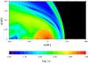 |
Fig. 6 α parameter throughout the heliosphere. α is the ratio of the modulus of the relative bulk velocity to the thermal speed of the two species, see Eq. (41). |
In Fig. 6 the parameter α is presented throughout the
heliosphere. It can be seen that it ranges from values near zero close to the heliopause, in
the tail region, and in the outer heliosheath, where the relative velocities are low, but
the thermal ones high, to values in the range of 30 inside the termination shock, where the
relative velocity is high and the thermal speed low. In the left panel of Fig. 7 the dependence of the
 from
α is shown
and in the right panel of Fig. 7 the relative “error”
from
α is shown
and in the right panel of Fig. 7 the relative “error”
 is
presented.
is
presented.
The collision speeds for the continuity equations nicely follow the approximation
 for
α > 1, while the speeds
for
α > 1, while the speeds
 and
and
 for the
momentum and energy equation, respectively, differ strongly for all values of
α, as well as
those for the continuity equations for small α, as can be nicely seen in the right panel of Fig.
7.
for the
momentum and energy equation, respectively, differ strongly for all values of
α, as well as
those for the continuity equations for small α, as can be nicely seen in the right panel of Fig.
7.
 |
Fig. 7 Characteristic collision speeds normalized to the thermal speed as a function of the
parameter α (left panel) and the relative
“error” |
With these speeds, the charge exchange terms read
![\begin{eqnarray} && S_{i}^{c} = \pm \frac{\rho_{1}\rho_{2}}{m_{i}} \sigma^{\rm cx}(u_{c}^{\rm cx}) u_{c}^{\rm rel}\\ &&S_{i}^{m} = \pm \frac{\rho_{1}\rho_{2}}{m_{1}+m_{2}}\sigma^{\rm cx}(u_{m}^{\rm cx}) u_{m}^{\rm rel}\Delta \vec{v}\\[-2mm] &&S_{i}^{e}= \pm \frac{\rho_{1}\rho_{2}}{m_{1}+m_{2}} \Bigg(\frac{2k_{\rm B}(T_{2}-T_{1})}{m_{1}+m_{2}}\sigma^{\rm cx}(u_{e}^{\rm cx})u_{e}^{\rm rel}\\[-2mm] \nonumber &&\qquad +~ \sigma^{\rm cx}(u_{m}^{\rm cx})u_{m}^{\rm rel}(v_{1}^{2}+v_{2}^{2}) + \frac{1}{2}\frac{w_{2}^{2}-w_{1}^{2}}{w_{1}^{2}+m_{2}^{2}}\sigma^{\rm cx}(u_{m}^{\rm cx})u_{m}^{\rm rel}(\Delta v)^{2}\Bigg). \end{eqnarray}](/articles/aa/full_html/2014/03/aa21151-13/aa21151-13-eq189.png) In
these formulas i ∈ {1, 2} stands for the
respective particle species, and the ± sign has to be chosen in such a way that a loss in one species (for
example, ions) is a gain in another one (for example, fast neutrals).
In
these formulas i ∈ {1, 2} stands for the
respective particle species, and the ± sign has to be chosen in such a way that a loss in one species (for
example, ions) is a gain in another one (for example, fast neutrals).
Even when the neutrals are treated kinetically (Izmodenov et al. 2005; Heerikhuisen et al. 2008), the moments of the collision integrals must be calculated, because the ions are handled with an MHD approach, in which implicitly the solution of those for Maxwellian-distributed particles are modeled. Thus, these calculations have to be repeated with a different velocity distribution, for instance, a κ-distribution (Heerikhuisen et al. 2008), to obtain the required collision speeds.
Moreover, as discussed briefly in Appendix B, this
discussion is only valid when the cross-sections are mainly independent of the collision
speeds  . This is in
general not true; even for the reaction H + p this holds only for energies (speeds) below 5 keV (≈1000 km s-1), and thus the assumption of a
nearly constant cross-section may not be valid for high-speed streams of the solar wind, nor
even for astrospheres of hot stars, where the speed is on the order on a few
1000 km s-1. Thus
higher-order approximations of the Taylor expansions are required. Because this leads to
clumsy expressions, which also need a lot of computational effort, it may be better for
practical purposes to solve the collision integrals numerically as in Fichtner et al. (1996).
. This is in
general not true; even for the reaction H + p this holds only for energies (speeds) below 5 keV (≈1000 km s-1), and thus the assumption of a
nearly constant cross-section may not be valid for high-speed streams of the solar wind, nor
even for astrospheres of hot stars, where the speed is on the order on a few
1000 km s-1. Thus
higher-order approximations of the Taylor expansions are required. Because this leads to
clumsy expressions, which also need a lot of computational effort, it may be better for
practical purposes to solve the collision integrals numerically as in Fichtner et al. (1996).
8. Astrospheres revisited
Most of the aspects discussed above hold in general for astrospheres. Nevertheless, because the stellar winds and the interstellar medium can be very different from that of the heliosphere, care must be taken which of the collision channels displayed in Tables C.1 and C.2 needs to be taken into account. For example, a stellar wind of 2000 km s-1 has kinetic energies of about 20 keV and most of the interactions become important. Such wind speeds were derived by Vidotto et al. (2011) and are common in winds around hot stars (Arthur 2012; Decin et al. 2012). For such astrospheres, there may be strong bow shocks, because the interstellar wind is comparatively strong. We may then encounter the situation where the low first ionization potential (FIP) elements cannot reach the inner astrosheath, but the high-FIP elements do. This is an interesting aspect when discussing the acceleration of energetic particles. Such a filtering of low-FIP elements occurs in the heliosphere concerning carbon, which becomes easily ionized already in the interstellar medium and thus cannot penetrate into the heliosphere (Cummings et al. 2002).
In astrospheres additional effects can play a role, such as elastic collisions into an excited atomic state and subsequent photon emission, thus energy loss. Recombination can take place, as well as Bremsstrahlung or synchrotron radiation, when a strong enough magnetic field is present, which can lead to additional cooling of the stellar wind plasma.
Astrospheres show a variety of shapes, and all can be described by the set of (hybrid) (M)HD equations discussed in Appendix A. If the surrounding interstellar medium is partially ionized, it must be carefully determined which of the charge exchange reactions play a role. Especially, the charge exchange between particles with different masses needs to be carefully implemented, because in the collision integrals mi/(mi + mj) (where mi,mj denote the corresponding mass of species i,j) appears as a factor.
9. Conclusions
We have demonstrated that electron impact ionizations are important processes inside the heliopause and particularly in the heliosheath, while other charge exchange processes, except for that of H+ + H → H+ + H, have been neglected because of their small cross-sections for solar wind speeds. They become important when modeling astrospheres, where the stellar wind speeds can be higher by a factor 5 or more (up to 3000 km s-1, see Arthur 2012). In that case it is evident from Fig. 2 that a thorough discussion of the charge exchange between hydrogen and helium atoms, both neutral and ionized, is needed. The newly generated PUIs heat the stellar wind even inside the termination shock, so that the threshold for electron impact ionization is exceeded, and here electron impact plays a role, which then can additionally diminish the neutral helium density by 3%.
Care must also be taken because the cross-sections are taken from a fit curve that may deviate by up to 10% from the data, see also the discussion by Bzowski et al. (2013). Moreover, for the continuity, momentum, and energy equations the different collision speeds need to be taken into account in the modeling efforts. Additionally, depending on the representation of the cross-sections, the assumption that they are nearly constant, as in McNutt et al. (1998), and Heerikhuisen et al. (2008) over a wide range, does not hold anymore. Therefore, either higher-order corrections in the Taylor expansion of the cross-sections need to be taken into account, or a numerical estimation of the collision integrals is needed in modeling the heliosphere or astrospheres.
Especially for astrospheres, which can have relative speeds of a few thousand kilometers per second, the nonresonant charge exchange processes for helium become increasingly important. For the huge astrospheres of O-stars of tens of parsecs (Arthur 2012) the ionization of other species should be carefully considered, because they can play a role in heating the supersonic stellar wind.
Moreover, during high-speed solar wind streams or coronal mass ejections traveling into the outer regions of the heliosphere the dynamics of the solar wind and propagating shock fronts of CMEs will be influenced by charge exchange processes, including electron impact, and by different helium ionizing processes.
For (M)HD simulations, one can use the governing equations, that is, one set of Euler equations for the combined ions and one for the sum of neutrals. The densities of all included species can be handled with a test particle approach, that is, only solving the corresponding continuity equation to derive the correct density distribution in the heliosphere. A better strategy is to solve in addition the energy equation for each species to compute their contribution to the total pressure selfconsistently. In the governing energy equation a sophisticated heat transport can also be included. In a forthcoming work we will include these processes in our model, specifically add a new species, helium, as well as the heat flow caused by the electrons, and study the relevance of all these effects.
Finally, there are clear indications that the electrons downstream of the termination shock can easily attain much higher temperatures compared than those of the protons (Chalov & Fahr 2013).
We also point out that the He+ abundance modeled by Slavin & Frisch (2008) reduces the Alfvén speed by about 10%, which again shows the importance of including helium in models.
We have shown here that all charge exchange processes need to be reanalyzed carefully to minimize the errors in large-scale models and to improve the fits to the newly available IBEX and Voyager data.
Online material
Appendix A: Set of MHD equations
A general set of the Eulerian continuity-, momentum-, and energy equations is the
following (see e.g. Boyd & Sanderson
2003): ![\appendix \setcounter{section}{1} \begin{eqnarray} \label{ap:1} \del \begin{bmatrix} \rho_{j} \\ \rho_{j} \vec{v}_{j} \\ E_{j}\\\vec{B} \end{bmatrix} +\div \begin{bmatrix} \rho_{j} \vec{v}_{j} \\ \rho_{j} \vec{v}_{j}\vec{v}_{j} + P_{j} \hat{I} - \dfrac{\vec{B}\vec{B}}{4\pi}\\[0.25cm] (E_{j} + P_{j})\vec{v}_{j} -\dfrac{\vec{B}(\vec{B}\cdot\vec{v_{j}})}{4\pi} \\ \vec{v}_{j}\vec{B}-\vec{B}\vec{v}_{j} \end{bmatrix} =\nonumber\\ \begin{bmatrix} 0 \\ \rho_{j} \vec{F} + \div \hat{\sigma}\\ \rho_{j} \vec{v}_{j}\cdot\vec{F} + \div (\vec{v}_{j}\cdot\hat{\sigma}) - \div \vec{Q}\\0\end{bmatrix} + \begin{bmatrix} S_{j}^{c} \\ \vec{S}_{j}^{m}\\S_{j}^{e}\\A_{j}\end{bmatrix} \end{eqnarray}](/articles/aa/full_html/2014/03/aa21151-13/aa21151-13-eq197.png) (A.1)
(A.1)
-
vj= fluid velocity
-
ρj= fluid density
-
Ej= internal energy of fluid
-
Pj= pressure of fluid
-
Î= unit tensor
-
 =
viscosity/stress tensor
=
viscosity/stress tensor -
F= external force per unit mass and volume
-
Q= heat flow
-
 =
sources and sinks
=
sources and sinks -
Aj= ambipolar diffusion between ions and neutrals
where the index j ∈ { H,H+,He,He+,He+ +,i,n }. As discussed above for the index j of the ionized fluid, the density is the sum of all densities of ionized species, the total pressure Pj = ∑ kPk, the total energy Ej = ∑ kEk, with k ∈ {H+, He+, He+ + }.
The force densities, stress tensor and the heat transport on the right-hand side of Eq.
(A.1) are usually neglected in
modeling the large-scale structure of the heliosphere, that is,
 .
While external forces, such as solar gravitation, can be neglected, the stress tensor
will play an important role in studying the details of the termination shock or
heliopause structure, but to our knowledge this was not discussed so far. Especially the
heat transport by electrons can be expected to be significant, because of the high
thermal speed of these particles, and will be analyzed in future work. If the right-hand
side of Eq. (A.1) vanishes, the set of
equations is called ideal MHD.
.
While external forces, such as solar gravitation, can be neglected, the stress tensor
will play an important role in studying the details of the termination shock or
heliopause structure, but to our knowledge this was not discussed so far. Especially the
heat transport by electrons can be expected to be significant, because of the high
thermal speed of these particles, and will be analyzed in future work. If the right-hand
side of Eq. (A.1) vanishes, the set of
equations is called ideal MHD.
From Eq. (27) it is evident that the interstellar helium contributes about 40% to the total mass density, thus the total mass density ρn in the above neutral continuity equation is ρn = ρH + ρHe ≈ 1.4ρH. This results in an increased ram pressure and momentum flow ρnvn. Together with the total pressure Pn = PH + PHe = κ(nHTH + nHeTHe) and the previously made assumption TH = THe and nHe = 0.1nH yields Pn = 1.1PH. These estimates show, that helium contributions are not negligible. A similar consideration holds for the governing equations of the charged particles.
If the helium inflow velocity differs in direction from that of hydrogen (Lallement et al. 2005), helium has to be treated as a separate fluid and an additional complete set of the Euler-equations must be solved. If one can assume that the flow velocities of the neutrals and charged fluids are the same for all neutral and ionized species, it is sufficient to solve the two governing equations and treat the other species as tracer particles to calculate their densities and thermal pressures.
Handling the neutrals with a kinetic set of equations (Izmodenov 2007; Heerikhuisen et al.
2008) requires a similar approach for the collision integrals (see Eqs. (39) and (40)) to obtain the balance terms
 for the
(M)HD equations of charged particles, when including heavier ions.
for the
(M)HD equations of charged particles, when including heavier ions.
Appendix B: “Collision” speeds
For the interaction of particles with different masses (nonresonant charge exchange processes), the approach by McNutt et al. (1998) can be applied. Nevertheless, the relative velocities for the momentum exchange differ from those for the energy exchange, in contrast to what was discussed in McNutt et al. (1998)
 As
described in Eqs. (57) to (60) in McNutt et al.
(1998), the relative speeds for the cross-sections for charge exchange differ
for all three Euler equations, as well as the speeds needed for the charge exchange
cross-section. The speeds are denoted as above , where
j ∈ {c, m, e, P} for the
continuity, momentum, and energy equations and j = P
for the thermal pressure, respectively. The governing energy equation contains the ram
pressure and the thermal pressure, which are both influenced. The balance equations only
contain the thermal pressure, because changes in the ram pressure or bulk speed are
calculated in the governing equations with the assumption that all species flow with the
same speed. The indices i ∈ {cx, rel} are the speeds
needed for the charge exchange cross-section and corresponding relative speeds. With the
definitions from McNutt et al. (1998) we have to
solve the following type of integrals:
As
described in Eqs. (57) to (60) in McNutt et al.
(1998), the relative speeds for the cross-sections for charge exchange differ
for all three Euler equations, as well as the speeds needed for the charge exchange
cross-section. The speeds are denoted as above , where
j ∈ {c, m, e, P} for the
continuity, momentum, and energy equations and j = P
for the thermal pressure, respectively. The governing energy equation contains the ram
pressure and the thermal pressure, which are both influenced. The balance equations only
contain the thermal pressure, because changes in the ram pressure or bulk speed are
calculated in the governing equations with the assumption that all species flow with the
same speed. The indices i ∈ {cx, rel} are the speeds
needed for the charge exchange cross-section and corresponding relative speeds. With the
definitions from McNutt et al. (1998) we have to
solve the following type of integrals:  (B.1)The
following recursion holds:
(B.1)The
following recursion holds:  (B.2)Thus
we need only to know the four integrals (Gradstein
& Ryshik 1981), Nr. 3.562.3-3562.6:
(B.2)Thus
we need only to know the four integrals (Gradstein
& Ryshik 1981), Nr. 3.562.3-3562.6:
 These
integrals need to be multiplied by the factors given in McNutt et al. (1998).
These
integrals need to be multiplied by the factors given in McNutt et al. (1998).
With these integrals it is easy to calculate the required speeds (for details see McNutt et al. 1998):
![\appendix \setcounter{section}{2} \begin{eqnarray} \label{eq:a4} &&\nonumber\\[-6mm] &&u_{\rm rel}^{m,I_{\rm coll}} = \frac{1}{\sqrt{\kappa}} \left(-\frac{1}{4\alpha^{3}}+\frac{1}{\alpha}+\alpha \right)\erf(\alpha) + \left(2 + \frac{1}{\alpha^{2}}\right)\dfrac{{\rm e}^{-a^{2}}}{\sqrt{\pi}}\nonumber\\ &&\qquad\; \; \approx\frac{2}{\sqrt{\kappa}}\sqrt{\frac{64}{9\pi}+\alpha^{2}}\\\label{eq:a5} &&u_{\rm rel}^{m,\sigma}= \frac{1}{\kappa}\dfrac{\frac{5}{2}+\alpha^{2}}{u_{\rm rel}^{m,I_{\rm coll}}}\approx \frac{1}{2\sqrt{\kappa}}\sqrt{\frac{225\pi}{256}+\alpha^{2}}\\\label{eq:a6} &&u_{\rm rel}^{e,I_{\rm coll}}= \frac{1}{\sqrt{\kappa}} \left(\frac{3}{4\alpha} + 3\alpha+\alpha^{3} \right) \erf{\alpha} + \left(\frac{5}{2}+\alpha^{2} \right)\dfrac{{\rm e}^{-\alpha^{2}}}{\sqrt{\pi}} \\\label{eq:a7} &&u_{\rm rel}^{e,\sigma} = \frac{1}{\kappa} \dfrac{\frac{15}{4}+5\alpha^{2}+\alpha^{4}}{2 u_{\rm rel}^{c,I_{\rm coll}}+\alpha^{2}u_{\rm rel}^{m,I_{\rm coll}}}\cdot \end{eqnarray}](/articles/aa/full_html/2014/03/aa21151-13/aa21151-13-eq229.png) The
approximations in Eqs. (B.3) to (B.8) fit nicely, except for small errors
(see Fig. B.1). Note that the fit in Eq. (B.6) differs by a factor 0.5 from that of
McNutt et al. (1998).
The
approximations in Eqs. (B.3) to (B.8) fit nicely, except for small errors
(see Fig. B.1). Note that the fit in Eq. (B.6) differs by a factor 0.5 from that of
McNutt et al. (1998).
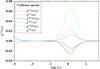 |
Fig. B.1 Relative errors |

With the help of the integrals  it is
easy to calculate the higher-order correction terms. However, this is not necessary for
the p + H reaction, because
the second-order derivatives of the cross-sections, as shown in Fig. B.1, are orders of magnitudes lower than the
cross-section. Shown in Fig. B.2 are the functional
dependencies given by Fite et al. (1962) and by
Lindsay & Stebbings (2005), that is
it is
easy to calculate the higher-order correction terms. However, this is not necessary for
the p + H reaction, because
the second-order derivatives of the cross-sections, as shown in Fig. B.1, are orders of magnitudes lower than the
cross-section. Shown in Fig. B.2 are the functional
dependencies given by Fite et al. (1962) and by
Lindsay & Stebbings (2005), that is
![\appendix \setcounter{section}{2} \begin{eqnarray} && \sigma_{\rm F} = [2.6\times 10^{-7}-9.2\times 10^{-9}\ln(v_{\rm rel})]^{2}\\\nonumber && \sigma_{\rm LS}= [22.8-1.09\ln(v_{\rm rel})]^{2}\times \left(1-\exp\left\{-\frac{1.3\times 10^{17}}{v_{\rm rel}^{2}}\right\}\right)^{2} \end{eqnarray}](/articles/aa/full_html/2014/03/aa21151-13/aa21151-13-eq235.png) (B.9)where
vrel is given in cm/s and the
σ in
cm2.
(B.9)where
vrel is given in cm/s and the
σ in
cm2.
With the help of the computer algebra system wxMaxima3 it is easy to calculate the second derivatives of these commonly used
cross-sections for the p + H
reaction and the integrals for the second-order terms of the Taylor-expansion for
σcx. For the terms needed in the
continuity equation, we have to compare  with the
second-order terms
with the
second-order terms  ,
where we neglected common factors for simplicity. In our notation
,
where we neglected common factors for simplicity. In our notation
 . With some
algebra, we find that
. With some
algebra, we find that  and thus finally
 (B.10)The
function h(v) defined above is small for
all v, so
that we can assume that the higher-order terms in the Taylor expansion of
σcx vanish. In Fig. B.2 the function is shown for the two cross-sections.
(B.10)The
function h(v) defined above is small for
all v, so
that we can assume that the higher-order terms in the Taylor expansion of
σcx vanish. In Fig. B.2 the function is shown for the two cross-sections.
 |
Fig. B.2 Ratio h(v) (Eq. (B.10)) of the second-order integrated Taylor-expansion to the zeroth order for the two H-p charge exchange cross-sections discussed by Fite et al. (1962) and Lindsay & Stebbings (2005). The bump between the two downward spikes in the Lindsay-Stebbings curve is negative, but to represent it in a logarithmic scale, its absolute value was taken. See text for restrictions of the fit functions. |
It can be seen in Fig. B.2 that for the Fite et al. (1962) cross-section the second-order terms are nearly a factor 10 lower than the zeroth-order term for all speeds. For the Lindsay & Stebbings (2005) cross-sections this holds only for speeds lower than 4 × 107 cm/s = 400 km s-1. Around these speeds, that is, a commonly used solar wind speed, the second-order corrections are on the same order than the zeroth-order term.
Gains and losses from the original populations.
In the latter case, that is, if the higher-order terms cannot be neglected, in the analytic representation this will lead to clumsy formulas, which also need some computational time. Thus, it might be better to solve the collision integrals numerically.
Note, that for the hydrogen-proton reactions the fit function discussed in Fite et al. (1962) has an upper boundary of 10 keV, which corresponds to a relative speed of ≈1400 km s-1. The range in which the data were fitted by Lindsay & Stebbings (2005) has an upper boundary of 300 keV, which corresponds to a speed lower than ≈7500 km s-1. The data presented in Fig. 2 were taken from the Redbooks4 and reach to 63 keV, corresponding to ≈3400 km s-1. Some of the helium reactions have their maximum cross-section at higher energies, as can be seen in Table C.1, and their upper limits in energy/amu are higher than shown in Fig. 2.
All the fits given for the data from the Redbooks or the Aladdin database are mainly based upon a fit with Chebyshev polynomials. These polynomial fits are only good in the range given by the corresponding upper and lower (energy) boundaries and cannot be extended beyond these. Because usually it cannot be guaranteed in a large-scale model that the relative speeds are always in that range, a better fit function is needed, which can be extended beyond the boundaries, keeping in mind not to violate quantum mechanical requirements.
We here only discussed the simplest case, that is, the collision terms for the continuity equation. Of course this analysis must be performed not only for the remaining set of MHD equations, but has, especially, to be verified for all interactions.
Appendix C: Interaction terms
Gains from the new populations.
In the following we provide an overview of possible ionization reactions. In Table C.1, the first column gives the interaction term in the continuity equation, indicating the particle species: Xn with X∈ {H,He}, while n ∈ { 0,1,2 } gives the ionization state (usually the index 0 is omitted). Newly created ions are named as PUIXn and energetic atoms by ENAX. The reaction rates have the indices {cx, ei, pi} for charge exchange, electron impact, and photoionization, respectively. The rates are also denoted by ν(i,j), where i describes different reactants, while j stands for different products of the same reaction i. The tuple (i,j) is given in the fourth column, where a minus sign stands for losses and a plus sign for gains. To derive the total gains and losses one has to sum over all { i,j }. In the fifth and sixth column the maximal cross-section and its corresponding relative speed is given, respectively. In the third column the first reactant is a particle from the solar wind, while the second reactant is from the interstellar medium. This distinction is necessary to ensure correct sorting.
Note that in the charge exchange rate νcx = ρXσcxvrel the density of the first reactant is included and is indicated in the table by νcx,X.
Table C.1 contains the losses, Table C.2 the gains. In Table C.1 the approximate highest values for the cross-section are listed. They may vary by a factor of three and only indicate the correct order of magnitude. If a range is given for the corresponding relative velocity, the cross-section is a flat curve in that range.
All reactions that have a charged particle as the second reactant cannot flow in from the interstellar medium. Because the heliopause is a contact discontinuity that separates the solar wind and interstellar medium plasma, there is no flow of charged particles across the heliopause. Thus in Tables C.1 and C.2 the reactions labeled (3,1), (4,1), (5,1), (6,1), (8,1), (10,1), and (12,1) can be neglected.
The reactions labeled with an asterisk are sorted in pickup channels, even though they do not create new PUIs. For example, the reaction He+++H→He++H+ produces a new pickup hydrogen, but the change from doubly to singly charged helium does not change its character, that is He+ has the same bulk speed as He2+. Only the charge is changed, thus the new He+ does not
affect the dynamics (the H+ does). Nevertheless, these processes can have an effect on magnetic field turbulence (e.g. Shalchi et al. 2012). This aspect is interesting in the description of the diffusion tensor to model cosmic rays (Effenberger et al. 2012). The role of these types of processes for the turbulence will also be considered in future work.
From these tables the interaction terms for the governing equations can be determined.
For the neutral equation it is just the sum of all
 interaction
terms. More care must be taken for the ion governing equation, because the pickup terms
can cancel some of the ion terms, for example, the reaction H+ + H → H + H+ looses an original fast solar
wind proton, but gains a slow interstellar hydrogen atom, which does not change the
total ion mass.
interaction
terms. More care must be taken for the ion governing equation, because the pickup terms
can cancel some of the ion terms, for example, the reaction H+ + H → H + H+ looses an original fast solar
wind proton, but gains a slow interstellar hydrogen atom, which does not change the
total ion mass.
To describe the interaction terms for the momentum and energy equation, similar tables can now easily be constructed and the governing equations determined.
Acknowledgments
K.S. and H.F. are grateful to the Deutsche Forschungsgemeinschaft, DFG for funding the projects FI706/15-1 and SCHE334/10-1. M.B. was supported by the Polish Ministry for Science and Higher Education grant N-N203-513-038, managed by the National Science Centre. S.E.S.F. thanks the South African National Research Foundation for financial support.
References
- Aleksashov, D. B., Izmodenov, V. V., & Grzedzielski, S. 2004, Adv. Space Res., 34, 109 [NASA ADS] [CrossRef] [Google Scholar]
- Alouani-Bibi, F., Opher, M., Alexashov, D., Izmodenov, V., & Toth, G. 2011, ApJ, 734, 45 [NASA ADS] [CrossRef] [Google Scholar]
- Arnal, E. M. 2001, AJ, 121, 413 [NASA ADS] [CrossRef] [Google Scholar]
- Arnaud, M., & Rothenflug, R. 1985, A&AS, 60, 425 [NASA ADS] [Google Scholar]
- Arthur, S. J. 2012, MNRAS, 421, 1283 [NASA ADS] [CrossRef] [Google Scholar]
- Asplund, M., Grevesse, N., Sauval, A. J., & Scott, P. 2009, ARA&A, 47, 481 [NASA ADS] [CrossRef] [Google Scholar]
- Badnell, N. R. 2006, A&A, 447, 389 [NASA ADS] [CrossRef] [EDP Sciences] [Google Scholar]
- Baranov, V. B., & Malama, Y. G. 1993, J. Geophys. Res., 98, 15157 [NASA ADS] [CrossRef] [Google Scholar]
- Baranov, V. B., Krasnobaev, K. V., & Kulikovskii, A. G. 1971, Soviet Physics Doklady, 15, 791 [Google Scholar]
- Baranov, V. B., Izmodenov, V. V., & Malama, Y. G. 1998, J. Geophys. Res., 103, 9575 [NASA ADS] [CrossRef] [Google Scholar]
- Ben-Jaffel, L., & Ratkiewicz, R. 2012, A&A, 546, A78 [NASA ADS] [CrossRef] [EDP Sciences] [Google Scholar]
- Ben-Jaffel, J., Strumik, M., Ratkiewicz, R., & Grygorczuk, J. 2013, ApJ, 779, 130 [NASA ADS] [CrossRef] [Google Scholar]
- Blasi, P., Morlino, G., Bandiera, R., Amato, E., & Caprioli, D. 2012, ApJ, 755, 121 [NASA ADS] [CrossRef] [Google Scholar]
- Borovikov, S. N., Pogorelov, N. V., Burlaga, L. F., & Richardson, J. D. 2011, ApJ, 728, L21 [NASA ADS] [CrossRef] [Google Scholar]
- Boyd, T. J. M., & Sanderson, J. J. 2003, The Physics of Plasmas (Cambridge University Press) [Google Scholar]
- Bzowski, M., Möbius, E., Tarnopolski, S., Izmodenov, V., & Gloeckler, G. 2008, A&A, 491, 7 [NASA ADS] [CrossRef] [EDP Sciences] [Google Scholar]
- Bzowski, M., Kubiak, M. A., Möbius, E., et al. 2012, ApJS, 198, 12 [NASA ADS] [CrossRef] [Google Scholar]
- Bzowski, M., Sokół, J., Tokumaru, M., et al. 2013, in Cross-Calibration of Past and Present Far UV Spectra of Solar System Objects and the Heliosphere, eds. M. S. R.M. Bonnet, & E. Quémrais, ISSI Scientific Report Series 13 (New York: Springer Science +Business Media), 67 [Google Scholar]
- Cabrera-Trujillo, R. 2010, Plasma Sources Sci. Technol., 19, 034006 [NASA ADS] [CrossRef] [Google Scholar]
- Chalov, S. V., & Fahr, H. J. 2013, MNRAS, 433, L40 [NASA ADS] [Google Scholar]
- Cichowolski, S., Arnal, E. M., Cappa, C. E., Pineault, S., & St-Louis, N. 2003, MNRAS, 343, 47 [NASA ADS] [CrossRef] [Google Scholar]
- Cummings, A. C., Stone, E. C., & Steenberg, C. D. 2002, ApJ, 578, 194 [NASA ADS] [CrossRef] [Google Scholar]
- Dayeh, M. A., McComas, D. J., Allegrini, F., et al. 2012, ApJ, 749, 50 [NASA ADS] [CrossRef] [Google Scholar]
- de Avillez, M. A., & Breitschwerdt, D. 2012, A&A, 539, L1 [NASA ADS] [CrossRef] [EDP Sciences] [Google Scholar]
- Decin, L., Cox, N. L. J., Royer, P., et al. 2012, A&A, 548, A113 [NASA ADS] [CrossRef] [EDP Sciences] [Google Scholar]
- Effenberger, F., Fichtner, H., Scherer, K., et al. 2012, ApJ, 750, 108 [NASA ADS] [CrossRef] [Google Scholar]
- Fahr, H. J. 1968, Ap&SS, 2, 474 [NASA ADS] [CrossRef] [Google Scholar]
- Fahr, H. J. 1979, A&A, 77, 101 [NASA ADS] [Google Scholar]
- Fahr, H.-J. 2004, Adv. Space Sci., 34, 3 [Google Scholar]
- Fahr, H. J. 2007, Ann. Geophys., 25, 2649 [NASA ADS] [CrossRef] [Google Scholar]
- Fahr, H.-J., & Fichtner, H. 1995, Sol. Phys., 158, 353 [NASA ADS] [Google Scholar]
- Fahr, H. J., & Ruciński, D. 1999, A&A, 350, 1071 [NASA ADS] [Google Scholar]
- Fahr, H. J., & Ruciński, D. 2001, Space Sci. Rev., 97, 407 [NASA ADS] [CrossRef] [Google Scholar]
- Fahr, H., & Scherer, K. 2004a, Ann. Geophys., 22, 2229 [NASA ADS] [CrossRef] [Google Scholar]
- Fahr, H. J., & Scherer, K. 2004b, A&A, 421, L9 [NASA ADS] [CrossRef] [EDP Sciences] [Google Scholar]
- Fahr, H. J., Kausch, T., & Scherer, H. 2000, A&A, 357, 268 [NASA ADS] [Google Scholar]
- Fahr, H.-J., Fichtner, H., & Scherer, K. 2007, Rev. Geophys., 45, 4003 [NASA ADS] [CrossRef] [Google Scholar]
- Fahr, H.-J., Siewert, M., & Chashei, I. 2012, Ap&SS, 341, 265 [Google Scholar]
- Fichtner, H., Sreenivasn, S. R., & Vormbrock, N. 1996, J. Plasma Phys., 55, 95 [NASA ADS] [CrossRef] [Google Scholar]
- Fite, W. L., Smith, A. C. H., & Stebbings, R. F. 1962, Proc. Roy. Soc. A, 286, 527 [Google Scholar]
- Funsten, H. O., Allegrini, F., Crew, G. B., et al. 2009, Science, 326, 964 [Google Scholar]
- Gerbig, D., & Schlickeiser, R. 2007, ApJ, 664, 750 [NASA ADS] [CrossRef] [Google Scholar]
- Gershman, D. J., Zurbuchen, T. H., Fisk, L. A., et al. 2012, J. Geophys. Res., 117, [Google Scholar]
- Gloeckler, G., & Geiss, J. 1998, Space Sci. Rev., 86, 127 [NASA ADS] [CrossRef] [Google Scholar]
- Gradstein, I. S., & Ryshik, I. M. 1981, Summen, Produkt- Und Integraltafeln (Harri Deutsch) [Google Scholar]
- Gruntman, M. A. 1982, Sov. Astron. Lett., 8, 24 [NASA ADS] [Google Scholar]
- Grzedzielski, S., Bzowski, M., Czechowski, A., et al. 2010, ApJ, 715, L84 [NASA ADS] [CrossRef] [Google Scholar]
- Heerikhuisen, J., Florinski, V., & Zank, G. P. 2006, J. Geophys. Res., 111, 6110 [Google Scholar]
- Heerikhuisen, J., Pogorelov, N. V., Florinski, V., Zank, G. P., & le Roux, J. A. 2008, ApJ, 682, 679 [NASA ADS] [CrossRef] [Google Scholar]
- Isenberg, P. A. 1995, Rev. Geophys., 33, 623 [NASA ADS] [CrossRef] [Google Scholar]
- Izmodenov, V., Malama, Y. G., Gloeckler, G., & Geiss, J. 2003, ApJ, 594, L59 [NASA ADS] [CrossRef] [Google Scholar]
- Izmodenov, V., Malama, Y., & Ruderman, M. S. 2005, A&A, 429, 1069 [NASA ADS] [CrossRef] [EDP Sciences] [Google Scholar]
- Izmodenov, V. V. 2007, Space Sci. Rev., 130, 377 [NASA ADS] [CrossRef] [Google Scholar]
- Izmodenov, V. V., & Baranov, V. B. 2006, ISSI Scientific Rep. Ser., 5, 67 [Google Scholar]
- Izmodenov, V. V., Malama, Y. G., & Ruderman, M. S. 2008, Adv. Space Res., 41, 318 [NASA ADS] [CrossRef] [Google Scholar]
- Kingdon, J. B., & Ferland, G. J. 1996, ApJS, 106, 205 [NASA ADS] [CrossRef] [Google Scholar]
- Koutroumpa, D., Lallement, R., Kharchenko, V., & Dalgarno, A. 2009, Space Sci. Rev., 143, 217 [NASA ADS] [CrossRef] [Google Scholar]
- Lallement, R., Quémerais, E., Bertaux, J. L., et al. 2005, Science, 307, 1447 [NASA ADS] [CrossRef] [Google Scholar]
- Lallement, R., Quémerais, E., Koutroumpa, D., et al. 2010, in Twelfth International Solar Wind Conf., 1216, 555 [Google Scholar]
- Lamers, H. J. G. L. M., & Cassinelli, J. P. 1999, Introduction to Stellar Winds (Cambridge: Cambridge University Press) [Google Scholar]
- Lenchek, A. M. 1964, Annales d’Astrophysique, 27, 219 [NASA ADS] [Google Scholar]
- Lie-Svendsen, Ø., Hansteen, V. H., & Leer, E. 2003, ApJ, 596, 621 [NASA ADS] [CrossRef] [Google Scholar]
- Lindsay, B. G., & Stebbings, R. F. 2005, J. Geophys. Res., 110, 12213 [NASA ADS] [CrossRef] [Google Scholar]
- Livadiotis, G., McComas, D. J., Dayeh, M. A., Funsten, H. O., & Schwadron, N. A. 2011, ApJ, 734, 1 [NASA ADS] [CrossRef] [Google Scholar]
- Lotz, W. 1967, ApJS, 14, 207 [NASA ADS] [CrossRef] [Google Scholar]
- Lotz, W. 1970, Z. Phys., 232, 101 [Google Scholar]
- Maher, L. J., & Tinsley, B. A. 1977, J. Geophys. Res., 82, 689 [NASA ADS] [CrossRef] [Google Scholar]
- Maksimovic, M., Pierrard, V., & Riley, P. 1997, Geophys. Res. Lett., 24, 1151 [NASA ADS] [CrossRef] [Google Scholar]
- Malama, Y. G., Izmodenov, V. V., & Chalov, S. V. 2006, A&A, 445, 693 [NASA ADS] [CrossRef] [EDP Sciences] [Google Scholar]
- Marsch, E., Rosenbauer, H., Schwenn, R., Muehlhaeuser, K.-H., & Neubauer, F. M. 1982, J. Geophys. Res., 87, 35 [Google Scholar]
- Mattioli, M., Mazzitelli, G., Finkenthal, M., et al. 2007, J. Phys. B At. Mol. Phys., 40, 3569 [NASA ADS] [CrossRef] [Google Scholar]
- Mazzotta, P., Mazzitelli, G., Colafrancesco, S., & Vittorio, N. 1998, A&AS, 133, 403 [Google Scholar]
- McComas, D. J., Allegrini, F., Bochsler, P., et al. 2009, Space Sci. Rev., 146, 11 [NASA ADS] [CrossRef] [Google Scholar]
- McComas, D. J., Dayeh, M. A., Allegrini, F., et al. 2012, ApJS, 203, 1 [NASA ADS] [CrossRef] [Google Scholar]
- McNutt, Jr., R. L., Lyon, J., & Goodrich, C. C. 1998, J. Geophys. Res., 103, 1905 [NASA ADS] [CrossRef] [Google Scholar]
- Möbius, E., Bzowski, M., Chalov, S., et al. 2004, A&A, 426, 897 [NASA ADS] [CrossRef] [EDP Sciences] [Google Scholar]
- Möbius, E., Bochsler, P., Bzowski, M., et al. 2012, ApJS, 198, 11 [NASA ADS] [CrossRef] [Google Scholar]
- Müller, H., Zank, G. P., & Wood, B. E. 2001, ApJ, 551, 495 [NASA ADS] [CrossRef] [Google Scholar]
- Müller, H.-R. 2012, in Numerical Modeling of Space Plasma Slows (ASTRONUM 2011), eds. N. V. Pogorelov, J. A. Font, E. Audit, & G. P. Zank, ASP Conf. Ser., 459, 228 [Google Scholar]
- Müller, H.-R., & Zank, G. P. 2004a, J. Geophys. Res., 109, 7104 [NASA ADS] [CrossRef] [Google Scholar]
- Müller, H.-R., & Zank, G. P. 2004b, in Physics of the Outer Heliosphere, eds. V. Florinski, N. V. Pogorelov, & G. P. Zank, AIP Conf. Ser., 719, 99 [Google Scholar]
- Müller, H.-R., Florinski, V., Heerikhuisen, J., et al. 2008, A&A, 491, 43 [NASA ADS] [CrossRef] [EDP Sciences] [Google Scholar]
- Nekrasov, A. K. 2012, MNRAS, 419, 522 [NASA ADS] [CrossRef] [Google Scholar]
- Ohira, Y. 2012, ApJ, 758, 97 [NASA ADS] [CrossRef] [Google Scholar]
- Opher, M., Richardson, J. D., Toth, G., & Gombosi, T. I. 2009, Space Sci. Rev., 143, 43 [NASA ADS] [CrossRef] [Google Scholar]
- Osterbart, R., & Fahr, H. J. 1992, A&A, 264, 260 [NASA ADS] [Google Scholar]
- Pauls, H. L., Zank, G. P., & Williams, L. L. 1995, J. Geophys. Res., 100, 21595 [NASA ADS] [CrossRef] [Google Scholar]
- Pogorelov, N. V., Zank, G. P., & Ogino, T. 2004, ApJ, 614, 1007 [NASA ADS] [CrossRef] [Google Scholar]
- Pogorelov, N. V., Zank, G. P., & Ogino, T. 2006, ApJ, 644, 1299 [NASA ADS] [CrossRef] [Google Scholar]
- Pogorelov, N. V., Heerikhuisen, J., Zank, G. P., & Borovikov, S. N. 2009, Space Sci. Rev., 143, 31 [NASA ADS] [CrossRef] [Google Scholar]
- Pollock, A. M. T. 2012, Astron. Nachr., 333, 351 [NASA ADS] [CrossRef] [Google Scholar]
- Prested, C., Opher, M., & Toth, G. 2012 [arXiv:1211.1908] [Google Scholar]
- Provornikova, E., Izmodenov, V. V., & Lallement, R. 2012, Astron. Nachr., 333, 393 [NASA ADS] [CrossRef] [Google Scholar]
- Ratkiewicz, R., & Grygorczuk, J. 2008, Geophys. Res. Lett., 35, 23105 [Google Scholar]
- Richardson, J. D., & Wang, C. 2010, ApJ, 711, L44 [NASA ADS] [CrossRef] [Google Scholar]
- Richardson, J. D., Kasper, J. C., Wang, C., Belcher, J. W., & Lazarus, A. J. 2008, Nature, 454, 63 [NASA ADS] [CrossRef] [PubMed] [Google Scholar]
- Ritzerveld, J. 2005, A&A, 439, L23 [NASA ADS] [CrossRef] [EDP Sciences] [Google Scholar]
- Rucinski, D., & Fahr, H. J. 1989, A&A, 224, 290 [NASA ADS] [Google Scholar]
- Rucinski, D., Cummings, A. C., Gloeckler, G., et al. 1996, Space Sci. Rev., 78, 73 [NASA ADS] [CrossRef] [Google Scholar]
- Rucinski, D., Bzowski, M., & Fahr, H.-J. 1998, A&A, 334, 337 [NASA ADS] [Google Scholar]
- Rucinski, D., Bzowski, M., & Fahr, H. J. 2003, Ann. Geophys., 21, 1315 [Google Scholar]
- Saul, L., Bzowski, M., Fuselier, S., et al. 2013, ApJ, 767, 130 [NASA ADS] [CrossRef] [Google Scholar]
- Scherer, K., & Fahr, H. J. 2003a, Ann. Geophys., 21, 1303 [NASA ADS] [CrossRef] [Google Scholar]
- Scherer, K., & Fahr, H. J. 2003b, Geophys. Res. Lett., 30, 17 [NASA ADS] [CrossRef] [Google Scholar]
- Scherer, K., & Ferreira, S. E. S. 2005, ASTRA, 1, 17 [Google Scholar]
- Scherer, K., & Fichtner, H. 2014, ApJ, 782, 25 [NASA ADS] [CrossRef] [Google Scholar]
- Shalchi, A., Dosch, A., Le Roux, J. A., Webb, G. M., & Zank, G. P. 2012, Phys. Rev. E, 85, 026411 [NASA ADS] [CrossRef] [Google Scholar]
- Slavin, J. D., & Frisch, P. C. 2008, A&A, 491, 53 [NASA ADS] [CrossRef] [EDP Sciences] [Google Scholar]
- Sokół, J. M., Bzowski, M., Tokumaru, M., Fujiki, K., & McComas, D. J. 2013, Sol. Phys., 285, 167 [Google Scholar]
- Usmanov, A. V., & Goldstein, M. L. 2006, J. Geophys. Res., 111, 7101 [CrossRef] [Google Scholar]
- Vasyliunas, V. M., & Siscoe, G. L. 1976, J. Geophys. Res., 81, 1247 [NASA ADS] [CrossRef] [Google Scholar]
- Vidotto, A. A., Jardine, M., Opher, M., Donati, J. F., & Gombosi, T. I. 2011, MNRAS, 412, 351 [NASA ADS] [CrossRef] [Google Scholar]
- Voronov, G. S. 1997, Atom. Data Nucl. Data Tables, 65, 1 [Google Scholar]
- Wang, Q. D., & Liu, J. 2012, Astron. Nachr., 333, 373 [NASA ADS] [CrossRef] [Google Scholar]
- Wiengarten, T., Kleimann, J., Fichtner, H., et al. 2013, J. Geophys. Res., 118, 29 [Google Scholar]
- Williams, L. L., Hall, D. T., Pauls, H. L., & Zank, G. P. 1997, ApJ, 476, 366 [NASA ADS] [CrossRef] [Google Scholar]
- Witte, M. 2004, A&A, 426, 835 [NASA ADS] [CrossRef] [EDP Sciences] [Google Scholar]
- Wolff, B., Koester, D., & Lallement, R. 1999, A&A, 346, 969 [NASA ADS] [Google Scholar]
- Wood, B. E., Izmodenov, V. V., Linsky, J. L., & Alexashov, D. 2007, ApJ, 659, 1784 [NASA ADS] [CrossRef] [Google Scholar]
- Zank, G. P., & Müller, H. 2003, J. Geophys. Res., 108, 1240 [CrossRef] [Google Scholar]
- Zank, G. P., Matthaeus, W. H., & Smith, C. W. 1996, J. Geophys. Res., 101, 17093 [NASA ADS] [CrossRef] [Google Scholar]
- Zank, G. P., Heerikhuisen, J., Wood, B. E., et al. 2013, ApJ, 763, 20 [NASA ADS] [CrossRef] [Google Scholar]
All Tables
All Figures
|
Fig. 1 Proton temperature distribution in the dynamic heliosphere (Scherer & Ferreira 2005). Above the solar pole the features of a high-speed stream can be identified. Because of the influence of the PUISH+ the temperature inside the termination shock is a few 105 K, corresponding to thermal energies of up to a few tens of eV. The temperature in the inner heliosheath is 106 K, which was inferred by IBEX (Livadiotis et al. 2011). |
| In the text | |
|
Fig. 2 Charge exchange cross-sections as a function of energy per nucleon for protons (left panel), He+-ions, and α-particles (right panel) of the solar wind with interstellar helium and hydrogen. In the upper part of the two panels we show the cross-sections, while the lower parts show the ratio to σcx(H+ + H → H + H+). The black curve in the panels is the reaction H + H+ → H+ + H. As can be seen in the lower panel the reactions He+ + He, He2+ + He, and He2+ + He+ have similar cross-sections as that of H + H+ and thus are important in modeling the dynamics of the large-scale astrospheric structures. Note the different y-axis scales between different panels. |
| In the text | |
|
Fig. 3 Rate coefficients β(v) = vσ(v)
instead of the cross-sections as in Fig. 2. We
assumed that there is no difference in the relative speeds from the collision
integrals |
| In the text | |
|
Fig. 4 Electron impact cross-section σei in units of 10-17 cm2 per particle, for the three reactions: H + e → H+ + 2e, He + e → He+ + 2e, and He + e → He2+ + 3e. |
| In the text | |
|
Fig. 5 Ratios as defined in Eq. (36). The left panel shows the ratio for hydrogen while the right panel presents the ratio for singly ionized helium. Positive values indicate that the charge exchange process (H + H+ → H+ + H) dominates, while for negative values the electron impact is more relevant. Note the different scales in the color bars. |
| In the text | |
|
Fig. 6 α parameter throughout the heliosphere. α is the ratio of the modulus of the relative bulk velocity to the thermal speed of the two species, see Eq. (41). |
| In the text | |
|
Fig. 7 Characteristic collision speeds normalized to the thermal speed as a function of the
parameter α (left panel) and the relative
“error” |
| In the text | |
|
Fig. B.1 Relative errors |
| In the text | |
|
Fig. B.2 Ratio h(v) (Eq. (B.10)) of the second-order integrated Taylor-expansion to the zeroth order for the two H-p charge exchange cross-sections discussed by Fite et al. (1962) and Lindsay & Stebbings (2005). The bump between the two downward spikes in the Lindsay-Stebbings curve is negative, but to represent it in a logarithmic scale, its absolute value was taken. See text for restrictions of the fit functions. |
| In the text | |
Current usage metrics show cumulative count of Article Views (full-text article views including HTML views, PDF and ePub downloads, according to the available data) and Abstracts Views on Vision4Press platform.
Data correspond to usage on the plateform after 2015. The current usage metrics is available 48-96 hours after online publication and is updated daily on week days.
Initial download of the metrics may take a while.