| Issue |
A&A
Volume 562, February 2014
|
|
|---|---|---|
| Article Number | A130 | |
| Number of page(s) | 7 | |
| Section | Interstellar and circumstellar matter | |
| DOI | https://doi.org/10.1051/0004-6361/201322456 | |
| Published online | 19 February 2014 | |
Simulation of kinematics of SS 433 radio jets that interact with the ambient medium
Institute of Mathematics, Physics and Information Technologies
(IMFIT), Togliatti State University, Belorusskaya 14, 445667, Russia
e-mail:
This email address is being protected from spambots. You need JavaScript enabled to view it.
Received:
7
August
2013
Accepted:
8
January
2014
Abstract
Context. The mildly relativistic jets of SS 433 are believed to inflate the surrounding supernova remnant W 50, possibly depositing more than 99% of their kinetic energy in the remnant expansion. Where and how this transformation of the energy occurs is as yet unknown. We can learn from this that the jets decelerate and that this deceleration is non-dissipative.
Aims. We uncover the deviation of the arcsecond-scale precessing radio jets of SS 433 from the ballistic locus described by the kinematic model as a signature of the dynamics issuing from the interaction of the jets with the ambient medium.
Methods. To do this, we simulated the kinematics of these jets, taking into account the ram pressure on the jets, which we estimated from the profile of brightness of synchrotron radiation along the radio jets, assuming pressure balance in the jets.
Results. We found that to fit an observable locus in all scales the radio jets need to be decelerated and twisted in addition to the precession torsion, mostly within the first one-fifth of the precession period, and subsequently they extend in a way that imitates ballistic jets. This jet kinematics implies a smaller distance to SS 433 than the currently accepted 5.5 kpc. The physical parameters of the jet model, which links jets dynamics with radiation, are physically reliable and characteristic for the SS 433 jets. The model proposes that beyond the radio-brightening zone, the jet clouds expand because they are in pressure balance with the intercloud medium, and heat up with distance according to the law T = 2 × 10⁴(r/1015 cm)1.5 K.
Conclusions. This model naturally explains and agrees with, the observed properties of the radio jets: a) the shock-pressed morphology; b) the brightness profile; c) the ~10% deflections of the jet kinematics from the standard kinematic model – a magnitude of the jet speed decrement in our simulation; d) the precession-phase deviations from the standard kinematic model predictions; e) the dichotomy of the distances to the object, 4.8 kpc vs. 5.5 kpc, which are determined on the basis of the jet kinematics on scales of sub-arcsecond and several arcseconds, respectively; and f) the reheating on arcsecond scales.
Key words: binaries: close / stars: individual: SS 433 / stars: jets / ISM: jets and outflows
© ESO, 2014
1. Introduction
The unique binary star SS 433 is one of the most energetic stars of our Galaxy (see review of Fabrika, 2004). Its radiative luminosity, ≳ 1040 erg/s, is determined by a supercritical accretion disk around a compact star, probably a black hole. The anisotropy of the disk radiation flux, with the maximum along the disk axis, suggests that SS 433 represents a whole class of objects of still unknown nature – ultraluminous X-ray sources in other galaxies – that are presumably observed close to the disk axis (e.g. Begelman et al., 2006). In addition, the two symmetric mildly relativistic jets of SS 433 are brilliant representatives of astrophysical jets. With these properties SS 433 is a stellar analogue of active galactic nuclei (a quasar vice versa).
In the radio the SS 433 jets are viewed at distances from the jets source from sub-milliarcsecond to some arcseconds1 as conical corkscrews of a semi-opening θpr ≈ 20° – a signature of jet precession. After this, the jets are unseen and appear only on scales of sub-degree in X-ray emission along the precession axis and in the weak shock waves in the lobes at the intersection of the axis with the shell of supernova remnant W 50 encircling SS 433.
Kinematics of the radio jets as well as Doppler shifts of spectral lines of the X-ray and
optical jets, which radiate at distances for the source of the jets r ~1011 cm and
~1015 cm,
respectively, fulfils the same (standard) kinematic model, according to which a jet axis
precesses and nutates, and each element of the jet moves free (so-called ballistic movement;
Abell & Margon, 1979; Hjellming & Johnston, 1981; Newsom & Collins, 1981). Though the radio jets at their origin are
intimately connected with the optical jets, which are believed to be ballistic (Kopylov et al., 1987), their behaviour differs slightly:
the radio jets deviate from the kinematics of the optical jets by more than 10% (e.g. Blundell & Bowler, 2004; Schillemat et al., 2004; Roberts et
al., 2008); the radio clouds can be found far away from the jets (e.g. Spencer, 1984; Romney et
al., 1987); the radio jets appear to be more continuous (e.g. Roberts et al., 2008) vs. the bullet-like optical jets (Borisov & Fabrika, 1987); and the radio jets
undergo qualitative changes in a stream at distances of
0 050–0100 (the
radio-brightening zone, Vermeulen et al., 1987) and
050–0100 (the
radio-brightening zone, Vermeulen et al., 1987) and
 (the reheating zone, observed in
the X-ray, Migliari et al., 2002). These
peculiarities might be caused by the dynamics of the jets.
(the reheating zone, observed in
the X-ray, Migliari et al., 2002). These
peculiarities might be caused by the dynamics of the jets.
In the surroundings of SS 433, which are pervaded with the powerful wind of a mass flow-rate Ṁw ~ 10-4 M⊙/yr and a velocity vw ~ 1500 km s-1 from the supercritical accretion disk, the wind-jet ram pressure might radically influence the behaviour of the precessing jets, if not the wind anisotropy and evacuation of gas from the jet channels by the jets themselves. Nevertheless, the jets have to decelerate somewhere on the way to the shell of W 50: a flight-time RW50/vj ≈ 80 pc/0.26c ~ 103 yr of the jet with a speed vj ≈ 0.26c of the optical jets, where c is the speed of light, over the W 50 largest radius RW50 is much smaller than the age ~104–105 yr of W 50 (Begelman et al., 2006, and references therein). Moreover, it follows from the X-ray observations that the jets lose their helical appearance and are decelerated in the interior of W 50 (Brinkmann et al., 2007). At the same time, the jets are dark: only less than 1% of the huge kinetic luminosity Lk ~1039 erg/s of the jet is transformed into jet radiation and the heating of W 50, and the rest most likely transforms into mechanical energy of W 50, with an unbelievable effectiveness of > 99% (Dubner et al., 1998; Brinkmann et al., 2007).
Other indications of the deceleration are the following:
-
1.
The difference in speed between the jets observed in the X-rayand optical spectral domains –0.2699 ± 0.0007c (Marshall et al., 2002) vs. 0.2581 ± 0.0008c (Davydov et al., 2008). This corresponds to a rate of loss of the jet kinetic energy Ẇk/Lk ≈ 2δvj = 9% of the kinetic luminosity if the jet mass-flow rate is constant, where δvj is the relative decrement of the speed.
-
2.
As Kundt, (1987) has noted, the kinematic distance to the object determined by the kinematics of the extended jets (i.e. jets on a scale of several arcseconds) is larger than the distance determined by the kinematics of the inner jets (i.e. jets on a sub-arcsecond scale): 5.5 ± 0.2 kpc (Hjellming & Johnston, 1981; Blundell & Bowler, 2004) from images unresolved in time of the extended jets vs. the estimates 4.9 ± 0.2 kpc (Spencer, 1984), 4.85 ± 0.2 kpc (Vermeulen et al., 1993) and 4.61 ± 0.35 kpc (Stirling et al., 2002) from proper motion of radio knots in the inner jets, and 5.0 ± 0.3 kpc (Fejes, 1986) and 5.0 ± 0.5 kpc (Romney et al., 1987) from images unresolved in time of the inner jets. This dichotomy might be explained by the fact that an a priori assumption of constancy of the jet velocity in kinematic simulations of really decelerating jets leads to an overestimate of the distance to SS 433, D, so that the model jet matches the observed angular jet size, which is proportional in the first approximation to the ratio vj/D. Roberts et al., (2008) noted that when they set the settings vj/D = 0.2647c/5.5 kpc for the extended jets, the kinematics of the inner jets agree better with the settings 0.2647c/5.0 kpc or 0.29c/5.5 kpc. In this regard, they suggested variations of the radio jet velocity of about ± 10%.
-
3.
The velocity profile along the radio jets derived by Blundell & Bowler, (2004, Fig. 4) for a particular image shows variations of vj with a rate of the jet speed change ≤ 0.018c/Ppr, where Ppr is the precession period, which might be a result of the uneven deceleration in the jets with the settings 0.29c/5.5 kpc adopted by Roberts et al., (2008) for the inner jets.
Stirling et al., (2004) have found that the fit to both the inner and extended radio jets on the same image is much better when the jet kinematic model, for the distance D = 4.8 kpc, sets the deceleration to 0.02c/Ppr. Bell et al., (2011) have noticed that a satisfactory fit can be obtained for a constant speed when they used the larger distance D = 5.5 kpc. However, the latter choice does not eliminate the distance dichotomy resulting from many observations, and the necessity of introducing of deceleration into the standard kinematic model appears in every attempt to fit the radio jets on all scales simultaneously (Z. Paragi, 2009, priv. comm.).
Recently a brightness profile of the synchrotron radio emission along the jets of SS 433 up to the flight-times (or ages) of ~800 days was reported (Roberts et al., 2010; Bell et al., 2011). The relativistic electrons responsible for this emission are probably accelerated in the shock waves that result from the collision of the jets with the ambient medium (Heavens et al., 1990; Paragi et al., 2003). This profile allows one to evaluate the dynamic pressure of the medium on the jets and, as a result, their deceleration. In the present work, we used this profile to study the model of the radio jets that satisfies the observed kinematics of both the internal and the external jets at the same distance from the observer.
2. Dynamics of SS 433 jets
The morphology of the radio jets in the maps of Roberts et al., (2008) gives a clear indication of a significant role in its formation of the dynamic pressure of the surroundings that arises in the course of the jet precession. In addition, Roberts et al., (2010) argued that the form of the Doppler boosting of the observed intensities of the jets is very characteristic of a continuous jet (see also Stirling et al., 2004). However, the optical jets consist of clouds (e.g. Panferov & Fabrika, 1997), and the milliarcsecond-scale radio jets are apparently knotty (e.g. Vermeulen et al., 1993), which, we note, does not exclude a continuous underlying stream. Miller-Jones et al., (2008) also argued for a cloudy structure of the external radio jets. Here, we propose a model in which the SS 433 jet is quasi-continuous and the ambient gas swept up by the jet provides dynamic pressure on the jet surface, which results in a deviation of the jet from ballistic kinematics. At the same time, the jet pattern speed vn ≃ vj(1 + (vj/vφ)2)-0.5, where vφ is the azimuthal velocity of the jet due to the precession and nutation, may be large enough to excite the shock waves on the surface, which spread inside the jet and cause strong turbulence around the clouds in the jet and, as a result, strengthen the magnetic field and very effectively accelerate relativistic particles, as was shown for supernova remnants by Inoue et al., (2012). Therefore, in contrast to the model of Hjellming & Johnston, (1988), in our model the synchrotron emission occurs not on the surface of a homogeneous jet, but in the vicinity of the dense clouds, and the jet is not adiabatic, but is heating to temperatures T ≳ 107 K downward of the jet (Migliari et al., 2002).
According to this model, the jet average internal pressure pin, equal to the
sum of the pressures of the magnetic field pm, relativistic particles pr and gas
pg, is approximately equal the dynamic
pressure pdyn on the surface of the jet, neglecting
pressures of magnetic field and gas of the environment – we set their equality:
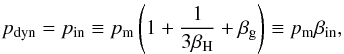 (1)where βin = 1 + 1/3βH + βg,
βH = ϵH/ϵr
is the ratio of the energies of magnetic field, ϵH, and all relativistic particles,
ϵr, βg = pg/pm.
A profile of the magnetic pressure pm along the jet is evaluated by using the
rest-frame spectral density of synchrotron radiation flux Sν (hereafter brightness),
assuming a power-law energy spectrum of the electrons (e.g. Ginzburg, 1979, p. 97), as follows:
(1)where βin = 1 + 1/3βH + βg,
βH = ϵH/ϵr
is the ratio of the energies of magnetic field, ϵH, and all relativistic particles,
ϵr, βg = pg/pm.
A profile of the magnetic pressure pm along the jet is evaluated by using the
rest-frame spectral density of synchrotron radiation flux Sν (hereafter brightness),
assuming a power-law energy spectrum of the electrons (e.g. Ginzburg, 1979, p. 97), as follows: 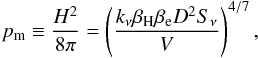 (2)where βe = ϵr/ϵe
is the ratio of the energy of all relativistic particles to the energy ϵe of relativistic
electrons, H is
the strength of the magnetic field, which is assumed to be randomly directed, and
V is the
volume of the radiating gas within the observing beam. The coefficient kν is 5.47 × 10¹⁷ in the case of SS 433:
the synchrotron spectral index is α = 0.74 (Sν ∝ ν−α),
the frequency ν = 4.86 GHz of the brightness profile Sν(r)
from Bell et al., (2011), and the frequency range
4.86–∞ GHz is accepted as the
whole range of the synchrotron spectrum of the relativistic electrons. The pressure
pm
may be underestimated by at most 2–3 times due to an uncertainty of the lower border of the
synchrotron spectrum.
(2)where βe = ϵr/ϵe
is the ratio of the energy of all relativistic particles to the energy ϵe of relativistic
electrons, H is
the strength of the magnetic field, which is assumed to be randomly directed, and
V is the
volume of the radiating gas within the observing beam. The coefficient kν is 5.47 × 10¹⁷ in the case of SS 433:
the synchrotron spectral index is α = 0.74 (Sν ∝ ν−α),
the frequency ν = 4.86 GHz of the brightness profile Sν(r)
from Bell et al., (2011), and the frequency range
4.86–∞ GHz is accepted as the
whole range of the synchrotron spectrum of the relativistic electrons. The pressure
pm
may be underestimated by at most 2–3 times due to an uncertainty of the lower border of the
synchrotron spectrum.
In our model, the magnetic field inside the jets and, therefore, the formation of the
synchrotron radiation are localized in the vicinity of dense clouds, in the cloud shells,
whose thickness lsh is approximately equal to a half the
size of the clouds, lcl, as Inoue et al., (2012) have demonstrated for clouds in supernova remnants. The
volume of these cloud shells per jet segment of unit length is 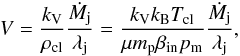 (3)where kV is the volume
ratio of the shells and clouds, ρcl = μmppcl/kBTcl
and Tcl the mass density and temperature of the
clouds, whose gas pressure pcl is assumed to be equal to the jet
average internal pressure pin = βinpm
(Eq. (1)), Ṁj is the flux of
the jet mass contained in the clouds, λj is the jet length per unit of
flight-time, μ
is the average relative molar mass of the clouds (≈ 0.6 for solar abundances), mp is the proton mass, and kB is the
Boltzmann constant. In the adopted case of spherical clouds, kV = (2lsh/lcl + 1)3 − 1.
After substituting the volume (3) and the
corresponding brightness per jet unit length, that is, the differential brightness
sν = dSν/dl
which depends on the jet length l, into Eq. (2), the latter is transformed into
(3)where kV is the volume
ratio of the shells and clouds, ρcl = μmppcl/kBTcl
and Tcl the mass density and temperature of the
clouds, whose gas pressure pcl is assumed to be equal to the jet
average internal pressure pin = βinpm
(Eq. (1)), Ṁj is the flux of
the jet mass contained in the clouds, λj is the jet length per unit of
flight-time, μ
is the average relative molar mass of the clouds (≈ 0.6 for solar abundances), mp is the proton mass, and kB is the
Boltzmann constant. In the adopted case of spherical clouds, kV = (2lsh/lcl + 1)3 − 1.
After substituting the volume (3) and the
corresponding brightness per jet unit length, that is, the differential brightness
sν = dSν/dl
which depends on the jet length l, into Eq. (2), the latter is transformed into 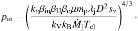 (4)The temperature of the
clouds in the SS 433 radio jets presumably increases downward of the jets, as suggested by
the observed X-ray brightening of the jets (Migliari et
al., 2002). In our model, the power-law profile Tcl(r) = T0rn
was adopted. Given the profiles of pressure and temperature, the distance of validity of the
model of the cloud thermodynamics is restricted by the following condition on the volume
filling of the jet by the clouds:
(4)The temperature of the
clouds in the SS 433 radio jets presumably increases downward of the jets, as suggested by
the observed X-ray brightening of the jets (Migliari et
al., 2002). In our model, the power-law profile Tcl(r) = T0rn
was adopted. Given the profiles of pressure and temperature, the distance of validity of the
model of the cloud thermodynamics is restricted by the following condition on the volume
filling of the jet by the clouds: 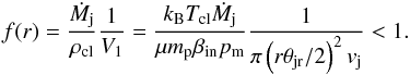 (5)Here, a conical
geometry of the jet is assumed, with the opening θjr, and the jet volume V1 per unit of
flight-time is approximated by the cylinder volume π(rθjr/2)2vj,
because the expansion of the jet is negligible: vj/r ≪ 1.
(5)Here, a conical
geometry of the jet is assumed, with the opening θjr, and the jet volume V1 per unit of
flight-time is approximated by the cylinder volume π(rθjr/2)2vj,
because the expansion of the jet is negligible: vj/r ≪ 1.
The extended radio jets do not show a helical pattern of the nutation, although there are
signs of the nutation of the radio jets within the brightening zone (Vermeulen et al., 1993; Mioduszewski
& Rupen, 2007). In the inner jets, the magnetic field is ordered and
aligned with the jet precession helix (Roberts et
al., 2008). Nutation would smear such order. All this suggests that the nutation
structure of the radio jets blurs with the distance r, and the jets acquire the
opening θjr = θj + θn = 68,
where
θj = 1
 2 and θn = 5
6 are the opening and the
nutation cone angle of the optical jets, respectively (Borisov & Fabrika, 1987). In this case, the angular velocity of the radio
jets is determined only by the precession, ω = 2π/Ppr,
and the azimuthal velocity is vφ = ωrsinθpr.
The length λj = |vj(r) − vφ(r) |
is determined by the vectors vj(r) and vφ(r) of the
jet radial and azimuthal velocities, respectively. In general, while the distance
r increases,
vj(r) deviates from the
ejection direction – hereafter the longitudinal Z-axis of the Cartesian rest-frame of reference of
the ballistic jet, with the azimuthal Y-axis chosen to be directed oppositely to the
precession movement, that is to vφ(r),
which is counterclockwise, viewed from the jet source (see Stirling et al., 2002, for a scheme of the jet precession and Fig. 1 for this frame of reference).
2 and θn = 5
6 are the opening and the
nutation cone angle of the optical jets, respectively (Borisov & Fabrika, 1987). In this case, the angular velocity of the radio
jets is determined only by the precession, ω = 2π/Ppr,
and the azimuthal velocity is vφ = ωrsinθpr.
The length λj = |vj(r) − vφ(r) |
is determined by the vectors vj(r) and vφ(r) of the
jet radial and azimuthal velocities, respectively. In general, while the distance
r increases,
vj(r) deviates from the
ejection direction – hereafter the longitudinal Z-axis of the Cartesian rest-frame of reference of
the ballistic jet, with the azimuthal Y-axis chosen to be directed oppositely to the
precession movement, that is to vφ(r),
which is counterclockwise, viewed from the jet source (see Stirling et al., 2002, for a scheme of the jet precession and Fig. 1 for this frame of reference).
The rest-frame brightness profile of the radio jet is approximated as 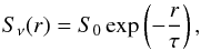 (6)with the brightness
Sν = 32.7 mJy per beam of
the telescope of a size
(6)with the brightness
Sν = 32.7 mJy per beam of
the telescope of a size  at ν = 4.86 GHz at the distance
 , and the
decrement
, and the
decrement  at the
flight-times t = 50–250d, where
at the
flight-times t = 50–250d, where  is the fiducial speed (Roberts et al., 2010; Bell
et al., 2011). Given expression (6)
for the brightness, the differential brightness will also be the exponential function
sν(r) = s0exp(−r/τ),
with the normalization factor
is the fiducial speed (Roberts et al., 2010; Bell
et al., 2011). Given expression (6)
for the brightness, the differential brightness will also be the exponential function
sν(r) = s0exp(−r/τ),
with the normalization factor 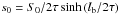 determined by Eq. (6) and the normalization
condition
determined by Eq. (6) and the normalization
condition  (7)where lb = φbD
is the linear size of the beam. The differential brightness sν(r)
grows exponentially upward of the jet at least to flight-times ~10d (Roberts et al., 2008). For shorter times, we extrapolated sν(r).
The differential brightness in dependency on the jet length is obtained from the condition
of conservation of sν(r)dr
when replacing the independent variable r by l, as sν(l) = sν(r)vj z(r)/λj(r),
where we replaced vj = dr/dt = vj xx/r + vj yy/r + vj zz/r
by the z-component of the jet velocity vj z(r) in the coordinate
system defined above, but with the axes origin at the source, because x,y ≪ z and
vj x,vj y ≪ vj z.
In the case of ballistic jets, we note that x,y,vj x,vj y = 0.
The transverse size of the jet projection onto the plane of the sky is smaller than the size
of the beam, and, hence, the definition of the differential brightness sν(r) of
the jet is valid at the flight-times < φbD/θjrvj ≈ 290d.
(7)where lb = φbD
is the linear size of the beam. The differential brightness sν(r)
grows exponentially upward of the jet at least to flight-times ~10d (Roberts et al., 2008). For shorter times, we extrapolated sν(r).
The differential brightness in dependency on the jet length is obtained from the condition
of conservation of sν(r)dr
when replacing the independent variable r by l, as sν(l) = sν(r)vj z(r)/λj(r),
where we replaced vj = dr/dt = vj xx/r + vj yy/r + vj zz/r
by the z-component of the jet velocity vj z(r) in the coordinate
system defined above, but with the axes origin at the source, because x,y ≪ z and
vj x,vj y ≪ vj z.
In the case of ballistic jets, we note that x,y,vj x,vj y = 0.
The transverse size of the jet projection onto the plane of the sky is smaller than the size
of the beam, and, hence, the definition of the differential brightness sν(r) of
the jet is valid at the flight-times < φbD/θjrvj ≈ 290d.
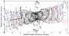 |
Fig. 1 Simulated loci of the radio jets of SS 433 for the settings vj/D = 0.2581c/4.8 kpc – the dynamic jet loci are marked by pluses every 20d of a flight, and the ballistic jet loci are marked by dots every 5d beginning from a flight-time of Ppr/2 – are superimposed on the image of the jets (courtesy of Dr. D.H. Roberts). Every simulated jet trace has a length of 800 flight days. The solid helical line is the ballistic jet loci drawn by Roberts et al., (2010) for the settings vj/D = 0.2647c/5.5 kpc. Approaching/receding parts of this helix are blue/red (in the on-line version of this paper). We show the longitudinal Z and azimuthal Y axes of the rest frame of reference of the ballistic jet of our simulation, with the axes origin located at a particular jet segment. The displacement vector between this segment and the segment of the same flight-time in the dynamic jet demonstrates the deviation of the kinematics of the dynamic jets from the ballistic kinematics. |
Now we have all constituents to write the equation of the dynamics 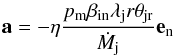 (8)of a jet
segment, independent of other segments, of the length λj, of the
transverse size rθjr, of the mass
Ṁj, which is under the dynamic pressure
pdyn = βinpm
(Eq. (1)). Here, η ≲ 1 is the geometrical
factor that characterizes the streamlining of the jet by swept-up gas and depending on the
transverse profile of the jet, and en is the unit vector of velocity of the jet
pattern relative to the ambient medium, which presumably is at rest. Equation (8), in fact an equation of the dynamics of the
material point, correctly describes the behaviour of a quasi-continuous precessing jet,
while the displacement of the jet from the ballistic (un-accelerated) position is relatively
small.
(8)of a jet
segment, independent of other segments, of the length λj, of the
transverse size rθjr, of the mass
Ṁj, which is under the dynamic pressure
pdyn = βinpm
(Eq. (1)). Here, η ≲ 1 is the geometrical
factor that characterizes the streamlining of the jet by swept-up gas and depending on the
transverse profile of the jet, and en is the unit vector of velocity of the jet
pattern relative to the ambient medium, which presumably is at rest. Equation (8), in fact an equation of the dynamics of the
material point, correctly describes the behaviour of a quasi-continuous precessing jet,
while the displacement of the jet from the ballistic (un-accelerated) position is relatively
small.
At angular distances beyond ~4′′, or t ~ 430d, the SS 433 radio jets look fragmentary (e.g. Roberts et al., 2010, Fig. 2) – likely the jets probably do not constitute a continuous stream and our model is not valid there.
3. Simulation of the dynamical jets of SS 433
The acceleration (8) was used to simulate the locus of the SS 433 jets. The initial conditions of this kinematic problem are defined by the standard kinematic model with the most accurate parameters to date collected in Table 1. A distance to SS 433 of 4.8 kpc was adopted, which is thought to be minimally biased by the acceleration (see above). This distance is possibly even smaller. The simulated locus was projected onto the plane of sky, accounting for the time delay of arriving photons to the observer that distorts image of the jets (the light travel effect).
Parameters of the standard kinematic model of the SS 433 jets.
The model jet loci are shown in Fig. 1 overplotted on
the deep image of the radio jets of SS 433 on July 11, 2003 from Roberts et al., (2010), where the jets are seen up to ~800 days of flight. The dynamic jets
simulated by our model with the settings vj/D = 0.2581c/4.8
kpc for the initial speed and distance, and the ballistic jets obtained by Roberts et al., (2010) for the settings vj/D = 0.2647c/5.5
kpc that were used by us as a template for the comparison, fit the observed radio jets
equally well: these two model loci are visually almost indistinguishable in both the inner
and external parts, the difference between them at a length 3′′ is lower than the accuracy of
 of the determination of the jet
ridge in this image reported by Blundell &
Bowler, (2004).
of the determination of the jet
ridge in this image reported by Blundell &
Bowler, (2004).
For the settings of the jet dynamics we chose the following characteristic values: a
geometry factor η = 1; a ratio lsh/lcl = 0.5
of the thickness of the radio bright shells around the jet clouds to the size of the clouds,
the finding of Inoue et al., (2012) for supernova
remnants; a pressure ratio of the thermal gas and magnetic field βg = 1, which is
expected in the vicinity of the jet clouds, where the magnetic field is amplified by the
shocks (Jones et al., 1996; Inoue et al., 2012); a ratio of the energy densities of the magnetic
field and relativistic particles βH = 3/4, which
corresponds minimum total energy of the field and particles (Ginzburg, 1979, p. 95); an initial flux of kinetic energy in the jet per cloud
fraction, 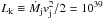 erg/s, and a
temperature of the jet clouds Tcl = 2 × 10⁴ K at a distance
of 1015 cm, which are
very tightly determined for the optical jet (Panferov
& Fabrika, 1997). The jet mass-flux Ṁj was assumed to
be constant throughout the jet length. Only two parameters were fitted: an exponent of the
cloud temperature profile
erg/s, and a
temperature of the jet clouds Tcl = 2 × 10⁴ K at a distance
of 1015 cm, which are
very tightly determined for the optical jet (Panferov
& Fabrika, 1997). The jet mass-flux Ṁj was assumed to
be constant throughout the jet length. Only two parameters were fitted: an exponent of the
cloud temperature profile  ,
which tunes the equality of goodness of the fits to the inner and extended jets, and a ratio
of the energies of all the relativistic particles and relativistic electrons βe = 2.7 ± 0.4,
although this is not an independent fitting parameter. The accuracies of the fitted
parameters correspond to a deviation of the dynamical jets from the template in Fig. 1 of half the image resolution
,
which tunes the equality of goodness of the fits to the inner and extended jets, and a ratio
of the energies of all the relativistic particles and relativistic electrons βe = 2.7 ± 0.4,
although this is not an independent fitting parameter. The accuracies of the fitted
parameters correspond to a deviation of the dynamical jets from the template in Fig. 1 of half the image resolution
 at distances of about
6′′, where the
helix of the eastern jet is still clearly discernible. These best dynamical parameters are
summarized in Table 2. In the simulations, the jet
dynamics was taken into account only in the region from the radio-brightening zone to a
distance t1 = 215d of flight where the
filling factor f tends to 1 and, as a result, the model of the jet dynamics becomes invalid.
at distances of about
6′′, where the
helix of the eastern jet is still clearly discernible. These best dynamical parameters are
summarized in Table 2. In the simulations, the jet
dynamics was taken into account only in the region from the radio-brightening zone to a
distance t1 = 215d of flight where the
filling factor f tends to 1 and, as a result, the model of the jet dynamics becomes invalid.
Dynamical parameters of the SS 433 jets.
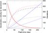 |
Fig. 2 Deviations of kinematical parameters of the dynamical jets from those of the ballistic jets in dependency on the flight-time. Along the left axis, thick and thin solid red lines: tangential deceleration aτ(t), in units of c/Ppr, and relative decrement δvj(t) of the jet velocity, respectively. Along the right axis, thick and thin dotted blue lines: transverse Δy(t) and longitudinal −Δz(t) deviations, respectively, of the dynamical jet loci in the comoving frame of reference of the ballistic jet, in units of mas; thick and thin dashed black lines: increment of azimuth Δψ(t) of the precession rotation, in units of a tenth of a degree, and increment Δθpr(t) of the precession cone semi-opening, in units of a hundredth of a degree, respectively. This figure is available in colour in the on line version of this paper. |
A deviation of the kinematics of the dynamic jets with the parameters given above from the
kinematics of the ballistic jets, with the same settings vj/D = 0.2581c/4.8
kpc, can be seen in Fig. 1 and is characterized in Fig.
2 by differences of the following kinematic
parameters in dependency on flight-time: tangential acceleration, velocity, coordinates
y and
z in the
frame of reference comoving with the ballistic jet, azimuthal angle of the precession
ψ, and
precession cone half-angle. The profile of deceleration
 ,
which is the length of the tangential component of the jet acceleration vector (8), shows a decrease of the deceleration downward
of the jets from a peak value of 0.081c/Ppr
in the radio-brightening zone, as Stirling et al.,
(2004) suggested. This means that the deceleration takes place mainly within the inner jets.
An average value of this deceleration in the first precession cycle is 0.019c/Ppr.
A full relative decrement of the jet speed is δvj ≡ 1 − vj(t1)/vj(0) = 7.5%,
half of this is accumulated at a distance of t1/2 = 33d,
that is, during one-fifth of the precession period. Approximately the same distance confines
the zone of significant slowdown of the jets: the jet-medium interaction beyond this
distance leads to a shift of the precession spiral at distances of about 6′′ no more than half of the image
resolution. Therefore, at t > Ppr
the external jets are expected be significantly ballistic. During a flight-time of
Ppr, or in bounds of
,
which is the length of the tangential component of the jet acceleration vector (8), shows a decrease of the deceleration downward
of the jets from a peak value of 0.081c/Ppr
in the radio-brightening zone, as Stirling et al.,
(2004) suggested. This means that the deceleration takes place mainly within the inner jets.
An average value of this deceleration in the first precession cycle is 0.019c/Ppr.
A full relative decrement of the jet speed is δvj ≡ 1 − vj(t1)/vj(0) = 7.5%,
half of this is accumulated at a distance of t1/2 = 33d,
that is, during one-fifth of the precession period. Approximately the same distance confines
the zone of significant slowdown of the jets: the jet-medium interaction beyond this
distance leads to a shift of the precession spiral at distances of about 6′′ no more than half of the image
resolution. Therefore, at t > Ppr
the external jets are expected be significantly ballistic. During a flight-time of
Ppr, or in bounds of
 from the jet source, the
precession cone semi-opening increases by Δθpr = 2
0, and the jet azimuth
increases by Δψ = 37° (that is, the precession phase 1 − ψ/2π decreases
by 0.10), or the jets become
offset along the azimuth direction by Δy = 316 milliarcsec (mas), which is approximately
2.6 times more than the
longitudinal offset | Δz| = 121 mas against the Z-axis (note that the
distance r
decreases by the lower value
from the jet source, the
precession cone semi-opening increases by Δθpr = 2
0, and the jet azimuth
increases by Δψ = 37° (that is, the precession phase 1 − ψ/2π decreases
by 0.10), or the jets become
offset along the azimuth direction by Δy = 316 milliarcsec (mas), which is approximately
2.6 times more than the
longitudinal offset | Δz| = 121 mas against the Z-axis (note that the
distance r
decreases by the lower value  mas) – the precession helix
shrinks along the precession axis and curls even more. This is expected to be detected as a
slowing-down and precession lag of the observed jets compared with the standard kinematic
model, although the curling is visually perceived merely as the shrinking and therefore
cannot be distinguished in the jet observations that not resolved in time. The average
visual slowdown of the dynamical jets, which is related to the distances difference
Δrvis between the segments of ballistic and
dynamic jets of the same azimuth, is 0.077c/Ppr
during the first precession cycle and 0.027c/Ppr
during a flight-time of 350d. The latter is higher than the value 0.02c/Ppr
found by Stirling et al., (2004) for approximately
the same flight-time. These authors also took note of the delay of the jets in precession
phase, by 0.25. A full visual
relative decrement of the jet velocity is δvj vis = Δrvis(t1)/t1vj(0) = 13%,
neglecting the deceleration.
mas) – the precession helix
shrinks along the precession axis and curls even more. This is expected to be detected as a
slowing-down and precession lag of the observed jets compared with the standard kinematic
model, although the curling is visually perceived merely as the shrinking and therefore
cannot be distinguished in the jet observations that not resolved in time. The average
visual slowdown of the dynamical jets, which is related to the distances difference
Δrvis between the segments of ballistic and
dynamic jets of the same azimuth, is 0.077c/Ppr
during the first precession cycle and 0.027c/Ppr
during a flight-time of 350d. The latter is higher than the value 0.02c/Ppr
found by Stirling et al., (2004) for approximately
the same flight-time. These authors also took note of the delay of the jets in precession
phase, by 0.25. A full visual
relative decrement of the jet velocity is δvj vis = Δrvis(t1)/t1vj(0) = 13%,
neglecting the deceleration.
4. Discussion
We found that the SS 433 radio jets must be under a considerable dynamical impact, if relativistic electrons responsible for the observed radiation are steadily injected by the shocks inside the jet, which are triggered by the shocks excited at the jet surface. In the collision with the ambient medium the jet acquires additional momentum whose vector lies in the tangential plane (YZ) to the precession cone and causes the jet to decelerate along the Z-axis and shift along the Y-axis. The acquired shift, demonstrated in Fig. 1 by the displacement vector, must be observed as an increase of torsion of the precession helix, or as a decrease of the precession phase. This might be the reason why the precession phase of every radio jet observation deviates from the kinematic model (Z. Paragi, 2009, priv. comm.). Note that the known azimuthal asymmetry of radiation of the optical jets points to a similar character of the jet-medium interaction (Panferov et al., 1997). If the collision occured at the front of the jet clouds, along the Z-axis, one would expect only a deceleration of the radio jets – in this case, the dynamical model fits the observed jets for no values of the dynamical parameters. The significant offset Δy of the dynamical jets allows us to explain the appearance of individual clouds outside of the SS 433 radio jet trace as a result of the uneven ram pressure of the inhomogeneous wind on the fragmented jets.
The dynamical model fits the radio jets of SS 433 well when the object is placed at a distance of 4.8 kpc. The deceleration is highest in the radio-brightening zone and decreases downward the jet. Accordingly, the strongest radio jet radiation is associated with the highest jet kinetic energy loss. The zone of the (significant) deceleration spans a flight-time of only one-fifth of the precession period. Beyond the deceleration zone the dynamical jets imitate ballistic jets with a speed 0.2647c and at the larger distance to the object 5.5 kpc. There are contradictory estimates of the distance (see Lockman et al., 2007, and references therein), including those obtained by the kinematic method on the basis of observations of the inner and extended radio jets. The dynamical model solves the dichotomy of the kinematic distance.
Blundell & Bowler, (2004) have fitted the extended radio jets by the ballistic model by allowing the jet speed to vary stochastically. The speed variation magnitude they found is 0.032c(4.8 kpc/5.5 kpc) = 0.028c, or ≈ 11% of the jet speed, within the parameters of our model, which is comparable with the visual relative decrement δvj vis = 13% issued from the jet dynamics. The observed speed variations may be partly due to uneven deceleration in the inner jets2. As for the distance to SS 433, the results of Blundell & Bowler, (2004) for the extended radio jets do not depend on the deceleration, which occures in the inner jets, nor exclude the dynamic model, which shows that the extended jets are ballistic with the parameters vj = 0.2387c and D = 4.8 kpc, which are intermediate to the two options they have discerned on the basis of the light travel effect.
It is quite possible that the blurring of the nutation structure of the jets occures within the deceleration zone, because the ram pressure on the jets, depending on the jet azimuthal velocity, is strongly modulated with nutation phase. In this case the jet velocity variations normal to the jet axis have to be of the order of ≳ θnvj ≈ 0.1vj – exactly the magnitude of the observed jet speed variations during the first 40 flight days (Schillemat et al., 2004). In addition, the blurring may be initiated by abrupt heat and expansion of the jet clouds and decollimation of the jets in the radio-brightening zone, where pressure in the jets probably decreases steeply (Vermeulen et al., 1993; Panferov, 1999). The lack of the nutation structure in the radio jets may also be a manifestation of the two-stream structure of the jets in the beginning: with the nutating central stream, observed in the optics, and the wider shell stream, which damps the nutation. Jets with this structure might arise in scenarios of the type described by Begelman et al., (2006).
The huge power loss of kinetic energy of the radio jet Ẇk ≈ 2δvjLk = 1.50 × 1038 erg/s is not observed radiatively. Possibly, this power is drained into mechanical energy of the wind that interacts with the jets, and is eventually transformed into mechanical energy of the W 50 shell (Dubner et al., 1998). Similarly, the high efficiency of the mechanical energy transfer from jets to atomic and molecular outflows in the surroundings is observed in AGNs (Morganti et al., 2013).
The model of the jet dynamics unites different properties of the SS 433 radio jets such as
the dynamics and radiation. The parameters of this model are not independent of each other
and may be subjected to transformations that do not change the found profile of the jet
acceleration, by the following formula: 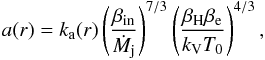 (9)obtained from (4) and (8), where
 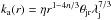 (kνμmpD2sν/kB)4/3.
The values of lsh/lcl,
βg, βH, βe,
Lk
and T0, given in Table 2 do not only provide the best fit of the dynamical model, but are also
justified observationally and theoretically, but may be βe, which in turn
validates the model. If we were to change the found suspiciously low value βe = 2.7 by 100,
the value observed near Earth (Ginzburg, 1979, p.
96), then Eq. (9), with the invariant
a(r), dictates the change of
Lk = 1 × 1039 erg/s by
7.9 × 1039 erg/s,
or lsh/lcl = 0.5
by 2.7, or Tcl(1015 cm) = 2 × 104
K by 7.4 × 105 K –
all of these are beyond the reasonable ranges. Similarly, the scope of the variations
allowed by Eq. (9) of another dynamical
parameter is severely restricted. There is a reserve for increase of βe in the
uncertainties of the parameters incorporated in ka(r): lowering of
η from the
accepted unlikely maximum (see Table 2),
sν by the off-jet fraction
of the emission (Roberts et al., 2008), and
kν due to the polarization
of the emission, in which case the magnetic field averaged over all directions is expected
to be weaker than in the case of the random field assumed in Eq. (2), all together could boost βe by about a
factor of 2.
(kνμmpD2sν/kB)4/3.
The values of lsh/lcl,
βg, βH, βe,
Lk
and T0, given in Table 2 do not only provide the best fit of the dynamical model, but are also
justified observationally and theoretically, but may be βe, which in turn
validates the model. If we were to change the found suspiciously low value βe = 2.7 by 100,
the value observed near Earth (Ginzburg, 1979, p.
96), then Eq. (9), with the invariant
a(r), dictates the change of
Lk = 1 × 1039 erg/s by
7.9 × 1039 erg/s,
or lsh/lcl = 0.5
by 2.7, or Tcl(1015 cm) = 2 × 104
K by 7.4 × 105 K –
all of these are beyond the reasonable ranges. Similarly, the scope of the variations
allowed by Eq. (9) of another dynamical
parameter is severely restricted. There is a reserve for increase of βe in the
uncertainties of the parameters incorporated in ka(r): lowering of
η from the
accepted unlikely maximum (see Table 2),
sν by the off-jet fraction
of the emission (Roberts et al., 2008), and
kν due to the polarization
of the emission, in which case the magnetic field averaged over all directions is expected
to be weaker than in the case of the random field assumed in Eq. (2), all together could boost βe by about a
factor of 2.
The density of the ambient medium, extracted from the dynamical model simulation by the
formula na = βinpm/ηmp(envj)2,
is shown in Fig. 3. This density is essentially lower
than the density niso ∝ Ṁw/vwr2
of the wind from the system’s accretion disk by several orders of value, if this wind is
isotropic – the jets propagate in almost empty channels in the wind. The exponent of the
power-law fit na ∝ t−m
to the profile in Fig. 3, ranging from ~4 to ~6 with flight-time, also shows the
anisotropy of the wind. It also shows the density ratio of the ambient medium to the jets –
it is essentially lower than 1 beyond the deceleration zone. The magnetic field in the
vicinity of the jet clouds is shown in Fig. 3,
conforming to the ram pressure by Eqs. (1),
(2). In the radio-brightening zone
( ), the magnetic field strength is
0.51 G which differs from the
0.08 G found by Vermeulen et al., (1987) because we accounted for the
clumping of the jets.
), the magnetic field strength is
0.51 G which differs from the
0.08 G found by Vermeulen et al., (1987) because we accounted for the
clumping of the jets.
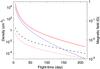 |
Fig. 3 Density of the ambient medium of the SS 433 jets (thick red line) and its ratios to the isotropic wind density (thin red line) and to the jets average density (dashed black line) are plotted along the left axis in dependency on flight-time. The strength of the magnetic field in the vicinity of the jet clouds (dotted blue line) is plotted along the right axis. This figure is available in colour in the online version of this paper. |
The volume-filling of the jets by the clouds increases with distance because the clouds are heated and expand as a result, while the cloud pressure, which is in balance with the jet internal pressure, is held by the ram pressure on the jets, which is falling. The cloud temperature rises from 1.4 × 10⁵ K in the brightening zone to 3.0 × 10⁷ K at the flight-times ~t1 = 215d where the filling f → 1 and the model becomes invalid. In fact, the jet kinematics is hardly sensitive to the dynamics prescribed by the model beyond the deceleration zone. Therefore, the cloud behaviour there, in particular the reheating, may be non-monotonic without violating our findings on the jet kinematics. Given the temperature increment ΔTcl, the power of jet heating is kBΔTcl(3Ṁj/2μmp) = 2.1 × 1035 erg/s, which is quite enough to provide the observed jet X-ray luminosity ~1033 erg/s and is surprisingly close to the radio jet synchrotron luminosity. All of this energy budget is minuscule in comparison with the power-loss of the jet kinetic energy 1.50 × 1038 erg/s – we are left with the puzzle where the latter is deposited.
Our simulation shows that the radio jets of SS 433 can be decelerating and twisting in addition to the precession twist. In this case, the arcsecond-scale jets imitate ballistic jets at an inappropriate distance from the observer. An explicit detection of the jet dynamics is a quest for future observations of the inner radio jets.
1′′ = 0.72 × 1017 cm at a distance of 4.8 kpc.
We also also note that in a patchy jet with an openning θjr = 6.8°, inclined to the line of sight by θ ≥ θi = i − θpr ≈ 59°, a natural spread of the apparent velocities of the patches Δvτ = Δ(vjsinθ) is on the order of Δvτ/vτ ≈ Δθcotθ ≤ θjrcotθi = 7.1%.
References
- Abell, G. O., & Margon, B. 1979, Nature, 279, 701 [NASA ADS] [CrossRef] [Google Scholar]
- Begelman, M. C., King, A. R., & Pringle, J. E. 2006, MNRAS, 370, 399 [NASA ADS] [CrossRef] [Google Scholar]
- Bell, M. R., Roberts, D. H., & Wardle, J. F. C. 2011, ApJ, 736, 118 [NASA ADS] [CrossRef] [Google Scholar]
- Blundell, K. M., & Bowler, M. G. 2004, ApJ, 616, L159 [NASA ADS] [CrossRef] [Google Scholar]
- Borisov, N. V., & Fabrika, S. N. 1987, Pis’ma v Astron. Zh., 13, 487 [NASA ADS] [Google Scholar]
- Brinkmann, W., Pratt, G. W., Rohr, S., Kawai, N., & Burwitz, V. 2007, A&A, 463, 611 [NASA ADS] [CrossRef] [EDP Sciences] [Google Scholar]
- Davydov, V. V., Esipov, V. F., & Cherepashchuk, A. M. 2008, Astron. Rep., 52, 487 [NASA ADS] [CrossRef] [Google Scholar]
- Dubner, G. M., Holdaway, M., Goss, W. M., & Mirabel, I. F. 1998, ApJ, 116, 1842 [Google Scholar]
- Fabrika, S. 2004, Astrophys. Space Phys. Rev., 12, 1 [NASA ADS] [Google Scholar]
- Fejes, I. 1986, A&A, 168, 69 [NASA ADS] [Google Scholar]
- Ginzburg, V. L. 1979, Theoretical Physics and Astrophysics (Oxford: Pergamon Press) [Google Scholar]
- Heavens, A. F., Ballard, K. R., & Kirk, J. G. 1990, MNRAS, 244, 474 [NASA ADS] [Google Scholar]
- Hjellming, R. M., & Johnston, K. J. 1981, ApJ, 246, L141 [NASA ADS] [CrossRef] [Google Scholar]
- Hjellming, R. M., & Johnston, K. J. 1988, ApJ, 328, 600 [NASA ADS] [CrossRef] [Google Scholar]
- Inoue, T., Yamazaki, R., Inutsuka, S.-I., & Fukui, Y. 2012, ApJ, 744, 71 [NASA ADS] [CrossRef] [Google Scholar]
- Jones, T. W., Ryu, D., & Tregillis, I. L. 1996, ApJ, 473, 365 [NASA ADS] [CrossRef] [Google Scholar]
- Kopylov, I. M., Kumaigorodskaja, R. N., & Somov, N. N. 1987, AZh, 64, 785 [NASA ADS] [Google Scholar]
- Kundt, W. 1987, Ap&SS, 134, 407 [NASA ADS] [CrossRef] [Google Scholar]
- Lockman, F. J., Blundell, K. M., & Goss, W. M. 2007, MNRAS, 381, 881 [NASA ADS] [CrossRef] [Google Scholar]
- Marshall, H. L., Canizares, C. R., & Schulz, N. S. 2002, ApJ, 564, 941 [NASA ADS] [CrossRef] [Google Scholar]
- Migliari, S., Fender, R., & Méndez, M. 2002, Science, 297, 1673 [NASA ADS] [CrossRef] [PubMed] [Google Scholar]
- Miller-Jones, J. C. A., Migliari, S., Fender, R. P., et al. 2008, ApJ, 682, 1141 [NASA ADS] [CrossRef] [Google Scholar]
- Mioduszewski, A. J., & Rupen, M. P. 2007, BAAS, 38, 954 [Google Scholar]
- Morganti, R., Frieswijk, W., Oonk, R. J. B., Oosterloo, T., & Tadhunter, C. 2013, A&A, 552, L4 [NASA ADS] [CrossRef] [EDP Sciences] [Google Scholar]
- Newsom, G. H., & Collins, G. W., II. 1981, AJ, 86, 1250 [NASA ADS] [CrossRef] [Google Scholar]
- Panferov, A. A. 1999, A&A, 351, 156 [NASA ADS] [Google Scholar]
- Panferov, A. A., & Fabrika, S. N. 1997, Astron. Rep., 41, 506 [NASA ADS] [Google Scholar]
- Panferov, A. A., Fabrika, S. N., & Rakhimov, V. Yu. 1997, Astron. Rep., 41, 342 [NASA ADS] [Google Scholar]
- Paragi, Z., Stirling, A. M., & Fejes, I. 2003, in 4th Microquasars Workshop, New Views on Microquasars, eds. Ph. Durouchoux, Y. Fuchs, & J. Rodriguez (Kolkata, India: Center for Space Physics), 288 [Google Scholar]
- Roberts, D. H., Wardle, J. F. C., Lipnick, S. L., Selesnick, P. L., & Slutsky, S. 2008, ApJ, 676, 584 [NASA ADS] [CrossRef] [Google Scholar]
- Roberts, D. H., Wardle, J. F. C., Bell, M. R., et al. 2010, ApJ, 719, 1918 [NASA ADS] [CrossRef] [Google Scholar]
- Romney, J. D., Schilizzi, R. T., Fejes, I., & Spencer, R. E. 1987, ApJ, 321, 822 [NASA ADS] [CrossRef] [Google Scholar]
- Schillemat, K., Mioduszewski, A., Dhawan, V., & Rupen, M. 2004, BAAS, 36, 1515 [NASA ADS] [Google Scholar]
- Spencer, R. E. 1984, MNRAS, 209, 869 [NASA ADS] [Google Scholar]
- Stirling, A. M., Jowett, F. H., Spencer, R. E., Paragi, Z., & Ogley, R. N. 2002, MNRAS, 337, 657 [NASA ADS] [CrossRef] [Google Scholar]
- Stirling, A. M., Spencer, R. E., Cawthorne, T. V., & Paragi, Z. 2004, MNRAS, 354, 1239 [NASA ADS] [CrossRef] [Google Scholar]
- Vermeulen, R. C., Schilizzi, R. T., Icke, V., Fejes, I., & Spencer, R. E. 1987, Nature, 328, 309 [NASA ADS] [CrossRef] [Google Scholar]
- Vermeulen, R. C., Schilizzi, R. T., Spencer, R. E., Romney, J. D., & Fejes, I. 1993, A&A, 270, 177 [NASA ADS] [Google Scholar]
All Tables
All Figures
|
Fig. 1 Simulated loci of the radio jets of SS 433 for the settings vj/D = 0.2581c/4.8 kpc – the dynamic jet loci are marked by pluses every 20d of a flight, and the ballistic jet loci are marked by dots every 5d beginning from a flight-time of Ppr/2 – are superimposed on the image of the jets (courtesy of Dr. D.H. Roberts). Every simulated jet trace has a length of 800 flight days. The solid helical line is the ballistic jet loci drawn by Roberts et al., (2010) for the settings vj/D = 0.2647c/5.5 kpc. Approaching/receding parts of this helix are blue/red (in the on-line version of this paper). We show the longitudinal Z and azimuthal Y axes of the rest frame of reference of the ballistic jet of our simulation, with the axes origin located at a particular jet segment. The displacement vector between this segment and the segment of the same flight-time in the dynamic jet demonstrates the deviation of the kinematics of the dynamic jets from the ballistic kinematics. |
| In the text | |
|
Fig. 2 Deviations of kinematical parameters of the dynamical jets from those of the ballistic jets in dependency on the flight-time. Along the left axis, thick and thin solid red lines: tangential deceleration aτ(t), in units of c/Ppr, and relative decrement δvj(t) of the jet velocity, respectively. Along the right axis, thick and thin dotted blue lines: transverse Δy(t) and longitudinal −Δz(t) deviations, respectively, of the dynamical jet loci in the comoving frame of reference of the ballistic jet, in units of mas; thick and thin dashed black lines: increment of azimuth Δψ(t) of the precession rotation, in units of a tenth of a degree, and increment Δθpr(t) of the precession cone semi-opening, in units of a hundredth of a degree, respectively. This figure is available in colour in the on line version of this paper. |
| In the text | |
|
Fig. 3 Density of the ambient medium of the SS 433 jets (thick red line) and its ratios to the isotropic wind density (thin red line) and to the jets average density (dashed black line) are plotted along the left axis in dependency on flight-time. The strength of the magnetic field in the vicinity of the jet clouds (dotted blue line) is plotted along the right axis. This figure is available in colour in the online version of this paper. |
| In the text | |
Current usage metrics show cumulative count of Article Views (full-text article views including HTML views, PDF and ePub downloads, according to the available data) and Abstracts Views on Vision4Press platform.
Data correspond to usage on the plateform after 2015. The current usage metrics is available 48-96 hours after online publication and is updated daily on week days.
Initial download of the metrics may take a while.