| Issue |
A&A
Volume 562, February 2014
|
|
|---|---|---|
| Article Number | A57 | |
| Number of page(s) | 11 | |
| Section | The Sun | |
| DOI | https://doi.org/10.1051/0004-6361/201322263 | |
| Published online | 05 February 2014 | |
Plasma radio emission from inhomogeneous collisional plasma of a flaring loop
1 Centre for Space, Fusion and Astrophysics, University of Warwick, CV4 7AL, UK
e-mail: This email address is being protected from spambots. You need JavaScript enabled to view it.
2 School of Physics & Astronomy, University of Glasgow, G12 8QQ, UK
Received: 11 July 2013
Accepted: 5 December 2013
Abstract
The evolution of a solar flare accelerated non-thermal electron population and associated plasma emission is considered in collisional inhomogeneous plasma. Non-thermal electrons collisionally evolve to become unstable and generate Langmuir waves, which may lead to intense radio emission. We self-consistently simulated the collisional relaxation of electrons, wave-particle interactions, and non-linear Langmuir wave evolution in plasma with density fluctuations. Additionally, we simulated the scattering, decay, and coalescence of the Langmuir waves which produce radio emission at the fundamental or the harmonic of the plasma frequency, using an angle-averaged emission model. Long-wavelength density fluctuations, such as are observed in the corona, are seen to strongly suppress the levels of radio emission, meaning that a high level of Langmuir waves can be present without visible radio emission. Additionally, in homogeneous plasma, the emission shows time and frequency variations that could be smoothed out by density inhomogeneities.
Key words: Sun: particle emission / Sun: radio radiation / Sun: flares
© ESO, 2014
1. Introduction
During solar flares, efficient acceleration of electrons in coronal loops is often observed. Such non-thermal electrons produce several radiation signatures, in particular hard X-rays (HXR), and radio emissions. These signatures are a valuable diagnostic for the properties of non-thermal electron populations. HXR emission is produced by collisional bremsstrahlung in the dense plasma of loop footpoints, and is particularly useful because the coronal plasma is optically thin to these wavelengths, and the cross-section for emission well known. Gyrosynchrotron emission (gyroemission from mildly relativistic particles) can produce strong continuum radio emission at GHz frequencies in regions of high magnetic field, while coherent emission mechanisms can produce intense radio bursts in some circumstances.
In particular, as noted by Emslie & Smith (1984), Hamilton & Petrosian (1987) fast electrons in dense plasma can produce Langmuir wave turbulence because of collisional evolution, and this can lead to intense plasma radio emission due to the large number of non-thermal electrons in flares. This collisional relaxation is the mechanism we consider here. For emission at the harmonic of the plasma frequency, resulting from the coalescence of two counter propagating Langmuir waves, a simple analytical estimate shows that this process should saturate at a brightness temperature equal to the brightness temperature of the Langmuir waves, therefore often reaching several orders of magnitude over the thermal level and thus easily visible.
On the other hand, Langmuir waves are known to be strongly affected by fluctuations in plasma density. Spreading of Langmuir waves in angle because of elastic scattering by density fluctuations was considered by e.g. Nishikawa & Ryutov (1976) and Muschietti et al. (1985) and found to suppress the beam-plasma interaction. A similar result for beam-aligned density fluctuations was found in our previous work (Ratcliffe et al. 2012). Moreover, Langmuir waves generated in non-uniform plasma can be shifted to lower wave numbers (higher phase velocities) and re-absorbed, leading to efficient acceleration of the tail of energetic electrons. A relatively high level of Langmuir waves can strongly affect the electron distribution above ~20 keV and lead to substantial over-estimation of electron number and energy in flares when simple collisional relaxation is assumed (Kontar et al. 2012). This self-acceleration of the electron tail is particularly efficient when the timescale of Langmuir wave refraction is similar to the timescale of Langmuir wave generation (Ratcliffe et al. 2012) and is evident in 3D PIC simulations in magnetised plasma (Karlický & Kontar 2012).
Thus it appears that density fluctuations can suppress the Langmuir wave generation from an electron population, and therefore allow for the existence of fast electrons without plasma radio emission. However, it still remains unclear whether a high level of Langmuir turbulence necessitates strong plasma emission in collisional flaring plasma, since a density gradient acting on Langmuir waves has already been found by Kontar & Pécseli (2002) to suppress Langmuir wave decay, potentially allowing the production of Langmuir waves without their conversion into radio emission. Addressing this problem requires detailed numerical simulations, because although the processes involved in the emission are qualitatively known (e.g. Ginzburg & Zhelezniakov 1958; Sturrock 1964; Zheleznyakov & Zaitsev 1970), an analytical treatment is not possible. Such numerical simulations are often employed for calculations applied to type III bursts (e.g. Li et al. 2008; Tsiklauri 2011).
Here we consider the plasma emission from accelerated electrons in a dense coronal loop. We self-consistently solve the problem of relaxation of a non-thermal electron population taking Langmuir wave excitation, absorption, and weakly-nonlinear evolution into account. We show that plasma emission will be produced at both the fundamental and the harmonic of the plasma frequency, reaching brightness temperatures up to several orders of magnitude above thermal, although due to the effects of escape through the surrounding plasma, only the harmonic component can be observed. The emission has an intrinsic bandwidth of the order of 5% of the plasma frequency due to its wavenumber spread and the dispersive nature of electromagnetic waves in plasma. In homogeneous density plasma, this emission shows significant time and frequency variations, while the presence of density fluctuations in the background plasma is seen to both smooth out these variations and reduce the brightness of the emission. A relatively modest level of density fluctuations is able to completely suppress the emission, despite the presence of a high level of Langmuir waves, while simultaneously producing electron self-acceleration and thus increasing the number of electrons at high velocities.
2. A model for electron and Langmuir wave evolution, and plasma radio emission
We consider a dense coronal loop embedded in the coronal plasma, as shown in Fig. 1. The electron density is the combination of a constant density background plus small magnitude, long wavelength random density fluctuations. The evolution of a non-thermal electron population is considered in the collisional region, with the electron distribution, and all wave distributions, assumed not to depend on position within the source volume. The electron beam-plasma system is self-consistently treated taking into account the effects of non-uniform plasma density, plasma collisionality, non-linear wave-wave processes and the production of electromagnetic radio emission near the plasma frequency and its harmonic.
All of these processes are interrelated, and therefore simulated simultaneously. The equations describing the evolution of the electron distribution are given in Sect. 2.1, and those for Langmuir waves and ion-sound waves in Sects. 2.2 and 2.3 respectively. The basic equations for electromagnetic emission are in Sect. 2.4, with the emission at the fundamental of the plasma frequency treated in Sect. 2.5, and the harmonic in Sect. 2.6. Finally, Sect. 2.7 addresses the considerations of propagation and absorption of electromagnetic emission. We note that the dynamics of electrons, Langmuir waves and ion-sound waves produced from Langmuir wave decay are all approximately one-dimensional. On the other hand, the equations for Langmuir wave conversion into electromagnetic emission are not, and are treated here using an angle-averaged approximation, described briefly below.
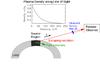 |
Fig. 1 Geometry of a model coronal loop. Within the loop the plasma density is approximately ne, with superimposed weak random density fluctuations. A fast electron population is produced in the source region, shaded dark grey, which relaxes collisionally, producing Langmuir waves and thus radio emission. Radio emission arises from the source region of linear size d ≃ 109 cm measured perpendicular to the loop axis, of the order of the typical cross-sectional size of a coronal loop. An observer at 1 AU sees a source with angular radius θ. The surrounding plasma has an exponential density profile of scale height H. |
2.1. Non-thermal electron evolution
We describe the electrons using their distribution function f(v,t) [cm-3/(cm s-1)], which is normalised so that 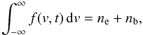 (1)where ne the density of the background plasma, and nb that of non-thermal electrons, and the Langmuir waves by their spectral energy density as a function of wavenumber k, W(k,t) [erg cm-2], where
 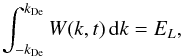 (2)is the total energy density of the waves in erg cm-3 and kDe = ωpe/vTe with
  the electron thermal velocity and
  the plasma frequency, and me,e the mass and charge of an electron respectively.
The equation for the evolution of the electron distribution is based on that in (Drummond & Pines 1964; Vedenov et al. 1962) with additional terms describing the effects of collisions. We have 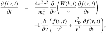 (3)with
 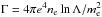 and lnΛ the Coulomb logarithm, approximately 20 in the solar corona.
The first term on the RHS of this equation describes emission and absorption of Langmuir waves by the electrons (Drummond & Pines 1964; Vedenov et al. 1962; Vedenov 1963). This is a resonant interaction between electrons and Langmuir waves, ωpe = kv1, i.e. the Langmuir wave phase velocity must equal the electron velocity. The second and third terms on the RHS describe collisional interaction of electrons with Maxwellian plasma (e.g. Lifshitz & Pitaevskii 1981): the second is the total energy loss and the third term accounts for the finite temperature of the background electrons. When the level of plasma waves is near thermal, the first term on the RHS becomes negligible and the stationary (∂f/∂t = 0) Maxwellian distribution is formed by collisions, i.e. by the second and the third terms. This collisional operator is approximately proportional to 1/v3 and so the slower electrons will lose energy more rapidly than the faster ones, leading to a reverse slope in velocity space, which will lead to generation of Langmuir waves. Langmuir wave generation will tend to flatten this reverse slope, while collisions continue to restore it, leading to a plateau in the electron distribution with slowly decreasing height as the electrons thermalise.
2.2. Langmuir wave evolution
The electron beam generates Langmuir waves (denoted L) with wavenumbers parallel to the direction of propagation. These may then be backscattered by two processes L ⇄ L′ + s involving ion-sound waves (denoted s) and L + i ⇄ L′ + i′ where i,i′ denote initial and final states of a plasma ion. The relative importance of these two processes depends strongly on the ratio of electron and ion temperatures, Te/Ti, which can vary between ~2 and 0.1 in the corona and solar wind (e.g. Gurnett et al. 1979; Newbury et al. 1998). Generally, ion scattering is important in plasma with Ti ≥ Te, where ion-sound waves are very strongly damped, and the decay involving ion-sound waves when the ion temperature is lower (e.g. Cairns 2000).
The governing equation for the spectral energy density of Langmuir waves is (Drummond & Pines 1964; Vedenov et al. 1962; Zheleznyakov & Zaitsev 1970)  (4)where
  , and k = ωpe/v. The first and second terms on the RHS are the spontaneous and stimulated emission of Langmuir waves by electrons. These terms are derived in the weak-turbulence limit,
  (5)so that the energy density of Langmuir waves is much less than the energy density of surrounding plasma.
Collisional damping of Langmuir waves (e.g. Lifshitz & Pitaevskii 1981; Melrose 1980a) is given by the third term on the RHS in Eq. (4), while the fourth describes Langmuir wave diffusion in wavenumber space due to long-wavelength plasma density fluctuations. For a plasma density which is given by  , the sum of a background and small fluctuations
  with length scales far larger than the Debye length, the diffusion coefficient is (Ratcliffe et al. 2012)
  (6)for random density fluctuations with characteristic velocity v0, wavenumber q0 and RMS (root mean square) fluctuation level
  , and
, and  the group velocity of Langmuir waves.
The two terms labelled St describe the scattering and decay of Langmuir waves by the processes L + i ⇄ L′ + i′ and L ⇄ L′ + s where i,i′ are an initial and scattered plasma ion and s denotes an ion-sound wave. Both of these produce back-scattered (negative wavenumber) Langmuir waves. The general expressions describing these processes are standard (e.g. Melrose 1980b; Tsytovich 1995), and have been rewritten here under the assumption that fast-electron generated Langmuir waves propagate approximately parallel to the generating electrons and therefore the ambient magnetic field. Hereafter, we omit the explicit time dependence of the spectral energy densities for clarity of notation.
Langmuir wave scattering by ions is described by ![Mathematical equation: \begin{eqnarray} \label{eqn:LIonA} {\rm St}_{\rm ion}(W(k))&= & \int {\rm d}k_{L'} \frac{\alpha_{\rm ion}}{|k-k_{L'}|} \exp{\left(-\frac{(\omega_L-\omega_{L'})^2}{2|k-k_{L'}|^2 {v}_{\rm Ti}^2}\right)} \notag \\&&\times\left[\frac{1}{k_{\rm B}T_{\rm i}}\frac{\omega_{L'}-\omega_L}{\omega_L}W(k_{L'})W(k)\right] \end{eqnarray}](/articles/aa/full_html/2014/02/aa22263-13/aa22263-13-eq44.png) (7)where k,kL′,ωL,ωL′ are the wavenumber and frequency of the initial and scattered Langmuir waves, and
(7)where k,kL′,ωL,ωL′ are the wavenumber and frequency of the initial and scattered Langmuir waves, and  (8)with \begin{lxirformule}${v}_{\rm Ti}=\sqrt{k_{\rm B} T_{\rm i}/M_{\rm i}}$\end{lxirformule} the ion thermal speed, and Mi the mass of a plasma ion. It is evident from the exponential factor that the scattering is strongest for ωL ≃ ωL′ and kL′ ≃ − k, i.e. for backscattering of the waves. The resulting momentum change for the Langmuir wave is absorbed by the ions which we assume to have a Maxwellian distribution at temperature Ti. This momentum transfer is small, so the deviation of the ion distribution from thermal can be neglected (Tsytovich 1995).
The second source term describes Langmuir wave decay, and is given by
![Mathematical equation: \begin{eqnarray} \label{eqn:4ql_sSrc} &&{\rm St}_{\rm decay}(W(k))=\alpha_S\omega_{k} \int {\rm d}k_S \omega_{k_S}^S \notag \\ &&\hspace*{4mm} \times\Biggl[ \left( \frac{W(k_L)}{\omega^L_{k_L}}\frac{W_S(k_S)}{\omega^S_{k_S}}- \frac{W(k)}{\omega^L_k}\left(\frac{W(k_L)}{\omega^L_{k_L}}+ \frac{W_S(k_S)}{\omega^S_{k_S}}\right)\right)\notag\\&&\hspace*{4mm}\times\delta (\omega^L_{k}-\omega^L_{k_L}-\omega^S_{k_S})\Biggr. \notag \\&& \hspace*{4mm}-\left. \left( \frac{W(k_{L'})}{\omega^L_{k_{L'}}}\frac{W_S(k_S)}{\omega^S_{k_S}}- \frac{W(k)}{\omega^L_k}\left(\frac{W(k_{L'})}{\omega^L_{k_{L'}}}- \frac{W_S(k_S)}{\omega^S_{k_s}}\right)\right)\right.\notag \\ &&\hspace*{4mm}\times \Biggl.\delta(\omega^L_{k}-\omega^L_{k_{L'}}+\omega^S_{k_S}) \Biggr], \end{eqnarray}](/articles/aa/full_html/2014/02/aa22263-13/aa22263-13-eq51.png) (9)where
(9)where  are the spectral energy density and frequency of ion-sound waves, given by
  with
with  the sound speed, and the constant is
  (10)For a given initial Langmuir wavenumber, k, we have two possible processes, namely L → L′ + s and L + s → L′. The wavenumbers of the resulting Langmuir wave, kL,kL′ respectively, and the participating ion-sound wave, kS, are found from simultaneous solution of the equations of energy conservation (encoded by the delta functions in Eq. (9)), and momentum conservation, given by kL = k − kS and kL′ = k + kS for the two processes respectively. For example, for the process L → L′ + s we find kL ≃ − k, and kS ≃ 2k, and the initial Langmuir wave is backscattered. More precisely, we have kL = −k + Δk with the small increment
  . Thus repeated scatterings tend to accumulate Langmuir waves at small wavenumbers.
2.3. Ion-sound wave evolution
The evolution of the ion-sound wave distribution is given by (e.g. Melrose 1980b; Tsytovich 1995) 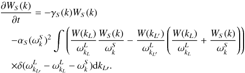 (11)The second term here is analogous to Eq. (9), describing the interaction of an ion-sound wave at wavenumber k with a Langmuir wave at wavenumber kL, producing a Langmuir wave at wavenumber kL′. Again, these participating wavenumbers are found from simultaneous solution of energy (frequency) and momentum (wavenumber) conservation. The first term is Landau damping of the waves, with coefficient
 ![Mathematical equation: \begin{equation} \gamma_S(k)=\sqrt{\frac{\pi}{2}}\omega^S_k\left[\frac{{v}_s}{{v}_{\rm Te}}+\left(\frac{{v}_s}{{v}_{\rm Ti}}\right)^3\exp\left[- \left(\frac{{v}_s^2}{2{v}_{\rm Ti}^2 }\right) \right]\right]\cdot \end{equation}](/articles/aa/full_html/2014/02/aa22263-13/aa22263-13-eq69.png) (12)Using the definitions of vs,vTe,vTi, we see that the ion contribution dominates and
(12)Using the definitions of vs,vTe,vTi, we see that the ion contribution dominates and ![Mathematical equation: \hbox{$\gamma_s\simeq \omega_k^S (3 + T_{\rm e}/T_{\rm i} )^{3/2}\exp{(-[3 + T_{\rm e}/T_{\rm i}])}$}](/articles/aa/full_html/2014/02/aa22263-13/aa22263-13-eq71.png) , which is of the order of
, which is of the order of  unless Ti ≪ Te, which is therefore a condition leading to high levels of ion-sound waves.
2.4. Electromagnetic emission
We describe the radio emission in terms of its brightness temperature, TT, which is defined from the Rayleigh-Jeans law for the radiation intensity as function of frequency by I(ν) = 2ν2kBTT/c2. We consider radiation at positive and negative wavenumber, the former propagating outwards from the Sun, along the direction of the beam propagation and the latter propagating backwards, and thus consider brightness temperature averaged over the corresponding hemisphere.
For thermal radiation, the definition of the brightness temperature gives TT = Te the plasma temperature. This radiation level is maintained by the thermal bremsstrahlung emission from the plasma particles, and by a corresponding damping. Kirchoff’s law says that these must be related by P(k) = γdTe for P the thermal emission rate, and γd the damping, in order that the two balance to give the thermal radiation level. Thus, from the bremsstrahlung damping rate,  (13)we can derive the thermal emission rate, or vice versa.
For emission described in terms of its brightness temperature we therefore have simply 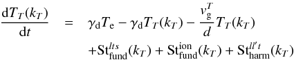 (14)where the first term is the thermal emission rate and the second term is the collisional damping. The third term, in which
  is the group velocity for electromagnetic waves, given by
  , and d is the source region size, describes the escape of radiation from the source region using a simple “leaky box” model. The waves propagate at velocity and so over a time dt, we will lose a fraction given by
  from the source region. Finally, we have the source terms, describing the production of radio emission from Langmuir waves, either at the fundamental, near ωpe or the harmonic near 2ωpe. These are derived in the following two subsections.
2.5. Fundamental electromagnetic source terms
The processes for emission at the fundamental are L ⇄ t ± s where L,s are Langmuir and ion-sound waves, and t is an EM wave, and L + i ⇄ t + i′, for i,i′ an initial and scattered plasma ion. The probability of both processes (e.g. Tsytovich 1995) is maximised for an EM wave with wavevector perpendicular to the initial Langmuir wave. Assuming the beam-generated Langmuir waves have some small angular spread in wavenumber space, covering a solid angle of ΔΩ, and further assuming that they are uniform within this spread, fundamental emission will be produced approximately isotropically. The larger the solid angle ΔΩ, the better this assumption becomes.
The source term entering Eq. (14) for fundamental emission by the processes L + s ⇄ t and L ⇄ t + s is again based on the general expressions in (e.g. Melrose 1980b; Tsytovich 1995). Rewriting in terms of the hemisphere-averaged brightness temperature, given by  (15)for WT(kT) the EM wave spectral energy density, and using the assumptions described in the previous paragraph gives
 ![Mathematical equation: \begin{eqnarray} \label{eqn:FundS} &&\mathrm{St}_{\rm fund}^{lts}(k_T)=\frac{\pi \omega_{\rm pe}^4{v}_s\left(1+\frac{3T_{\rm i}}{T_{\rm e}}\right)}{ 24 {v}_{\rm Te}^2n_{\rm e}T_{\rm e}} \times \int {\rm d}k_L \notag \\ &&\left\{ \left[\frac{W_S(k_S)}{\omega_{k_S}^S} \frac{2\pi^2}{ k_{\rm B} k_L^2\Delta\Omega} \frac{W_L({k}_L)}{\omega_{k_L}^L}-\frac{T_T({k}_T)}{\omega_{k_T}^T}\left( \frac{ W_S(k_S)}{\omega_{k_S}^S} + \frac{W_L(k_L)}{\omega_{k_L}^L}\right)\right]\right. \notag \\ && \hspace*{2.2mm} \times\delta(\omega_{k_L}^L +\omega_{k_S}^S-\omega_{k_T}^T) \notag\\\ &&\left.\hspace*{2.2mm} + \left[\frac{W_S(k_{S'})}{\omega_{k_{S'}}^S} \frac{2\pi^2}{k_{\rm B} k_L^2\Delta\Omega} \frac{W_L({k}_L)}{\omega_{k_L}^L}-\frac{T_T({k}_T)}{\omega_{k_T}^T}\left( \frac{ W_S(k_{S'})}{\omega_{k_{S'}}^S} - \frac{W_L(k_L)}{\omega_{k_L}^L}\right)\right]\right.\notag \\&&\left.\hspace*{2.2mm} \times\delta(\omega_{k_L}^L -\omega_{k_{S'}}^S-\omega_{k_T}^T)\right\}, \end{eqnarray}](/articles/aa/full_html/2014/02/aa22263-13/aa22263-13-eq97.png) (16)where the participating wavenumbers are obtained from energy and momentum conservation. However, in this case the momentum conservation condition must be obtained from the 3D description of the process. Using our assumption that the EM emission occurs approximately perpendicular to the initial Langmuir wave, the wavenumbers kL,kS,kT form a right-triangle and thus we find that
(16)where the participating wavenumbers are obtained from energy and momentum conservation. However, in this case the momentum conservation condition must be obtained from the 3D description of the process. Using our assumption that the EM emission occurs approximately perpendicular to the initial Langmuir wave, the wavenumbers kL,kS,kT form a right-triangle and thus we find that  .
.
Similarly, direct ion scattering, L + i ⇄ t + i′, is described by ![Mathematical equation: \begin{eqnarray} \label{eqn:FundIon} && \mathrm{St}_{\rm fund}^{ion}(k_T)=\int {\mathrm d} k_L \frac{\sqrt{\pi} \omega_{\rm pe}^2}{4 k_L n_{\rm e} {v}_{\rm Ti} (1+T_{\rm e}/T_{\rm i})^2} \exp{\left(-\frac{(\omega^T_{k_T}-\omega^L_{k_L})^2}{2k_L^2 {v}_{\rm Ti}^2}\right)} \notag\\&&\times\left[\frac{\omega^T_{k_T}}{\omega^L_{k_L}}\frac{2\pi^2W_L(k_L)}{ k_{\rm B} k_L^2}-T_T(k_T)-\frac{(2\pi)^3}{k_{\rm B} T_{\rm i}}\frac{\omega^T_{k_T}-\omega^L_{k_L}}{\omega^L_{k_L}}\frac{T_T(k_T)W_L(k_L)}{\Delta\Omega k_L^2}\right], \end{eqnarray}](/articles/aa/full_html/2014/02/aa22263-13/aa22263-13-eq101.png) (17)where again ΔΩ is the angular spread of the Langmuir waves, and we have assumed again that the EM emission occurs approximately perpendicular to the initial Langmuir wave. The momentum change between initial and final waves is absorbed by the plasma ions, which are assumed to be thermal, as in the case of Langmuir wave scattering by ions considered above.
(17)where again ΔΩ is the angular spread of the Langmuir waves, and we have assumed again that the EM emission occurs approximately perpendicular to the initial Langmuir wave. The momentum change between initial and final waves is absorbed by the plasma ions, which are assumed to be thermal, as in the case of Langmuir wave scattering by ions considered above.
2.6. Harmonic electromagnetic emission source terms
Emission at the harmonic of the plasma frequency occurs due to the coalescence of two Langmuir waves, L + L′ ⇄ t. Calculating an angle-averaged emission probability is complicated, because the emission probability depends directly on the participating wavenumbers, k1,k2 for the Langmuir waves, and kT for the EM wave, and the magnitudes of these depend on the geometry of the coalescence. In early models of emission, the “head-on-approximation” (HOA), where the Langmuir waves are almost antiparallel was suggested, which allows the emission probability to be greatly simplified. However, this assumption leads to significant overestimates of the emission rate, particularly at small wavenumbers (e.g. Melrose & Stenhouse 1979), as it assumes that the product electromagnetic wavenumber is far smaller than the initial Langmuir wavenumber, kT ≪ kL, whereas in fact  which is often comparable to kL.
Therefore the Langmuir waves cannot coalesce exactly head on, but rather at an angle less than π. Rather than specify this angle, which will depend on the values of kL and kT, we specify the angle between one of the initial Langmuir waves and the final EM wave. The emission probability is quadrupolar (Tsytovich 1970), with a maximum when this angle is π/4, assuming both waves have the same sign for the beam-parallel-component. We therefore use this value to solve the wavenumber and frequency matching equations. We then average the probability over its FWHM using these wavenumber values. For Langmuir waves which are uniform over a solid angle (in wavenumber space) of ΔΩ ≳ π/20 and for ωEM ≳ 2.01ωpe, the majority of Langmuir waves can participate in coalescence with the specified geometry, and we have an accurate approximation to the angle-averaged emission rate.
As in the case of fundamental emission, we use the general expressions of (e.g. Melrose 1980b; Tsytovich 1995), convert to brightness temperature using Eq. (15), and use our assumed emission geometry. The resulting source term for harmonic emission is ![Mathematical equation: \begin{eqnarray} &&\mathrm{St}_{\rm harm}^{ll't}(k_T) =\omega_{k_T}^T \frac{\pi \omega_{\rm pe}^2}{48 m_{\rm e} n_{\rm e} {v}_{\rm Te}^2} \int {\rm d} k_1 \frac{(k_2^2-k_1^2)^2}{4 k_2^2} \notag \\ && \hspace*{2.5mm}\times \left[\frac{2\pi^2}{k_{\rm B} k_2^2 \Delta\Omega}\frac{W(k_1)}{\omega_{k_1^L}}\frac{W(k_2)}{\omega_{k_2}^L}-\frac{T_T(k_T)}{\omega_{k_T}^T} \left(\frac{W(k_1)}{\omega_{k_1}^L}+\frac{W(k_2)}{\omega_{k_2}^L}\right)\right] \notag \\&&\hspace*{2.5mm} \times\delta(\omega_{k_1}+\omega_{k_2}-\omega_{k_T}^T), \end{eqnarray}](/articles/aa/full_html/2014/02/aa22263-13/aa22263-13-eq111.png) (18)where k1,k2 are the wavenumbers of the forwards and backwards coalescing Langmuir waves respectively, ωk1,ωk2 the corresponding Langmuir wave frequencies, and
(18)where k1,k2 are the wavenumbers of the forwards and backwards coalescing Langmuir waves respectively, ωk1,ωk2 the corresponding Langmuir wave frequencies, and  the wavenumber and frequency of the EM wave. From energy and momentum conservation, described by the delta function and by k1 + k2 = kT respectively, we have the conditions
  (19)considering only terms up to second order in kT, and using that ωT ≃ 2ωpe; and
  under the angular assumptions described previously.
2.7. Propagation and absorption of radio emission
Finally, to relate the brightness temperature of radio emission within the source, given by the solution of Eq. (14), to the observed flux we must consider the absorption of radiation during propagation. Collisional absorption (inverse bremsstrahlung) with damping rate γd gives an optical depth of  (20)where
  is the group velocity for electromagnetic waves. Because this tends to zero as ω tends to ωpe, emission at the fundamental has a far larger optical depth than that at the harmonic.
For emission at a frequency ω0 we then have  (21)We assume isothermal plasma between source and observer, with an exponential density profile ne(x) = n0exp( − x/H), where x is the distance from the region of emission at density n0, and H is the density scale height. The local plasma frequency is thus
  (22)From Eq. (21) we find
  (23)This may be integrated to find
 ![Mathematical equation: \begin{eqnarray} \label{eqn:optDepFin} \tau(\omega_0)&= &\sqrt{\frac{2}{\pi}}\frac{e^2 \ln\Lambda}{3 {v}_{\rm Te}^3 m_{\rm e}}\frac{H}{ c} \notag\\&&\times\left[ \omega_0^2 - \frac{1}{\omega_0}\sqrt{(\omega_0^2-\omega_{\rm pe}^2(0))}\left(\omega_0^2 +0.5\omega_{\rm pe}^2(0) \right) \right], \end{eqnarray}](/articles/aa/full_html/2014/02/aa22263-13/aa22263-13-eq128.png) (24)where we have neglected the small term involving plasma frequency at 1 AU.
(24)where we have neglected the small term involving plasma frequency at 1 AU.
The resulting escape fraction exp( − τ) is rather small for ωpe/(2π) ~ 1 GHz, and very dependent on the density scale height, H, chosen. For the corona this is around 109 cm which gives a fraction of around 1/50 for harmonic emission, and below 10-7 for the fundamental. A scale height of 6 × 108 cm gives again a very small result for the fundamental, and a value of 1/10 for the harmonic. Alternately, if the emission comes from a dense loop embedded in less dense background plasma, the escape fraction for both components may be increased (Karlicky 1998), although that for the fundamental remains very small.
The source size is calculated by assuming a linear size of 109 cm (e.g. Jeffrey & Kontar 2013) at a distance of 1 AU, which gives 0.2′. Then from the source brightness temperature, we may obtain the observed flux in sfu (Solar Flux Units, 1 sfu = 10-19 erg s-1 cm-2 Hz-1) using the definition of specific intensity, i.e. the Rayleigh-Jeans law, I(ν) = 2ν2kBTT/c2, where ν is the frequency in Hz, and that for the flux, F(ν) = I(ν)πθ2 where θ is the angular radius of the source, giving πθ2 the solid angle covered by it. We assume the brightness temperature is constant throughout the source. Thus the observed flux, including absorption during propagation, is given by  (25)with the optical depth τ given by Eq. (24).
3. Numerical results
3.1. Initial conditions
We take a plasma density of ne ≃ 1010 cm-3, corresponding to a local plasma frequency of νpe = ωpe/(2π) = 1 GHz, and a plasma temperature of Te = 1 MK. The ion temperature Ti is either 0.5Te or Te in the cases below.
The initial electron distribution is a power law smoothly joined to the Maxwellian core, with velocity vb and a power law index of δ in energy space ![Mathematical equation: \begin{eqnarray} \label{eqn:initEl} f({{v}}, t=0)&= & \frac{n_{\rm e}}{\sqrt{2\pi} {{v}}_{\rm Te}} \exp\left(-\frac{{{v}}^2}{2 {{v}}_{\rm Te}^2}\right) \notag\\&&+\frac{2 n_{b}}{\sqrt{\pi}\, { {v}}_{\rm b}}\frac{\Gamma(\delta)}{ \Gamma(\delta-\frac{1}{2})} \left[1+({ {v}}/{ {v}}_{b})^2\right]^{-\delta} \end{eqnarray}](/articles/aa/full_html/2014/02/aa22263-13/aa22263-13-eq150.png) (26)where Γ denotes the gamma function. We take a power law index of δ = 4 (e.g. Dennis 1985) and a beam velocity of vb = 10vTe. The low-energy turnover produced by the unit term in the square brackets prevents the divergence of the fast-electron component as v goes to zero. The effect on the velocities of interest for Langmuir wave generation are minimal.
(26)where Γ denotes the gamma function. We take a power law index of δ = 4 (e.g. Dennis 1985) and a beam velocity of vb = 10vTe. The low-energy turnover produced by the unit term in the square brackets prevents the divergence of the fast-electron component as v goes to zero. The effect on the velocities of interest for Langmuir wave generation are minimal.
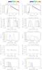 |
Fig. 2 Top to bottom: electron distribution function f(v); the spectral energy density of Langmuir waves W(k); in-source harmonic radio brightness temperature TT(k) (for k/kDe = 0.0225 to 0.0235, corresponding to ω/ωpe = 2 to 2.08); spectral energy density of ion-sound waves WS(k); in-source fundamental radio brightness temperature TT(k) (for k/kDe = 0. to 0.01, corresponding to ω/ωpe = 1 to 1.1) for a collisionally relaxing electron beam in homogeneous plasma (left column) and in inhomogeneous plasma with τD ≃ 0.24 s (right column). Each coloured line shows the distribution at a different time, as shown in the colour bar. |
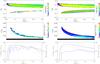 |
Fig. 3 Langmuir wave spectral energy density and radio emission in sfu over the first 0.4 s of beam evolution. Top: Langmuir wave spectral energy density W(k) normalised to the thermal level, against wavenumber k on the vertical axis, and time on the horizontal axis. Middle: the radio flux in sfu as a function of frequency, ν = ω/(2π), including the effects of absorption during propagation. The source size and plasma density profile are as described in the text, and the observed background flux from a thermal source of this size is ~10-2 sfu. Bottom: the total energy in Langmuir waves (solid line), backscattered Langmuir waves (negative wavenumber) only (dotted line), and radio emission (blue line), normalised by the thermal levels, against time. The left panel shows homogeneous plasma, the right, inhomogeneities with τD ≃ 2.4 s. |
The thermal Langmuir wave level is found by setting the LHS of Eq. (4) to zero and balancing the thermal (first and third) terms on the RHS, giving  (27)with λDe = 1/kDe = vTe/ωpe. The initial level of ion-sound waves is thermal (Kontar et al. 2012),
 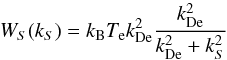 (28)and the initial EM brightness temperature is thermal, TT = Te.
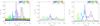 |
Fig. 5 Time profiles of the observed radio flux (the fundamental component at 1 GHz is not visible due to strong absorption between source and observer) for escape with coronal density scale height of H = 109 cm, in sfu including the quiet-Sun background in homogeneous plasma (no density fluctuations), averaged over frequency bands ν to ν + Δν for Δν = 1 MHz (left) and 5 MHz (middle) at ν as shown in the colour bar. The right panel shows Δν = 5 MHz for H = 6 × 108 cm. |
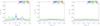 |
Fig. 6 Time profiles of the observed radio flux in sfu including the quiet-Sun background, averaged over frequency bands ν to ν + Δν for Δν = 5 MHz at ν as shown in the colour bar. Left to right, top to bottom: homogeneous plasma, and inhomogeneities with τD = 2.4 s and 0.24 s. |
3.2. Scattering by Ions
In plasma with equal ion and electron temperatures, Ti = Te = 1 MK, ion-sound waves are strongly damped, and ion-scattering dominates the Langmuir wave backscattering. We take an initial beam as given by Eq. (26) with a beam density of nb = 108 cm-3 ≃ 10-2ne. We note that this is for the initial power-law distribution. As collisional relaxation proceeds, a bump-on-tail distribution is produced, with a central velocity, density and width which vary over time due to continuing collisional losses. At this time, the majority of the beam electrons have thermalised, and so the level of Langmuir waves produced remains within the limits of weak-turbulence theory. In this section, we simulate electron-Langmuir wave evolution as given by Eqs. (3) and (4), and radio emission as in Eq. (14). We omit the terms involving ion-sound waves (Eqs. (9) and (16)) as the sound-wave damping rate is γS ≃ ωS, i.e the waves are damped over a timescale of less than one period, and the weak-turbulence equations will not accurately describe the behaviour (e.g. Melrose 1980b; Tsytovich 1995). Instead we consider the process of scattering by plasma-ions only.
Figure 2 shows, for the case of homogeneous plasma, the resulting electron distribution, the Langmuir and ion-sound wave spectral energy densities, normalised to  (see Eq. (27)), and the fundamental and harmonic radiation brightness temperatures. The fundamental emission reaches a brightness temperature of around TT ≃ 109 K, while the harmonic emission can reach TT ≃ 1011 K. These are the in-source brightness temperatures, whereas the observable brightness temperature will be reduced by a factor of exp( − τ), with τ the optical depth as in Eq. (24). As noted above this means fundamental emission at these levels will not be observable, and the harmonic component will be reduced by around an order of magnitude. The dispersion relation for electromagnetic waves is ω = (ωpe + c2k2)1/2 and so the wavenumber variation shown here will lead to emission at a small range of frequencies near ωpe and 2ωpe.
Langmuir wave scattering by plasma ions is described by Eq. (7). By taking the limit of vTi ≪ vTe in Eq. (7), we find the RHS is proportional to d/dk(kW(k)) (as in Mel’Nik & Kontar 2003), and we therefore require locally positive gradient, d/dk(kW(k)) > 0 for the backscattered waves to grow. Backscattering can then produce new regions of positive slope in the forwards wave spectrum, as seen in Fig. 2, and these each produce a peak in the backscattered spectrum, leading to the multiple peaked distribution seen at around 0.1 s, and the similar structure seen in the harmonic emission.
We now consider the effects of Langmuir wave diffusion in wavenumber due to density fluctuations, with coefficient D(k) given by Eq. (6). The parameters of small-scale density fluctuations are unknown in the low corona. However, previous work (Ratcliffe et al. 2012) has shown that the most important factor for Langmuir wave evolution is the diffusive time-scale τD, which we define here as  (29)where kb is the typical wavenumber of Langmuir waves in resonance with the reverse slope part of the electron distribution function. For a collisionally relaxing beam, this typical wavenumber varies over time, so we take the value at a time of 0.3s, kb ≃ 0.1kDe. We set the characteristic velocity to approximately the sound speed, v0 = 107 cm s-1, and consider τD ≃ 2.4 s, 0.24 s and 0.05 s. To relate this τD to the rms density fluctuation we must assume a value for q0, the characteristic wavenumber of fluctuations. For example, taking q0 = 6 × 10⁻⁴kDe corresponding to a length scale of 10 km, gives
  for τD ≃ 0.24 s. This may be compared with observations in the higher corona and solar wind, which show levels of the order
  to 10-2 (Cronyn 1972; Smith & Sime 1979).
Figure 2 also shows the electron, Langmuir wave and ion-sound wave distributions and the fundamental and harmonic radio brightness temperature for τD ≃ 0.24 s. Significant spreading of the Langmuir waves is evident, with a decrease in the backscattered wave level and consequently in the brightness of electromagnetic emission.
Figures 3 and 4 show the Langmuir wave spectral energy density and observable radio flux, calculated using Eq. (25), in sfu (Solar Flux Units, 1 sfu = 10-19 erg s-1 cm-2 Hz-1) for three cases of density fluctuations, with τD = 0.05,0.24,2.4 s as well as the homogeneous case. The small oscillations in radio wave energy seen between 0.2 and 0.4 s are a numerical effect probably due to the discrete wavenumber grid used in the simulation code. The calculated fluxes are a few to perhaps ten sfu while the duration of the simulated emission varies between approximately half a second for the homogeneous case down to around 0.1 s in the most inhomogeneous case. This duration is controlled by the Langmuir wave level, which in turn is controlled by the collisional relaxation of the electron beam.
Collisional relaxation also leads to the generation of Langmuir waves at smaller wavenumbers over time, which causes the emission to drift in frequency, in this case by approximately 50 MHz. Electromagnetic emission is more efficient at lower frequencies, and so the level of emission rises. This is seen clearly in the bottom panels of Figs. 3 and 4 where we plot the total energy in Langmuir waves, EL, backwards (negative wavenumber) Langmuir waves  and harmonic electromagnetic emission EH, all normalised to the thermal levels. Initially, the rise of the electromagnetic wave energy EH closely tracks the backscattered wave energy . However, for the two moderately inhomogeneous cases (top right and bottom left panels), we see the continued increase of electromagnetic wave energy after the backscattered Langmuir wave energy has peaked, between 0.15 to 0.3 s.
The observable thermal radio emission from our source, with size 0.2′ and temperature 106 K, including absorption, is approximately 10-2 sfu. In contrast, the average whole Sun radio emission at 2 GHz varies over the solar cycle between approximately 50 and 150 sfu, and so we take a reference value of 100 sfu at 2 GHz, scaling with frequency as in Benz (2009). In Fig. 5 we show the time profile of observed emission in homogeneous plasma including this background, averaged over frequency bands ν to ν + Δν. Figure 5 shows the result in homogeneous plasma for Δν = 1 MHz and 5 MHz and ν from 2.01 GHz to 2.05 GHz. The spiky nature of the emission in both time and frequency is evident. Figure 6 shows the fluxes for Δν = 5 MHz in homogeneous and inhomogeneous plasma. Inhomogeneity is seen to smooth out the time and frequency variations, as well as reducing the intensity of emission. The effects of absorption during propagation are illustrated in Fig. 5, where we show density scale heights of H = 109 cm and 6 × 108 cm, the latter giving a four-fold enhancement in the observed emission from the source.
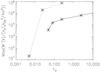 |
Fig. 7 Peak spectral energy density of backscattered Langmuir waves, W−(k), against the timescales τD for several values of plasma inhomogeneity. The solid line shows plasma with equal ion and electron temperatures, while the dashed line has Ti = 0.5Te. |
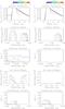 |
Fig. 8 Top to bottom: electron distribution function f(v); the spectral energy density of Langmuir waves W(k); in-source harmonic radio brightness temperature Tb(k); spectral energy density of ion-sound waves WS(k); in-source fundamental radio brightness temperature Tb(k) for a collisionally relaxing electron beam. Each coloured line shows the distribution at a different time, as shown in the colour bar. Left column: results in inhomogeneous plasma with τD ≃ 0.024 s, right column with τD ≃ 0.0024 s. |
3.3. Ion-sound wave scattering
For plasma with an electron temperature larger than the ion temperature, Te > Ti we can also consider the decay of Langmuir waves to an ion-sound wave, and a backscattered Langmuir wave, described by Eq. (9). We take Te = 106 K and Ti = 5 × 10⁵ K, with other parameters as in the previous section to obtain Fig. 8 which show the electron and wave distributions in inhomogeneous plasma with τD = 0.024 s and τD = 0.0024 s respectively. The level of backscattered Langmuir waves in these cases is far less affected by inhomogeneity than that due to ion-scattering alone, with complete suppression only for the shortest τD. The harmonic radio emission we see is of similar magnitudes to that seen in the previous section, but covers a slightly wider range in k-space, and therefore frequency, at a given time. The fundamental emission is again much weaker than the harmonic.
4. Discussion and conclusions
The numerical results presented in Figs. 2 and 8 show the tendency of plasma density inhomogeneities to suppress Langmuir wave backscattering. In Fig. 7 we plot the peak backwards Langmuir wave spectral energy density for several cases of density fluctuations, in both equal temperature plasma and plasma with Ti = 0.5Te. Both show a sharp decrease in backscattered level, but in the latter case this occurs only for much stronger inhomogeneity than the former. This is due to the relative efficiencies of the two backscattering processes, or equivalently their timescales. In general, the Langmuir wavenumber diffusion can suppress a process when τD is similar to the timescale of the process, as found in previous work (Ratcliffe et al. 2012) in relation to the interaction of Langmuir waves with beam electrons.
In the cases shown here, the inhomogeneity is too weak to significantly suppress the beam-plasma interaction, although we do see some slight electron acceleration, due to the transfer of energy from slower to faster electrons by the wavenumber diffusion. Comparing Fig. 8 with the homogeneous case in Fig. 2, the latter displays a broadened plateau in the electron distribution around 20vTe, where electrons have been accelerated. Stronger inhomogeneities, with τD ~ τql the quasilinear time for beam-plasma interaction, can lead to significant electron distribution tail self-acceleration. Here, we have seen that plasma emission from such a beam would be suppressed at GHz frequencies.
In-source brightness temperatures of 1011 K were seen in homogeneous plasma, corresponding to an observed flux of the order of a few sfu, potentially observable against the quiet Sun background. Even a low level of inhomogeneities can reduce these values by an order of magnitude, while strong fluctuations suppress the emission to the thermal level. The level of density fluctuations as commonly observed in the corona (Cronyn 1972; Smith & Sime 1979) with  km leads to suppression of electromagnetic emission for rms fluctuation magnitude of around
  for equal temperature plasma, and
  in plasma with larger electron than ion temperature. Therefore we expect no observable plasma emission at these levels of inhomogeneity in the emission source.
To conclude, we have developed an angle-averaged emission model for fundamental and harmonic plasma emission in collisional plasma, and presented simulation results from this in homogeneous plasma and plasma with weak density fluctuations. We find that the effects of density inhomogeneities on Langmuir wave backscattering can be very significant even for low levels of plasma inhomogeneity. This has important effects not only on the Langmuir wave evolution itself, but more significantly can suppress the production of plasma radio emission. For random density fluctuations with parameters as observed in the solar corona, Langmuir wavenumber diffusion can completely suppress plasma radio emission even in the presence of strong Langmuir wave turbulence. Moreover, these density fluctuations can simultaneously lead to electron self-acceleration, increasing the number of fast electrons yet decreasing or completely hiding the often-expected radio signature of Langmuir waves.
More precisely, ωL = kv with  the Langmuir wave frequency should be considered, but since k/kDe ≪ 1 for the excited Langmuir waves, ωL ≈ ωpe is good approximation (Vedenov 1963).
Acknowledgments
We thank the anonymous referee for the useful comments. This work was supported by an STFC STEP (Studentship Extension Programme) award (HR) and a STFC consolidated grant (EPK). Additionally, support by the Marie Curie PIRSES-GA-2011-295272 RadioSun project, the European Research Council under the SeismoSun Research Project No. 321141 is gratefully acknowledged.
References
- Benz, A. O. 2009, in Landolt-Börnstein − Group VI Astronomy and Astrophysics, Vol. 4B, Solar System, ed. J. Trümper (Berlin: Springer Heidelberg), 103 [Google Scholar]
- Cairns, I. H. 2000, Phys. Plasmas, 7, 4901 [NASA ADS] [CrossRef] [Google Scholar]
- Cronyn, W. M. 1972, ApJ, 171, L101 [NASA ADS] [CrossRef] [Google Scholar]
- Dennis, B. R. 1985, Sol. Phys., 100, 465 [NASA ADS] [CrossRef] [Google Scholar]
- Drummond, W., & Pines, D. 1964, Ann. Phys. (NY), 28, 478 [NASA ADS] [CrossRef] [Google Scholar]
- Emslie, A. G., & Smith, D. F. 1984, ApJ, 279, 882 [NASA ADS] [CrossRef] [Google Scholar]
- Ginzburg, V. L., & Zhelezniakov, V. V. 1958, Sov. Astron., 2, 653 [Google Scholar]
- Gurnett, D. A., Marsch, E., Pilipp, W., Schwenn, R., & Rosenbauer, H. 1979, J. Geophys. Res., 84, 2029 [NASA ADS] [CrossRef] [Google Scholar]
- Hamilton, R. J., & Petrosian, V. 1987, ApJ, 321, 721 [NASA ADS] [CrossRef] [Google Scholar]
- Jeffrey, N. L. S., & Kontar, E. P. 2013, ApJ, 766, 75 [NASA ADS] [CrossRef] [Google Scholar]
- Karlicky, M. 1998, Sol. Phys., 179, 421 [NASA ADS] [CrossRef] [Google Scholar]
- Karlický, M., & Kontar, E. P. 2012, A&A, 544, A148 [NASA ADS] [CrossRef] [EDP Sciences] [Google Scholar]
- Kontar, E. P., & Pécseli, H. L. 2002, Phys. Rev. E, 65, 066408 [NASA ADS] [CrossRef] [Google Scholar]
- Kontar, E. P., Ratcliffe, H., & Bian, N. H. 2012, A&A, 539, A43 [NASA ADS] [CrossRef] [EDP Sciences] [Google Scholar]
- Li, B., Cairns, I. H., & Robinson, P. A. 2008, J. Geophys. Res. (Space Physics), 113, 6104 [Google Scholar]
- Lifshitz, E. M., & Pitaevskii, L. P. 1981, Physical Kinetics (Butterworth Heinemann) [Google Scholar]
- Mel’Nik, V. N., & Kontar, E. P. 2003, Sol. Phys., 215, 335 [NASA ADS] [CrossRef] [Google Scholar]
- Melrose, D. B. 1980a, Plasma astrophysics: Nonthermal processes in diffuse magnetized plasmas, Astrophysical Applications, 2 [Google Scholar]
- Melrose, D. B. 1980b, Plasma Astrophysics, Volumes 1 and 2 [Google Scholar]
- Melrose, D. B., & Stenhouse, J. E. 1979, A&A, 73, 151 [NASA ADS] [Google Scholar]
- Muschietti, L., Goldman, M. V., & Newman, D. 1985, Sol. Phys., 96, 181 [NASA ADS] [CrossRef] [Google Scholar]
- Newbury, J. A., Russell, C. T., Phillips, J. L., & Gary, S. P. 1998, J. Geophys. Res., 103, 9553 [Google Scholar]
- Nishikawa, K., & Ryutov, D. D. 1976, J. Phys. Soc. Japan, 41, 1757 [NASA ADS] [CrossRef] [Google Scholar]
- Ratcliffe, H., Bian, N. H., & Kontar, E. P. 2012, ApJ, 761, 176 [NASA ADS] [CrossRef] [Google Scholar]
- Smith, D. F., & Sime, D. 1979, ApJ, 233, 998 [NASA ADS] [CrossRef] [Google Scholar]
- Sturrock, P. A. 1964, NASA Spec. Publ., 50, 357 [Google Scholar]
- Tsiklauri, D. 2011, Phys. Plasmas, 18, 052903 [NASA ADS] [CrossRef] [Google Scholar]
- Tsytovich, V. N. 1970, Nonlinear Effects in Plasma (Springer) [Google Scholar]
- Tsytovich, V. N. 1995, Lectures on Non-linear Plasma Kinetics, eds. V. N. Tsytovich, & D. ter Haar [Google Scholar]
- Vedenov, A., Velikhov, E., & Sagdeev, R. 1962, Quasi-linear theory of plasma oscillations, Tech. Rep., Kurchatov Inst. of Atomic Energy, Moscow [Google Scholar]
- Vedenov, A. A. 1963, J. Nucl. Energy, 5, 169 [NASA ADS] [CrossRef] [Google Scholar]
- Zheleznyakov, V. V., & Zaitsev, V. V. 1970, Sov. Astron, 14, 47 [Google Scholar]
All Figures
|
Fig. 1 Geometry of a model coronal loop. Within the loop the plasma density is approximately ne, with superimposed weak random density fluctuations. A fast electron population is produced in the source region, shaded dark grey, which relaxes collisionally, producing Langmuir waves and thus radio emission. Radio emission arises from the source region of linear size d ≃ 109 cm measured perpendicular to the loop axis, of the order of the typical cross-sectional size of a coronal loop. An observer at 1 AU sees a source with angular radius θ. The surrounding plasma has an exponential density profile of scale height H. |
| In the text | |
|
Fig. 2 Top to bottom: electron distribution function f(v); the spectral energy density of Langmuir waves W(k); in-source harmonic radio brightness temperature TT(k) (for k/kDe = 0.0225 to 0.0235, corresponding to ω/ωpe = 2 to 2.08); spectral energy density of ion-sound waves WS(k); in-source fundamental radio brightness temperature TT(k) (for k/kDe = 0. to 0.01, corresponding to ω/ωpe = 1 to 1.1) for a collisionally relaxing electron beam in homogeneous plasma (left column) and in inhomogeneous plasma with τD ≃ 0.24 s (right column). Each coloured line shows the distribution at a different time, as shown in the colour bar. |
| In the text | |
|
Fig. 3 Langmuir wave spectral energy density and radio emission in sfu over the first 0.4 s of beam evolution. Top: Langmuir wave spectral energy density W(k) normalised to the thermal level, against wavenumber k on the vertical axis, and time on the horizontal axis. Middle: the radio flux in sfu as a function of frequency, ν = ω/(2π), including the effects of absorption during propagation. The source size and plasma density profile are as described in the text, and the observed background flux from a thermal source of this size is ~10-2 sfu. Bottom: the total energy in Langmuir waves (solid line), backscattered Langmuir waves (negative wavenumber) only (dotted line), and radio emission (blue line), normalised by the thermal levels, against time. The left panel shows homogeneous plasma, the right, inhomogeneities with τD ≃ 2.4 s. |
| In the text | |
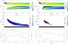 |
Fig. 4 As Fig. 3 for inhomogeneous plasma with τD = 0.24 s (left) and 0.05 s (right) respectively. |
| In the text | |
|
Fig. 5 Time profiles of the observed radio flux (the fundamental component at 1 GHz is not visible due to strong absorption between source and observer) for escape with coronal density scale height of H = 109 cm, in sfu including the quiet-Sun background in homogeneous plasma (no density fluctuations), averaged over frequency bands ν to ν + Δν for Δν = 1 MHz (left) and 5 MHz (middle) at ν as shown in the colour bar. The right panel shows Δν = 5 MHz for H = 6 × 108 cm. |
| In the text | |
|
Fig. 6 Time profiles of the observed radio flux in sfu including the quiet-Sun background, averaged over frequency bands ν to ν + Δν for Δν = 5 MHz at ν as shown in the colour bar. Left to right, top to bottom: homogeneous plasma, and inhomogeneities with τD = 2.4 s and 0.24 s. |
| In the text | |
|
Fig. 7 Peak spectral energy density of backscattered Langmuir waves, W−(k), against the timescales τD for several values of plasma inhomogeneity. The solid line shows plasma with equal ion and electron temperatures, while the dashed line has Ti = 0.5Te. |
| In the text | |
|
Fig. 8 Top to bottom: electron distribution function f(v); the spectral energy density of Langmuir waves W(k); in-source harmonic radio brightness temperature Tb(k); spectral energy density of ion-sound waves WS(k); in-source fundamental radio brightness temperature Tb(k) for a collisionally relaxing electron beam. Each coloured line shows the distribution at a different time, as shown in the colour bar. Left column: results in inhomogeneous plasma with τD ≃ 0.024 s, right column with τD ≃ 0.0024 s. |
| In the text | |
Current usage metrics show cumulative count of Article Views (full-text article views including HTML views, PDF and ePub downloads, according to the available data) and Abstracts Views on Vision4Press platform.
Data correspond to usage on the plateform after 2015. The current usage metrics is available 48-96 hours after online publication and is updated daily on week days.
Initial download of the metrics may take a while.