| Issue |
A&A
Volume 561, January 2014
|
|
|---|---|---|
| Article Number | L4 | |
| Number of page(s) | 5 | |
| Section | Letters | |
| DOI | https://doi.org/10.1051/0004-6361/201322975 | |
| Published online | 23 December 2013 | |
Possible astrometric discovery of a substellar companion to the closest binary brown dwarf system WISE J104915.57–531906.1⋆,⋆⋆
1
ESO, Av. Alonso de Cordova 3107, 19001 Casilla,
Santiago 19,
Chile
e-mail:
This email address is being protected from spambots. You need JavaScript enabled to view it.
2
Institut d’Astronomie et d’Astrophysique, Université Libre de
Bruxelles (ULB), 1050
Bruxelles,
Belgium
3
Departamento de Física y Astronomía, Universidad de
Valparaiso, Av. Gran Bretaña 1111,
5030 Playa Ancha, Casilla, Chile
4
Las Campanas Observatory, Carnegie Institution of Washington,
Colina el Pino, 601
Casilla, La Serena,
Chile
5
ESO, Karl-Schwarzschild-str. 2, 85478
Garching,
Germany
Received:
3
November
2013
Accepted:
4
December
2013
Abstract
Using FORS2 on the Very Large Telescope, we have astrometrically monitored over a period of two months the two components of the brown dwarf system WISE J104915.57-531906.1, the closest one to the Sun. Our astrometric measurements – with a relative precision at the milli-arcsecond scale – allowed us to detect the orbital motion and derive more precisely the parallax of the system, leading to a distance of 2.020 ± 0.019 pc. The relative orbital motion of the two objects is found to be perturbed, which leads us to suspect the presence of a substellar companion around one of the two components. We also performed VRIz photometry of the two components and compared this with models. We confirm the flux reversal of the T dwarf.
Key words: binaries: visual / parallaxes / astrometry / brown dwarfs
Based on data obtained with the ESO Very Large Telescope under programme 291.C-5004.
Figures 2 and 3 and Table 3 are available in electronic form at http://www.aanda.org
Senior Research Associate, F.R.S.-FNRS, Belgium.
© ESO, 2013
1. Introduction
Very recently, Luhman (2013) identified WISE J104915.57–531906.1 (hereafter Luhman 16AB, to follow the nomenclature of Burgasser et al. 2013a), a very red binary star with an incredibly high proper motion of ∼3″/yr and a distance of ∼2 pc, making it the third-closest system to the Sun, after α Cen and Barnard’s star. The two objects in Luhman 16AB are separated by 1.5′′, with the primary being a brown dwarf (BD) of spectral type L8.
In Kniazev et al. (2013), we reported comprehensive follow-up observations of this newly detected system, confirming the spectral types of the two BDs (L8 ± 1, T1 ± 2) and, based on the low relative radial velocity of the two components, confirmed that they form a gravitationally bound system. Our JHKS photometry yields colours consistent with the spectroscopically derived spectral types, while a comparison of the apparent magnitudes with models leads to a distance of ∼2.25 pc, in agreement with the parallax of Luhman (2013). The available kinematic and photometric information excludes the possibility that the object may belong to any of the known nearby young moving groups or associations. For the given spectral types and absolute magnitudes, 1 Gyr theoretical models – DUSTY (Baraffe et al. 2002) and BT-Settl (Allard et al. 2011) – predict masses of 0.04–0.05 M⊙ for the primary, and 0.03–0.05 M⊙ for the secondary. The objects remain in the substellar regime even if they are 10 Gyr old.
Gillon et al. (2013, see also Biller et al. 2013) reported complex quasi-periodic (4.87 h) near-infrared photometric variability at ∼0.1 mag level, which they associated with the rotation of the secondary. They did not detect a transit during their 12-night monitoring. Burgasser eta al. (2013b) also reported resolved near-infrared spectroscopy and photometry of Luhman 16AB, which revealed strong H2O and CO absorption features in the spectra of the two components, the secondary also showing weak CH4 absorption. They found the system to exhibit a “flux reversal”, that is, the T dwarf secondary appears brighter in the 0.9–1.3 μm wavelength range, but is fainter at shorter wavelengths.
In this paper, we present additional imaging observations of the individual components of Luhman 16AB, with the aim to start a long-term astrometric campaign, to obtain a more definitive parallax and the orbit of the system. Based on GMOS observations and additional archival data from DSS, DENIS, and 2MASS, Luhman (2013) found a set of six positions over 23 years, yielding a parallax (ϖ) of 496 ± 37 mas. He also obtained − 2759 ± 6 and 354 ± 6 mas yr-1 for the proper motion μα ∗ (=μαcosδ) and μδ. In a note on astro-ph, Mamajek (2013) compiled some previously found positions from the ESO Schmidt red and GSC 2.3 catalogues. Using these additional points, we obtain a revised parallax of ϖ = 514 ± 26 mas.
2. Observations and data reduction
Over a period of two months starting in mid-April 2013, Luhman 16AB was observed with the FORS2 multi-purpose optical instrument (Appenzeller et al. 1998) attached to Unit 1 of the Very Large Telescope. The high-resolution collimator was used with 2 × 2 binning, resulting in a pixel scale of 0.125′′ and a field of view of 4.1′. The MIT CCD was used, which is comprised of two chips, separated by a gap of 10.8′′. Luhman 16AB lies in the upper chip (CHIP1), and in this study we have only used stars on this chip to avoid introducing the additional misalignment between the two chips.
Observations were made using the I-band filter (I_BESS+77) on 12 epochs over the period from 14 April to 22 June 2013, with each epoch generally separated by 5 or 6 days. For each epoch, at least 21 images were taken (although not all were used, see below). The exposure time ranged from 15 to 60 s, and the seeing was always better than 1.2′′, ensuring that the two components of the binary system were always well separated. Observations were only made when the object was at airmass below ∼1.2. A detailed log of the observations is provided in Table 3, while a typical image is shown in Fig. 2.
The individual images of a single night were stacked by minimising the scatter in Δα∗ = Δαcosδ and Δδ for every source, where as usual, α and δ are the right ascension and the declination. The sample of images was limited to those where the two components of Luhman 16AB were resolved and measured. In each night, a reference image was adopted and the median of the shift derived for all sources but Luhman 16AB was determined. The resulting uncertainty on the positions, between 2 and 10 mas (see the values σα ∗ and σδ in Table 3), was computed as the standard deviation of the 5th–95th percentiles of the stacked positions. The same procedure was then applied to every night relative to the first one. The ICRS coordinates were finally restored by measuring the position of one star in one of these images.
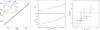 |
Fig. 1 Left: old and new observations adjusted. The dotted line represents the solution based upon Luhman (2013) and Mamajek (2013). The black continuous line represents the motion of the barycentre from our solution. The inset zooms onto the region covered by the FORS2 observations. The red (resp. blue) line represents the motion of the L (resp. T) dwarf. Middle: relative positions obtained with FORS2 during our two-month monitoring campaign and the best parabolic fits. Right: residuals of the FORS2 data based on the parabolic fit. |
The accuracy of this stacking procedure relies heavily upon a key assumption: no other point source on the field of view is moving during the two-month observation campaign. Point source here means a single star with a noticeable parallax and/or proper motion or a binary (unresolved or with only one component visible) with a significant orbital motion. At the 5 mas level, no disturbing point source is present in the field of view, thus making the stacked image very reliable.
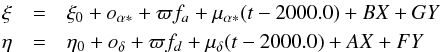
In addition to our astrometric monitoring in the I band, on 16 June 2013 we have also obtained, images of Luhman 16AB with FORS2 in the V, R, and z bands with the v_HIGH, R_SPECIAL and z_GUNN filters and exposure times of 480, 120, and 5 s, respectively. The resulting images are also shown in Fig. 2.
3. Astrometric models
Two sets of observations are available: the absolute positions of the photocentre over 23 years from archival data and the absolute positions of the two components over our two month monitoring. Even though the latter are much more precise, a campaign of two months is too short to derive either the parallax or the proper motion. They can nevertheless be combined with the previously published data to improve the precision of the fundamental astrometric parameters that constrain the size and orientation of the orbit. On the other hand, the positions of the two components can be changed into relative positions of one component with respect to the other, thus removing the effect of the parallax and proper motion and keeping only the orbital parameters.
3.1. Two-body orbital model
The motion of a resolved binary is fully described by the motion of its barycentre (position, parallax, and proper motion) and the orbital motion of each component around it (Binnendijk 1960). The two orbits only differ by their size and the argument of the periastron, 180° apart. Thirteen parameters are thus required. However, a careful selection of these parameters can make the fitting procedure much more straightforward. Adopting the Thiele-Innes parameters for instance for the primary makes nine parameters appear linearly, instead of only five with the Campbell orbital elements (e.g. Pourbaix & Boffin 2003). With the orbit of the primary setting up the unit, the orbit of the secondary is just its scaled image, the scaling factor (ρ) lying between 0 and + ∞. In practice, a grid search was used for the remaining four nonlinear parameters.
Even though every step leading to the stacked image was performed very thoroughly, the
transformation of the relative positions into the absolute ones relies upon only one
direct measurement, thus making it the single point of failure. To restore some
reliability, two linear parameters (oα ∗ and
oδ) were therefore added to cope with some
misalignment between the old and new dataset. The resulting model is therefore given by
 for
the primary,
for
the primary, 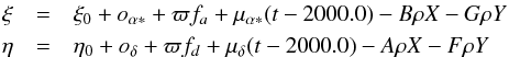 for
the secondary, and
for
the secondary, and  for
the barycentre. fa and
fd denote the parallactic factors (Kovalevsky & Seidelmann 2004),
ξ = αcosδ, and
η = δ. Luhman
(2013) assumed that on the old plates, the measured photocentre matches the epoch
barycentre. As the exact orbit is not available yet, one cannot say how incorrect this
assumption is. During our observation campaign, the offset of the photocentre with respect
to the barycentre ranged from 40 mas in I to 100 mas in
V. The resulting least-squares fit (with a grid for the few nonlinear
parameters) is illustrated in Fig. 1.
for
the barycentre. fa and
fd denote the parallactic factors (Kovalevsky & Seidelmann 2004),
ξ = αcosδ, and
η = δ. Luhman
(2013) assumed that on the old plates, the measured photocentre matches the epoch
barycentre. As the exact orbit is not available yet, one cannot say how incorrect this
assumption is. During our observation campaign, the offset of the photocentre with respect
to the barycentre ranged from 40 mas in I to 100 mas in
V. The resulting least-squares fit (with a grid for the few nonlinear
parameters) is illustrated in Fig. 1.
3.2. Quadratic approximation
Even though two components exhibit a relative motion that prevents them from being fully described by two single-star solutions (sharing a common parallax and proper motion), this relative motion is so small that using the full orbital model from the previous section to describe it is simply overkill because it offers too much freedom with respect to the number of data points available to constrain the parameters of the models. For a long enough orbital period, over an observation campaign of two months, both Δξ and Δη can be modelled with an arc of parabola without biasing the conclusion with respect to the true orbital Keplerian model. Over the full orbital model, this quadratic model also offers the advantage of being linear, thus yielding a straightforward unique least-squares solution.
The validity of this simplification was assessed through a large-scale Monte-Carlo simulation. Five million orbits were generated (random orientation, period normally distributed around 20 years). For all of them, we derived twelve positions for the same dates as the actual observations and added a probable noise. At the 3σ-level, no quadratic fit was distinguishable from the genuine orbital one.
3.3. Results
The results of the least-squares fit of the absolute positions (i.e. model from Sect. 3.1) from Luhman (2013), Mamajek (2013) and FORS2 are given in Table 1 and are plotted in Fig. 1a. The contribution of the primary to the χ2 is 20% higher than that of the secondary, thus suggesting that a companion might be present around the former and cause it to oscillate.
Astrometric results based on the old and new absolute positions and those obtained by Luhman (2013).
The parabolic least-squares fit of the relative positions is more difficult to assess. Both Δα ∗ and Δδ were fitted with distinct parabolae (Fig. 1b). The higher χ2 was then used to derive the probability of rejecting the parabola (i.e. a two-body model) by accident even though it holds. Whereas for a single parabola this probability is tabulated and directly available, we relied upon extensive Monte-Carlo simulations to quantify the effect of taking the higher of the two χ2 instead of just one. The probability of rejecting the parabola by accident is 12.95%. This sole value is too high to draw any definitive conclusion.
On the other hand, the residuals of the parabolic fit are highly correlated (Pearson’s r = 0.95; Fig. 1c). In our Monte-Carlo simulation of genuine binaries, such a high correlation between the residuals is obtained for only 0.002% of the systems. There is therefore a strong indication to reject the basic two-body model.
4. Photometry of the components
Using our FORS2 observations, we also estimated the magnitudes of the two components of Luhman 16AB in the V, R, I, and z bands (Table 2). Point-spread-function photometry was performed with DAOPHOT, using the FORS2 standards E5 and LTT4816. They clearly confirm the flux reversal mentioned by Burgasser et al. (2013a) because the T dwarf becomes the brightest of the two in the z-band.
Apparent magnitudes of the components of Luhman 16AB.
A comparison between our photometry and the most recent models from the Lyon group (BT-Settl; Allard et al. 2011) is shown in Fig. 3, where we used the effective temperatures as derived by Kniazev et al. (2013). To convert the results to absolute magnitudes we used the distance of 2.02 ± 0.02 pc established in this work, while the error bars reflect uncertainties in effective temperatures, distance modulus, and photometry. The model isochrones are plotted for 0.1, 1.0, and 5 Gyr1. Owing to their intrinsic faintness in the optical, late-L and T dwarfs have mostly been studied in the near-infrared. Consequently, there are very few works available for a comprehensive comparison of the optical photometry with models, and with our photometry as well. Dahn et al. (2002) published optical VRI photometry and colours for 28 ultracool dwarfs with distances known from parallax measurements. Their sample contains 17 L dwarfs and three T dwarfs, but only five of them have spectral type L8 or later. The resulting absolute I-band magnitude, MI, from their work is ∼19 for L8, and ∼19.5 for T2, while in the R band it is ∼21.7, in agreement with our results for Luhman 16AB. Dobbie et al. (2002) also found MI ∼ 19 for the spectral type L8. The age of Luhman 16AB has been constrained to be less than about 4.5 Gyr based on the presence of the lithium line, while from the absence of low surface gravity indicators in the spectra, it is clear that the system is not young (Burgasser et al. 2013a,b). We therefore expect the 1.5 Gyr isochrones to be the most suitable for comparison. The model isochrones seem to overestimate the flux at the L/T transition in RIz, and somewhat underestimate it in the V band.
5. Discussion
The FORS2 data, once combined with the data of Luhman (2013) and Mamajek (2013), yield a significant improvement of the precision of the parallax derived by Luhman (2013). Yet, the FORS2 positions alone indicate that a two-body system is very unlikely, whereas an additional companion would explain the observed wobbles. Such a companion must have a mass lower than the brown dwarfs in the system, because i) it would otherwise have been seen in direct imaging or spectroscopy; and ii) a system with two equal-mass brown dwarfs would not be detected because there would be no motion of the photocentre. A 10 MJup object in orbit of the primary component of Luhman 16AB, which for simplicity we will assume has a mass of 0.05 M⊙, will have a maximum separation on sky of 0.06 to 0.19 arcsec, for an orbital period between two months and one year, respectively. If we assume that this companion has a negligible luminosity compared with that of Luhman 16A, it will induce an astrometric signal between 10 and 32 mas, depending on the orbital period. One might expect that a more massive companion would lead to a stronger astrometric signal, but this is not necessarily the case, because this companion would now contribute light to the combined system, and although the barycentre may change more, the photocentre – which is what we detect – would not. Assuming that the luminosity of a BD scales as the square of its mass (e.g. Burrows & Liebert 1993), we find that a 20 MJup induces a change of the barycentre of between 20 and 60 mas, but a change of the photocentre of between 10 and 30 mas. A more massive companion would lead to even weaker motions of the photocentre. On the other hand, a much smaller companion of for example 3 MJup, would lead to a maximum motion of 10 mas for a period of one year. Although it is still too early to be able to characterise the possible companion, it seems likely that it has a mass between a few and ∼30 Jupiter masses, but the latter could then be discovered by adaptive optics, given the expected separation on the sky. At the least, the above discussion shows that the presence of such a companion is compatible with our astrometric signal.
If this companion would have a planetary mass (below the deuterium-burning limit), this would be the first exoplanet around a brown dwarf discovered by astrometry, and possibly the closest exoplanet to the Sun (given that the one about α Cen B is still debated; Hatzes 2013). Until now, only eight planets are known around brown dwarfs2 and they were found via microlensing and direct imaging. Microlensing allows finding a close-in population of planets (0.2–0.9 AU; see, for a summary, Han et al. 2013). These are likely to have formed in a protoplanetary disc. They do show a higher planet-to-host mass ratio than the imaging-discovered planets but nothing is known about the physical nature of these planetary mass companions because of the large distances of these systems, which prevent follow-up studies. In contrast, the imaging method finds only massive planetary-mass companions at large distance (tens or even several hundreds of AU) from their host star. These systems more closely resemble binary substellar systems than planetary systems because the planetary mass companions could not have formed from a proto-planetary disc but rather during the collapse and fragmentation of a proto-stellar/proto-BD molecular cloud (Jayawardhana & Ivanov 2006). If this tells us
that planets do form around brown dwarfs, the short-period range is still unexplored, and Luhman 16AB provides us with a unique opportunity to probe it. We also note that planets inside binary systems are not unheard of and, for example, Roell et al. (2012) identified 57 exoplanet host stars with stellar companions. In the past years, imaging campaigns found stellar companions around several dozen exoplanet host stars that were formerly believed to be single stars (see e.g. Raghavan et al. 2006; Mugrauer & Neuhäuser 2009). Most of these exoplanet candidates are in an S-type orbit configuration, with the exoplanet surrounding one stellar component of the binary. As is well known, multiple systems are stable only if they are hierarchical, with period ratios exceeding 10 (see e.g. Cuntz 2013, and references therein). Because the companion we tentatively detected probably has a period of only a few months (because otherwise we would not have been able to detect it in our two-month monitoring), while the orbital period of Luhman 16AB is of the order of 25 years Kniazev et al. (2013), this is certainly the case here. Finally, we note that if one of the two brown dwarfs in Luhman 16AB has indeed a substellar companion in close orbit, it will probably lead to a radial velocity change of the order of 3–5 km s-1. This assumes that the companion’s orbit around the brown dwarf is seen edge-on. As our astrometric measurements seem to tentatively indicate that components A and B of Luhman 16AB are in an almost edge-on orbit, this seems a reasonable assumption for the orbit of the third component. We therefore encourage high-precision radial velocity monitoring of the system on short time-scales.
Online material
Observation log book.
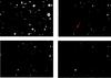 |
Fig. 2 FORS2 observations of Luhman 16AB in various bands: V (top left), R (top right), I (bottom left) and z (bottom right). The two components are indicated in the R-band image with an arrow. It is clear from these images that the two components are very red objects. Each image is a very small subset of the full field of view of FORS2, showing only 1.62 × 1.15 arcmin. North is up and east is to the left. |
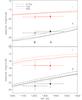 |
Fig. 3 Comparisons between observations and models. Circles show the absolute photometry of the system (filled symbols for the primary and open for the secondary), while model isochrones are plotted for 0.1, 1.0, and 5 Gyr. |
Isochrones in Johnson VRI available at http://phoenix.ens-lyon.fr/Grids/BT-Settl/. For the nonstandard filter z, we convolved the model spectra with the filter transmission curve, and converted this to magnitudes by assuming zVega = 0.
Acknowledgments
It is a pleasure to thank Petro Lazorenko for useful discussions, as well as an anonymous referee for comments that improved the paper. R.K. acknowledges support from FONDECYT through grants No. 1130140.
References
- Allard, F., Homeier, D., & Freytag, B. 2011, 16th Cambridge Workshop on Cool Stars, Stellar Systems, and the Sun, eds. M. J.-K. Christopher, K. B. Mathew, & A. W. Andrew, ASP Conf. Ser., 448, 91 [Google Scholar]
- Appenzeller, I.,Fricke, K.,Fürtig, W., et al. 1998, The Messenger, 94, 1 [NASA ADS] [Google Scholar]
- Baraffe, I.,Chabrier, G.,Allard, F., &Hauschildt, P. H. 2002, A&A, 382, 563 [NASA ADS] [CrossRef] [EDP Sciences] [Google Scholar]
- Biller, B. A.,Crossfield, I. J. M.,Mancini, L., et al. 2013, ApJ, 778, 10 [Google Scholar]
- Binnendijk, L. 1960, Properties of Double Stars (University of Pennsylvania Press) [Google Scholar]
- Burgasser, A. J., Faherty, J., Beletsky, Y., et al. 2013a, Mem. Soc. Astron. It., submitted [arXiv:1307.6916] [Google Scholar]
- Burgasser, A. J.,Sheppard, S. S., &Luhman, K. L. 2013b, ApJ, 772, 129 [NASA ADS] [CrossRef] [Google Scholar]
- Burrows, A., &Liebert, J. 1993, Rev. Mod. Phys., 65, 301 [NASA ADS] [CrossRef] [Google Scholar]
- Cuntz, M. 2013, ApJ, 780, 14 [Google Scholar]
- Dahn, C. C.,Harris, H. C.,Vrba, F. J., et al. 2002, AJ, 124, 1170 [NASA ADS] [CrossRef] [Google Scholar]
- Dobbie, P. D.,Kenyon, F.,Jameson, R. F., &Hodgkin, S. T. 2002, MNRAS, 331, 445 [NASA ADS] [CrossRef] [Google Scholar]
- Gillon, M.,Triaud, A. H. M. J.,Jehin, E., et al. 2013, A&A, 555, L5 [NASA ADS] [CrossRef] [EDP Sciences] [Google Scholar]
- Han, C.,Jung, Y. K.,Udalski, A., et al. 2013, ApJ, 778, 38 [NASA ADS] [CrossRef] [Google Scholar]
- Hatzes, A. 2013, ApJ, 770, 133 [NASA ADS] [CrossRef] [Google Scholar]
- Jayawardhana, R., &Ivanov, V. D. 2006, Science, 313, 1279 [NASA ADS] [CrossRef] [PubMed] [Google Scholar]
- Kniazev, A. Y.,Vaisanen, P.,Mužić, K., et al. 2013, ApJ, 770, 124 [NASA ADS] [CrossRef] [Google Scholar]
- Kovalevsky, J., & Seidelmann, P. K., 2004, Fundamentals of Astrometry (Cambridge University Press) [Google Scholar]
- Luhman, K. L. 2013, ApJ, 767, L1 [NASA ADS] [CrossRef] [Google Scholar]
- Mamajek, E. E. 2013 [arXiv:1303.5345] [Google Scholar]
- Mugrauer, M., &Neuhäuser, R. 2009, A&A, 494, 373 [NASA ADS] [CrossRef] [EDP Sciences] [Google Scholar]
- Pourbaix, D., &Boffin, H. M. J. 2003, A&A, 398, 1163 [NASA ADS] [CrossRef] [EDP Sciences] [Google Scholar]
- Raghavan, D.,Henry, T. J.,Mason, B. D., et al. 2006, ApJ, 646, 523 [NASA ADS] [CrossRef] [MathSciNet] [Google Scholar]
- Roell, T.,Neuhäuser, R.,Seifahrt, A., &Mugrauer, M. 2012, A&A, 542, A92 [NASA ADS] [CrossRef] [EDP Sciences] [Google Scholar]
All Tables
Astrometric results based on the old and new absolute positions and those obtained by Luhman (2013).
All Figures
|
Fig. 1 Left: old and new observations adjusted. The dotted line represents the solution based upon Luhman (2013) and Mamajek (2013). The black continuous line represents the motion of the barycentre from our solution. The inset zooms onto the region covered by the FORS2 observations. The red (resp. blue) line represents the motion of the L (resp. T) dwarf. Middle: relative positions obtained with FORS2 during our two-month monitoring campaign and the best parabolic fits. Right: residuals of the FORS2 data based on the parabolic fit. |
| In the text | |
|
Fig. 2 FORS2 observations of Luhman 16AB in various bands: V (top left), R (top right), I (bottom left) and z (bottom right). The two components are indicated in the R-band image with an arrow. It is clear from these images that the two components are very red objects. Each image is a very small subset of the full field of view of FORS2, showing only 1.62 × 1.15 arcmin. North is up and east is to the left. |
| In the text | |
|
Fig. 3 Comparisons between observations and models. Circles show the absolute photometry of the system (filled symbols for the primary and open for the secondary), while model isochrones are plotted for 0.1, 1.0, and 5 Gyr. |
| In the text | |
Current usage metrics show cumulative count of Article Views (full-text article views including HTML views, PDF and ePub downloads, according to the available data) and Abstracts Views on Vision4Press platform.
Data correspond to usage on the plateform after 2015. The current usage metrics is available 48-96 hours after online publication and is updated daily on week days.
Initial download of the metrics may take a while.