| Issue |
A&A
Volume 561, January 2014
|
|
|---|---|---|
| Article Number | A135 | |
| Number of page(s) | 13 | |
| Section | Atomic, molecular, and nuclear data | |
| DOI | https://doi.org/10.1051/0004-6361/201322866 | |
| Published online | 23 January 2014 | |
Stark broadening of lines from transition between states n = 3 to n = 2 in neutral helium
An experimental and computer-simulation study ⋆
1 Departamento de Óptica, Universidad de Valladolid, 47071 Valladolid, Spain
e-mail: This email address is being protected from spambots. You need JavaScript enabled to view it.
2 University of Novi Sad, Faculty of Sciences, Department of Physics, Trg Dositeja Obradovića 4, 21000 Novi Sad, Serbia
e-mail: This email address is being protected from spambots. You need JavaScript enabled to view it.
Received: 17 October 2013
Accepted: 3 December 2013
Abstract
Context. The Stark broadening of the spectral lines of the wavelengths 501.6, 667.8, 728.1, 388.9, 587.6, and 706.5 nm from neutral helium in plasmas are studied theoretically and experimentally.
Aims. The aim of this work is to provide information about the connection between the shape and width of spectral lines and the electron density and temperature to be used as a diagnostic tool.
Methods. The theoretical calculations were carried out through molecular dynamics computer simulations with noninteracting particles. The experimental measurements were done in a plasma of pure helium generated in an electromagnetically driven T-tube. The plasma diagnostics used previous results about the Stark broadening of the He I 447.1 nm and He I 492.2 nm lines and the coherence between the shape of these spectra and those obtained here. The electron temperature was obtained through a Boltzmann-plot of eight lines of Si II.
Results. Several tables of width and shift are provided in a wide range of electron density and temperature. Furthermore, we supply several fitting formulas, which allow calculating the plasma electron density from the measured values of the spectral line widths. The results obtained in the laboratory and in the simulations are compared with the data from the literature.
Key words: line: profiles / plasmas / techniques: spectroscopic / methods: numerical / methods: laboratory: atomic / instrumentation: spectrographs
Tables of FWHM and shifts are only available at the CDS via anonymous ftp to cdsarc.u-strasbg.fr (130.79.128.5) or via http://cdsarc.u-strasbg.fr/viz-bin/qcat?J/A+A/561/A135
© ESO, 2014
1. Introduction
The Stark broadening of the helium lines from the transitions between the states with principal quantum number n = 2 and n = 3 were studied. These are transitions in the optical range, with wavelengths of 501.6, 667.8, 728.1, 388.9, 587.6, and 706.5 nm (which we refer to as He I 5016, 6678, 7281, 3889, 5876, and 7065). We include a theoretical study with calculations through molecular dynamics computer simulations and experimental measurements in a discharged plasma produced in a T-tube device able to generate high-density plasmas.
The analysis of the Stark-broadening spectral lines is one of the most often used plasma diagnostics techniques, especially to determine the electron density. For this purpose, hydrogen lines have been used for a long time because in this element the Stark effect is linear. This leads to spectra with strongly broadened lines. For this reason, the hydrogen has been the main object in Stark-broadening studies, both from a theoretical point of view and from calibration in the laboratory, especially in the Balmer series lines. Nevertheless, sometimes there is no hydrogen in the plasma, or its spectral lines overlap with those corresponding to other elements because of their broadness, which prevents their use as diagnostics probe. Moreover, the use of helium lines instead of those from hydrogen to determine the electron density in a plasma has an additional advantage related to the use of a non-reactive gas, although it is convenient to bear in mind that metastable states in this element can affect the properties of the plasma and its dynamics (Monfared et al. 2011).
To use this method to diagnose plasmas one needs reliable models well contrasted against experimental measurements in controlled plasmas. The literature provides a wealth of information about this subject, and these experimental and theoretical data were used here. To acquire comprehensive knowledge about this field, the monographies published by the International Astronomical Union (Peach et al. 2009; Wahlgren et al. 2012) or some reviews about Stark broadening of spectral lines (Lesage 2009) can be consulted.
This diagnostics method is widely used in industrial or research laboratories and to process astronomical data. Particulary, lines such as He I 5876 are considered “the best tools, so far” (Léger & Paletou 2009) for studing prominence magnetic fields. The detailed knowledge of the shape of these spectral lines in the presence of electric fields is fundamental to draw conclusions about their shape in stellar atmospheres (Léger & Paletou 2009). As it is for studing the ratio of the isotopes in a star (Wolff et al. 2002), the evolution of a nova (Iijima & Cassatella 2010), for determining the line velocity (Takaki et al. 2013), or the optical depth and the redshift (Leighly & Dietrich 2011). Thompson & Morrison (2013) used the He I 5876 line to determine radial velocities of stars, which requires models to recreate the profile shape. In a similar way, Geier et al. (2013) used these lines to characterize the rotational broadening, which requires information of the profile free of this broadening mechanism.
In general, tables of spectra that supply the full width at half maximum (FWHM) or the shift related to the electron density and temeperature and the plasma composition have been in use for this purpose (Parigger 2013). It is also frequently used and has proven to be particularly straightforward to use semiempirical or theoretically obtained data-fitting formulas, especially in research centers in which the plasma is not the main object but only a means. In these cases, a direct and simple diagnostics procedure is required.
With this aim, we present several tables of this sort and fitting formulas obtained from the result of theoretical calculations. However, it must be taken into account that the best method to diagnose a plasma using the shape of the spectral lines is to compare the entire profile of the theoretical and experimental spectra and not only their width. Nevertheless, in four of the six lines studied here, the shape of the line is very close to a slightly asymmetrical lorentzian whose shape does not show any remarkable detail, so that its width can be used as a comparison parameter without loss of precision. It is not our aim to focus on the fine detail in the spectral line shapes, therefore we have an uncertainty close to 10% in some cases, which is common for this sort of experimental measurements. This is the reason why we simplified some details when the situation required it to supply easy-to-use fitting formulas. However, all the material obtained in our calculations is supplied to enable using the raw data without any simplification.
Our domain of interest are medium and high electon densities (between 1021 and 1024m-3) with temperatures between 5000 and 60 000 K. Extreme cases of low temperatures must be considered within the applicability limit of the model used, therefore it is convenient to use our results with caution. Other effects such as Doppler or van der Waals broadening which are very relevant at low electron densities, were not considered. For our experimental conditions, these phenomena can be omitted.
Our calculations were compared with our own experimental measurements and those from the literature. Our experiment was carried out at an electron density slightly higher than that in the data from the references to extend the comparison range of the calculation results.
2. Stark-broadening profile calculations
The spectrum calculations presented in this work were obtained using a computer simulation technique. The physical model considered and the mathematical details of the calculation procedure can be found in Gigosos & Cardeñoso (1996), Gigosos & González (2009), and Lara et al. (2012). Here we give a summary of the technique and point out the particular details of this work.
2.1. Stark-broadening model in computer simulations
The Stark broadening of the plasma spectral line is a collective phenomenon caused by the local electric microfield in the plasma. These fields disturb the emitters, atoms or ions, which generates a dynamic Stark effect. The action of the charged particles in the plasma – ions and free electrons – alters the emission process, which modifies the radiation frequency and breaks the coherence of the emissions. These phenomena can be observed in the spectra as a broadening and shift of the spectral line. The magnitude recorded by a spectrometer is the radiation power spectrum, which can be obtained from the Fourier transform of the emission correlation. In our treatment, we only considered the dipolar emission process, so that the emission spectrum can be written (Anderson 1949) ![Mathematical equation: \begin{eqnarray} \label{EQ1} I(\Delta\omega) &=& {\rm Re}\;\frac{1}{\pi} \int_0^\infty\; {\rm d}t\,\{C(t)\}\, e^{{\mathrm i}\Delta\omega t} ,\\ \label{EQ2} C(t) &=& {\rm tr}\left[\,{\bf D}(t)\cdot{\bf D}(0)\,\rho\,\right] ,\\ \label{EQ3} {\bf D}(t) & = & U^+(t){\bf D}(0)U(t) . \end{eqnarray}](/articles/aa/full_html/2014/01/aa22866-13/aa22866-13-eq5.png) In these expressions, C(t) is the autocorrelation function of the dipole momentum of the emitter, which was obtained by averaging over all different emitters of the plasma, the average is denoted by the symbols { } in expression (1), and over all possible initial states of the emitter, which is done through the trace of the operator given in expression (2) in which the density matrix ρ, appears. The operator D(t) is the dipolar moment of the emitter, whose time evolution is given by the evolution operator U(t). This operator fulfills the Schrödinger equation
In these expressions, C(t) is the autocorrelation function of the dipole momentum of the emitter, which was obtained by averaging over all different emitters of the plasma, the average is denoted by the symbols { } in expression (1), and over all possible initial states of the emitter, which is done through the trace of the operator given in expression (2) in which the density matrix ρ, appears. The operator D(t) is the dipolar moment of the emitter, whose time evolution is given by the evolution operator U(t). This operator fulfills the Schrödinger equation  (4)where H(t) denotes the Hamiltonian of the emitter, which includes a term that accounts for its structure without perturbations H0 and the perturbation caused by charged particles in the plasma as an interaction of the emitter dipolar moment qR with the electric field generated by the charges E(t).
This formal treatment considers that the recorded spectrum is the incoherent superposition of the emission from different atoms of the plasma, each of which are under the action of the ions and electrons through a certain field E(t). The average denoted by { } in (1) is an average over the temporal sequences of this perturber field.
The computer simulation consists of a numeric reproduction of a certain portion of the plasma in which a huge number of particles – ions and electrons – move randomly and generate an electric field E(t) over the emitter atom. The simulation, then, is used to obtain a significant sample of these temporal sequences of electric field. Each of these samples is used to obtain one autocorrelation function of the dipolar moment C(t) through numerically solving the evolution differential equations. The average of these autocorrelation functions provides the desided power spectrum.
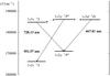 |
Fig. 1 Level diagram of the transitions between singlet states. The couplings considered in the simulations have been marked with a double arrow. |
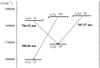 |
Fig. 2 Level diagram of the transitions between triplet states. The couplings considered in the simulations have been marked with a double arrow. |
In the numerical simulations some formal simplifications were made. Primarily, a finite number of states of the emitter atom were considered. Particulary, in this work the matrices related to the operators that appear in expressions (1) to (4) include only the states labeled in the Grotrian diagrams of Figs. 1 (singlet states) and 2 (triplet states). Furthermore, in calculating the evolution operator U(t) of each singlet or triplet we assumed that these states can be split into three groups: one upper set, which includes states n = 3, whith are coupled by the perturbing field, and two lower sets: state 1s2s and states 1s2p, which freely evolve without the influence of the perturbing field, this is called the no-quenching approximation. Thereby the matrix qR, which appears in Eq. (4), has only nonzero elements in the boxes that link the indicated states. These are the transitions marked with dashed lines in Figs. 1 and 2. On the other hand, the matrix D(t), which accounts for the optical transitions under study, only includes the transitions between states with an energy gap in the optical range, so that the transitions between states of the same group are not considered. Their radiation is beyond the optical range we studied. The fine structure was not considered, because in this study we are interested in plasmas with high and medium density, where the effects of fine structure are negligible. In Table 1 we show the energy values and transition probabilities used in the numerical calulations.
Data of the helium I atomic structure used in this work.
The plasma considered in the simulations reproduces a system of charged particles in thermodynamic equilibrium. The simulation disregards the interactions between them, in this way the particles are considered independent, and they move along straight-line trajectories with constant speed. This aproximation is acceptable in weakly coupled plasmas, as is the case for the plasmas considered in this work. For this reason, the configurations with high electron density and very low temperature must be handled with caution (in the results given here, only the plasmas with Ne ≈ 1024m-3 with T ≈ 5000K can be treated as highly coupled plasmas). The simulation volume is a spherical box in which a unique emitter is placed at rest in the center of the box, where the field generated by all particles is calculated.
To include the movement of the emitter we used the so called μ-ion model (Seidel & Stamm 1982), which considers that the velocities statistic of the relative movement between the emitter and the perturbers conform to a Maxwell-Boltzmann distribution with a perturber’s mass equal to the reduced mass of the pair emitter-perturber. With this technique we can also consider configurations that are out of thermal equilibrium between species, in which the heavy particles, ions and neutral emitters, have a lower kinetic temperature than the electrons (Gigosos et al. 2003).
The electric field experienced by the emitter and which determines the Stark-effect evolution, is obtained through a Debye potential. In this way the effect of the coupling between charges is taken into account, at least approximately. This procedure leads to a field statistics very similar to obtained in molecular dynamics simulations with interacting particles, which is much more computationally expensive (Dufour et al. 2005; Calisti et al. 2011). The details of the calculation method and the reinjection technique are reported in Gigosos & Cardeñoso (1996).
As in our previous works (Gigosos & González 2009), the differential equation of the emitter’s evolution is integrated numerically by taking the analytical solution of Eq. (4), which corresponds to a time interval Δt, the time step of the simulation, that is short enough to consider, in this time, the perturbing electric field constant. Thereby, the matrix U(t) is a succesion of products of exponential matrices. To calculate these exponentials we used a diagonalization process in each time step employing the Jacobi method (Press et al. 1997).
In our simulations, the stability and the adequacy of the statistics used were verified. Each spectrum was obtained considering between 30 000 and 60 000 samples of temporal sequences of a perturbing micro field, depending on the case considered.
2.2. Calculation results
The results of the calculations are presented in the form of tables with the FWHM and the shift of the peak as a function of electron density, temperature, and reduced mass of the pair emitter-perturber for each one of the six lines studied here. These tables are available via anonymous ftp to cdsarc.u-strasbourg.fr. The simulations were performed for the six spectral lines shown in Figs. 1 and 2 for electron density values between 1021 and 1024 m-3 with five points per decade and electron temperatures of 5000, 10 000, 20 000, 30 000, 40 000, and 60 000 K. Simulations consider different plasma compositions: helium with hydrogen ions (which leads to a reduced mass of μ = 0.8mp, where is mp being the proton mass), pure helium (μ = 2.0mp), helium with very heavy ions (μ = 4.0mp), and finally, helium in which the temperature of the heavy ions is lower than that of the electrons (μ = 10.0mp). This also allowed us to study the effects of ion dynamics.
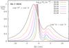 |
Fig. 3 Shape of the He I 5016 line according to the results of the simulations. The cases of high density for an electron temperature of 20 000 K in a pure helium plasma (μ = 2 in units of proton mass) are shown. The spectra are peak-normalized. |
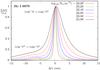 |
Fig. 4 Shape of the He I 6678 line according to the results of the simulations. The cases of high density for an electron temperature of 20 000 K in a pure helium plasma (μ = 2 in units of proton mass) are shown. The spectra are peak-normalized. |
The spectra obtained have the shape of slightly asymmetrical peaks (see the following figures). The He I 5016 and 6678 lines show a forbidden component at high densities that corresponds to the 1s3d1D → 1s2s1S transitions, for the He I 5016 line and to the 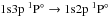 transitions, for the He I 6678 line (see Figs. 3 and 4). The forbidden components of all the other studied spectral lines are too weak and too far from the allowed peak, which renders them irrelevant. In consequence, to use them as a probe to diagnose the plasma, the full width can be enough since the shape of the spectra – apart from the lines with forbidden components mentioned before – is very close to a sligthly asymmetrical lorentzian.
In general, in the range considered within this work, the spectra have a Stark width whose dependence on the electron density N can be expressed as FWHM = f(T) Ng(N,T) with f(T) and g(N,T), certain parameters that may depend on the electron temperatue T in the first instance and depend smoothly on both T and N in the second instance.
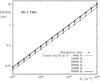 |
Fig. 5 Results of the simulations for the FWHM of the He I 7281 line. We show the data for all temperatures studied in this work for a pure helium plasma (μ = 2). These results have been fitted using mean squares to a logarithmic straight line. The fits for each set of data of a given temperature are shown. |
Figure 5 shows the FWHM of the He I 7281 line as a function of the electron density for the studied temperatures. For this spectral line it can be observed that the relation between the FWHM and N has a functional dependence on the exponent g(Ne,T) that is practically independent of the density and temperature and very close to the value g ≈ 1, as expected from spectra whose width is caused basically by electron impact (Griem 1974; Gigosos et al. 2007).
The results for the other three spectral lines are similar (not shown here). This, we insist, excludes the He I 5016 and He I 6678 lines, which at high densities behave as a spectrum with a linear Stark effect because of the proximity between the states  and 1s3d1D (see Fig. 6). These spectral lines require separate study, which is not the object of this work.
 |
Fig. 6 FWHM of the He I 5016 line as a function of the electron density in a pure helium plasma at 20 000 K. The asymptotic slopes at high and low densities are shown in a logarithmic scale to point out the weak nonlinearity between FWHM and Ne. |
2.2.1. Ion dynamic effects
The ion dynamic effects were studied in the simulations. The calculation procedure includes in a natural way the ion movement according to the μ-ion model (Seidel & Stamm 1982). The parameter μ regulates the influence of the ion movement.
The results show a slight dependence of the spectral line width on the ion movement. Table 2 shows the results of our calculations compared with the experimental data from Kobilarov et al. (1989). The value of the FWHM obtained for a pure helium plasma (μ = 2) was added as a reference in the last column. The difference between the value of the FWHM corresponding to the plasma with the experimental μ parameter and this reference value is within the experimental uncertainty range. In general, the differences in the results of the line width between the case with μ = 2.0 and the extreme cases of this work (μ = 0.8 and μ = 10) are lower than 8% for the He I 7281, He I 3889, He I 5876, and He I 7065 lines, and lower than 12% for the He I 5016 and He I 6678 lines. Therefore, in many practical cases, when the experimental uncertainty is higher than these values, this phenomenon can be omitted. However, this effect is included in all our results: the tables of FWHM and shifts, and the fitting formulas presented.
Comparison of experimental FWHM from Kobilarov et al. (1989) with the simulation results.
2.3. Fit calculation results for diagnostic purposes
With the aim of supplying a diagnostics tool for plasmas through measuring of any of the spectral lines considered in this work we performed a functional fitting of the simulation results to relate the electron density of the plasma to the full width of the spectra. We showed in Fig. 5 the relation between the two parameters that matches a linear expression on a logarithmic scale. In consequence, we adopted as a fitting function the expression  (5)We explicitly wrote the value of the power p as a constant parameter independent of the density and temperature because in the cases we treated here, there is no relevant dependence of p on these magnitudes. This simplification forces us to exclude the spectral lines from the fits whose forbidden components are noticeable even at medium densities, the He I 5016 and He I 6678 lines. For these cases, we advise using the tables provided in this work.
In the same way, the parameter A(T,μ) from (5) can be written with good accuracy as 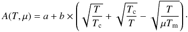 (6)The fitting parameters are a, b, Tc, and Tm. This function reproduces the simulation results quite well and is related to the influence of the magnitudes involved in it. Indeed, the effect of the electrons on the line width increases with temperature up to a certain critical value where the tendency is reversed. In the range of the study, this change cannot be appreciated for the ion dynamics since we are far away from the zone of ionic impact.
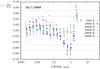 |
Fig. 7 Relative differences between the results obtained from applying the fitting formula proposed in this work and the direct data from the simulation calculation for the He I 3889 line. Difference bands of 5% and 8% are shown. |
The fitting was performed minimizing the mean square deviation between the values from the function and from the simulations, taking function (5) together with (6) and using all the data obtained from calculating the spectra. In compact form, 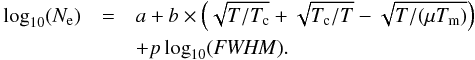 (7)Thus, a set of values (p,a,b,Tc,Tm) was obtained for every spectral line as shown in Table 3. The value of electron density, Ne, it has to be expressed in m-3, the temperature T in K, the reduced mass of the emitter-perturber pair μ in units of proton mass, and the FWHM in nm.
Direct results from the spectrum calculations and the values obtained through the fitting function differ, in general, by less than 5% (see Fig. 7 for the He I 3889 line). For He I 7281 and He I 7065 this difference reaches 8% for Ne = 1021 and 1024m-3 with T = 5000K. For the He I 3889 line, the differences reach 8% only in some cases for Ne > 1023m-3 and T < 10 000K. For the He I 5876 line, the largest differences (6%) are reached for Ne < 1022m-3 and T = 5000K. The uncertainty of the smulation results, obtained through the analysis of different sets of calculation samples, is estimated at 3%, so the quality of the fitting fomula is similar.
3. Experimental measurements
3.1. Experimental setup
In this experiment we used a small electromagnetically driven T-tube as a plasma source. The description of plasma source and experimental arrangement is given in our previous works (Djurović et al. 2005, 2009). Nevertheless, we provide some details here for completeness.
The T-tube is made of glass with an inner diameter of 27 mm. The brass reflector is placed at 140 mm from the discharge electrodes. The filling gas was pure helium at a pressure of 500 Pa. The T-tube was energized using a 4 μF capacitor bank charged to 20 kV. The block scheme of the apparatus setup is given in Fig. 8. The discharge was initiated by the 11 kV trigger pulse via the spark-gap. The discharge current was controlled by a Rogowski coil and an oscilloscope.
 |
Fig. 8 Block diagram of the T-tube experiment. |
Spectroscopic observations of plasma were made with a 1 m monochromator, an ICCD camera, and an oscilloscope. The signal from the Rogowski coil was used as trigger signal for ICCD camera. The observation point was fixed at 4 mm in front of the reflector with an exposure time of 0.5 μs. The optical signal was led to the entrance slit of the monochromator by optical fiber. The monochromator is equipped with a 1200 g/mm grating with 0.833 nm/mm inverse linear dispersion. The accuracy of the wavelength setting was 0.0025 nm. An apparatus line-broadening of 0.045 nm was obtained from lines emitted from a hollow cathode discharge. Every experimental line profile was obtained as an average profile from ten shots. The whole system, monochromator, ICCD camera, and oscilloscope were controlled by a personal computer. Particular attention was paid to a self-absorption checking test. Firstly, a standard test with the external mirror behind the plasma showed that the self-absorption effect is completely negligible under the experimental conditions mentioned above. Another test was performed. The FWHM of the He I 3889 line, which is the most intense of the considered lines, was measured with a different gas pressure and was compared with the theoretical FWHM. For this check we used independent theoretical data (Griem 1974). When the FWHM of the line was higher than the theory predicted, self-absorption was present. The results are shown in Fig. 9. The FWHM dependence of the temperature is weak.
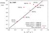 |
Fig. 9 FWHM of He I 3889 measured for different gas pressures. The simulation result at 20 000 K has been plotted. The simulation line corresponding to 10 000 K is practically the same. |
All spectral line recordings were made with 6.5 μs delay from the beginning of the discharge current, in the same way as for the whole experiment. The exception was only measurement at 200 Pa which was also made with a delay of 9.5 μs. This is shown in Fig. 9. This was made only to expand the region of measurements. It is clear from Fig. 9 that the points that represent the measured He I 3889 line FWHM follow the theoretical line for gas pressures from 200 Pa to 500 Pa. The points for higher pressures are above the theoretical line. Furthermore, the distance of the points from the theoretical line becomes larger with increasing pressure for higher pressures. This indicates that a noticeable self-absorption effect begins from a gas pressure of 550 Pa and above. Another effect can be seen from the points that correspond to pressures of 550 Pa and higher. The electron density decreases with increasing pressure. The shock wave, which produces the plasma in T-tube, becomes weaker with increasing pressure in the tube. Accordingly, we chose a gas pressure of 500 Pa for this experiment because it provides the plasma conditions with the highest electron density without a self-absorption effect.
3.2. Plasma diagnostics
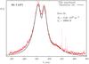 |
Fig. 10 Fit of the experimental spectra of the He I 4471 line and the result of the simulation. The electron temperature has been obtained from the result of the Boltzmann-plot with the Si II lines. The electron density of the best fit is shown. |
The electron temperature of 16 900 K was determined from the Boltzmann plot (Griem 1964) for eight Si II spectral lines. The estimated errors are within ±20%. The silicon appears like a very weak impurity of our helium plasma from the glass T-tube walls.
The electron density was obtained through several procedures. First, from the distance between the peaks of the He I 4471 according to Pérez et al. (1996), which have a value of 2.04 × 10²³m-3, or through the expression supplied by Ivković et al. (2010), which leads to a value of 2.07 × 10²³m-3. However, a comparison of the whole profile of this line to the simulation results (Gigosos & González 2009) (see Fig. 10) provides a value of 2.40 × 10²³m-3.
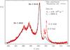 |
Fig. 11 Fit of the experimental He I 4922 line spectrum and result of the simulation. The electron temperature has been taken from the Boltzmann-plot of the Si II lines. This line overlaps with the He I 5016 line. The best fit for the He I 4922 line has been found by taking the electron density of the plasma and the relative intensities of both lines as fit parameters. The fit of He I 5016 has not been sought, it arises in a natural way from the value of Ne set by the line 4922. The two spectral lines that appear on the right side of the figure, above the forbidden component of He I 5016, arise from Silicon impurities. |
In a similar way, we fitted the data of the spectrum of He I 4922 (see Fig. 11) to the results of the simulations (Lara et al. 2012; Ivković et al. 2013), and we obtained the value 2.30 × 10²³m-3. In this last case, the fit was made including the data of He I 5016, which has been studied here.
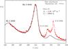 |
Fig. 12 Electron density determination using the simulation fit to the He I 5016 experimental line profile. The relative intensities of the He I 5016 and He I 4922 lines, which can be observed on the left side of the figure, are used as fit parameters. The electron temperature has been taken from the Boltzmann-plot of the Si II lines. This measurement is similar to the one represented in Fig. 11, but here the best fit with He I 5016 is sought. |
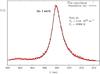 |
Fig. 13 Electron density determination using the simulation fit to the He I 6678 experimental line profile. The electron density of the plasma is used as the only fit parameter. The electron temperature has been taken from the Boltzmann-plot of the Si II lines. |
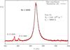 |
Fig. 14 Electron density determination using the simulation fit to the He I 3889 experimental line profile. The electron density of the plasma is used as the only fit parameter. The electron temperature has been taken from the Boltzmann-plot of the Si II lines. |
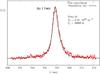 |
Fig. 15 Electron density determination using the simulation fit to the He I 7065 experimental line profile. The electron density of the plasma is used as the only fit parameter. The electron temperature has been taken from the Boltzmann-plot of the Si II lines. |
Finally, the fits of all other spectral lines considered in this work provided four additional data of the electron density (see Figs. 12 to 15). The differences between all the values obtained are less than 15%, which is a reasonable estimate of the experimental uncertainty in determining the electron density. The value adopted here is Ne = 2.34 × 10²³m-3.
Experimental FWHM and shifts obtained here.
3.3. Experimental results
The FWHM and shifts of four He I lines were measured and the results are given in Table 4. Owing to the asymmetry of the He I line profiles, the Stark shift of the lines is different when measured at the position of the peak of the line profile (dpeak) or at the middle point of the segment that shows the FWHM (d1/2). For the shift measurements we used the spectral lines emitted from the low-pressure glow discharge as unperturbed line positions. In Table 4 we list the FWHM and the shift values. The estimated experimental error for the measured FWHM is within ±12%, while for shifts it is within ±20%.
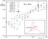 |
Fig. 16 Asymmetry parameter (the inset shows a scheme of its definition) for He I 5016. The result of this work and all results obtained in the simulations for pure helium are plotted. |
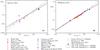 |
Fig. 20 Shift a) and FWHM b) of the He I 5016 line. The experimental and calculation data are shown. For the shift, our work is represented by two points. The small point is the shift of peak, and the large point is the shift of the half width at half maximum. |
Values of different broadening mechanisms in the experimental conditions.
The asymmetry of the spectral lines can be characterized from the difference between the values dpeak and d1/2. Figures 16 to 19 show this parameter:
 (see inset in Fig. 16 to see its meaning; λ1/2 is the wavelength of the middle point of the FWHM) as a function of the electron density for different temperatures. The data obtained in the simulation calculations and the experimental data of this work (with an estimated error bar) are plotted. It is a very noisy parameter, both for the calculation results and for the experiment results, but it allowed us to assess the differences in the detemination of the line shift for dpeak or d1/2. The main dicrepancy between the experiment and the simulation calculations can be observed in the He I 7065 line, where the experimental asymmetry is more pronounced than in the asymmetry obtained in the theory. This difference is also observed in Fig. 15, which shows both spectra.
It is well known that Stark broadening is the dominant effect for plasma conditions in this experiment. However, the contributions of other broadening mechanisms, Doppler, van der Waals, and resonance broadening, should always be checked as well as instrumental broadening. The calculated contributions for Doppler (Griem 1964), van der Waals (Griem 1964) and resonance (Ali & Griem 1965) broadening are presented in Table 5. There are no data of resonance broadening for He I 3889 and He I 7065 since these lines have no allowed transitions from either upper or lower transition energy levels to the ground state. The Doppler broadening contributes to the line FWHM in all cases by less than 3% which is deep within the experimental errors and the instrumental broadening. The other two broadening mechanisms are negligible (see Table 5). From this analysis we can conclude that the experimentally complete FWHM, appears at the same time as Stark broadening.
4. Comparison with other results
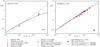 |
Fig. 21 Shift a) and FWHM b) of the He I 6678 line. The experimental and calculation data are shown. |
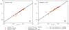 |
Fig. 22 Shift a) and FWHM b) of the He I 7281 line. The experimental and calculation data are shown. |
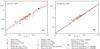 |
Fig. 23 Shift a) and FWHM b) of the He I 3889 line. The experimental and calculation data are shown. |
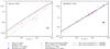 |
Fig. 24 Shift a) and FWHM b) of the He I 5876 line. The experimental and calculation data are shown. |
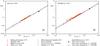 |
Fig. 25 Shift a) and FWHM b) of the He I 7065 line. The experimental and calculation data are shown. |
The theoretical and experimentally obtained Stark parameters were compared with the theoretical and experimental values reported by other authors. For the comparison, we used theoretical (Griem 1974; Bassalo et al. 1982; Sahal-Bréchot et al. 2013) and experimental data (Wulff 1958; Berg et al. 1962; Bötticher et al. 1963; Lincke 1964; Greig & Jones 1970; Kusch 1971; Morris & Cooper 1973; Mazing & Slemzin 1973; Einfeld & Sauerbrey 1975; Chiang et al. 1977; Soltwisch & Kusch 1979; Kelleher 1981; Gauthier et al. 1981; Vujičić & Kobilarov 1988; Vujičić et al. 1989; Kobilarov et al. 1989; Pérez et al. 1991, 1995; Büscher et al. 1995; Djeniže et al. 1995; Mijatović et al. 1995; Milosavljević & Djeniže 2002a,b, 2003; Pérez et al. 2003; Gao et al. 2008). The experimental data were obtained form various plasma sources with different plasma conditions and with different plasma diagnostic methods. These experimental conditions are summarized in Konjević & Roberts (1976); Konjević et al. (1984); Konjević & Wiese (1990); Konjević et al. (2002); Lesage (2009). The experimental Stark FWHM are compared in Figs. 20 to 25.
Generally, the Stark FWHM of all the four experimentally investigated lines follow a linear dependence on the electron density. All the results agree very well. The only exceptions are the FWHM results from Kusch (1971), which show higher values for He I 3889 (see Fig. 23) and lower values for He I 5016 (results not shown in Fig. 20) and the FWHM from Djeniže et al. (1995) for He I 7281.
The analytical methods included in this comparison used the standard treatment, particularly, the impact model for the electronic collisions. The difference between these two methods is mainly the manner of taking into account the close and strong collisions: through the cutoff impact parameter in Griem (1974) and Dimitrijević & Sahal-Bréchot (1990) and using a convergent theory in Bassalo et al. (1982). The simulation results agree better with the last ones. One needs to take into account that the simulations do not need any approximation to deal with the strong collisions. When a perturber is very close to the emitter, the phase change of the emission process can reach an arbitrarily high value without any divergence problem, since the computation is performed using sinusoidal functions of the electric field module (arbitrarily high). The numerical calculation does not present any divergences, because the numerical integration was made considering the interaction between the emitter and the perturber without any approximation. For practical purposes, this phase change represents a total breakdown of the emitter coherence, so that the exact results from the simulations fit to the old Lorentz model very well.
A much smaller number of experimental Stark shift data is available. Kobilarov et al. (1989) reported only a shift increment for electron densities between 6.1 × 10²² and 9.8 × 10²²m-3, and these results are not included in this consideration. Some authors, for example Berg et al. (1962); Bötticher et al. (1963); Lincke (1964); Greig & Jones (1970) reported shifts measured at peak positions while others (Kelleher 1981; Gauthier et al. 1981; Vujičić & Kobilarov 1988; Vujičić et al. 1989; Kobilarov et al. 1989; Pérez et al. 1991; Djeniže et al. 1995; Mijatović et al. 1995) reported shifts measured at the half-width level position. We presented the experimentally obtained shift values in Figs. 20 to 25. Even the mixed shift values are presented in the graphs, and even the shift experimental errors are always larger than those of the FWHM; a clear linear tend for the electron density can be observed. Only the results of Djeniže et al. (1995) a slightly deviate from this trend for He I 5016. As we mentioned above, the two lines with noticeable forbidden components deviate from the ideal linear trend.
Naturally, the characteristic time of the dynamic of the electronic fields is much lower than the loss the correlation time of the emitter dipole at very low densities, when the typical Stark effect is very weak and the lines are narrow. Under these circumstances, the considerations of the impact model are very convenient (Gigosos et al. 2007) and the simulations perfectly reproduce that situation: the width and the shift of the lines are linear with the electron density and fit to the so-called impact limit.
5. Conclusions
We reported Stark parameters calculated for six and measured for four He I spectral lines. The obtained Stark parameters were compared with other available experimental and theoretical data. All Stark FWHM results agree very well although they were obtained under different plasma conditions. The linear trend of the FWHM versus electron density for four out of the six studied spectral lines is very clear.
We conclude that the Stark FWHM of all six considered lines can be used as very good tool for electron density determinations in a wide region of electron densities.
Acknowledgments
The Spanish group thanks the Spanish Ministerio de Ciencia e Inovación for its support under contract no ENE2010-19542/FTN. D. González-Herrero stayed in Novi Sad, funded by the Spanish Ministerio de Ciencia e Inovación (grant no BES-2011-046770). S. Djurović, I. Savić, Z. Mijatović and R. Kobilarov thank the Ministry of Education, Science and Technological Development of the Republic of Serbia for support via Project 171014.
References
- Ali, A. W., & Griem, H. R. 1965, Phys. Rev., 140, 1044 [NASA ADS] [CrossRef] [Google Scholar]
- Ali, A. W., & Griem, H. R. 1966, Phys. Rev., 144, 366 [NASA ADS] [CrossRef] [Google Scholar]
- Anderson, P. W. 1949, Phys. Rev., 76, 647 [NASA ADS] [CrossRef] [Google Scholar]
- Bassalo, J. M., Cattani, M., & Walder, V. S. 1982, J. Quant. Spectr. Rad. Transf., 28, 75 [Google Scholar]
- Berg, H. F., Ali, A. W., Lincke, R., & Griem, H. R. 1962, Phys. Rev., 125, 199 [NASA ADS] [CrossRef] [Google Scholar]
- Bötticher, W., Roder, O., & Wobig, K. H. 1963, Z. Phys., 175, 480 [Google Scholar]
- Büscher, S., Glenzer, S., Wrubel, T. H., & Kunze, H.-J. 1995, J. Quant. Spectr. Rad. Transf., 54, 73 [Google Scholar]
- Calisti, A., Ferri, S., Mossé, C., et al. 2011, High Energy Density Physics, 7, 197 [NASA ADS] [CrossRef] [Google Scholar]
- Chiang, W. T., Murphy, D. P., Chen, Y. G., & Griem, H. R. 1977, Z. Naturforsch., 32, 818 [NASA ADS] [Google Scholar]
- Djeniže, S., Skuljan, L., & Konjević, N. 1995, J. Quant. Spectr. Rad. Transf., 54, 581 [NASA ADS] [CrossRef] [Google Scholar]
- Djurović, S., Nikolić, D., Savić, I., Sörge, S., & Demura, A. V. 2005, Phys. Rev. E, 71, 036407 [NASA ADS] [CrossRef] [Google Scholar]
- Djurović, S., Ćirišan, M., Demura, A. V., et al. 2009, Phys. Rev. E, 79, 046402 [NASA ADS] [CrossRef] [Google Scholar]
- Dimitrijević, M. S., & Sahal-Bréchot, S. 1990, A&ASS, 82, 519 [NASA ADS] [Google Scholar]
- Dufour, E., Calisti, A., & Talin, B. 2005, Phys. Rev. E, 71, 066409 [NASA ADS] [CrossRef] [Google Scholar]
- Einfeld, D., & Sauerbrey, G. 1975, Z. Naturforsch., 31a, 310 [Google Scholar]
- Gao, H. M., Ma, S. L., Xu, C. M., & Wu, L. 2008, Eur. Phys. J. D, 47, 191 [NASA ADS] [CrossRef] [EDP Sciences] [Google Scholar]
- Gauthier, J. C., Geindre, J. P., Goldbach, C., et al. 1981, J. Phys. B, 14, 2099 [Google Scholar]
- Geier, S., Heber, U., Heuser, C., et al. 2013, A&A, 551, L4 [NASA ADS] [CrossRef] [EDP Sciences] [Google Scholar]
- Gigosos, M. A., & Cardeñoso, V. 1996, J. Phys. B, 29, 4795 [Google Scholar]
- Gigosos, M. A., & González, M. Á. 2009, A&A, 503, 293 [NASA ADS] [CrossRef] [EDP Sciences] [Google Scholar]
- Gigosos, M. A., González, M. Á., & Cardeñoso, V. 2003, Spectrochim. Acta B, 58, 1489 [Google Scholar]
- Gigosos, M. A., González, M. Á., Talin, B., & Calisti, A. 2007, A&A, 466, 1189 [NASA ADS] [CrossRef] [EDP Sciences] [Google Scholar]
- Greig, J. R., & Jones, L. A. 1970, Phys. Rev. A, 1, 1261 [NASA ADS] [CrossRef] [Google Scholar]
- Griem, H. R. 1964, Plasma Spectroscopy (New York: McGraw-Hill) [Google Scholar]
- Griem, H. R. 1974, Spectral Line Broadening by Plasmas (New York: Academic Press) [Google Scholar]
- Iijima, T., & Cassatella, A. 2010, A&A, 516, A54 [NASA ADS] [CrossRef] [EDP Sciences] [Google Scholar]
- Ivković, M., González, M. Á., Jovićević, S., Gigosos, M. A., & Konjević, N. 2010, Spectrochim. Acta B, 65, 234 [NASA ADS] [CrossRef] [Google Scholar]
- Ivković, M., González, M. Á., Lara, N., Gigosos, M. A., & Konjević, N. 2013, J. Quant. Spectr. Rad. Transf., 127, 82 [NASA ADS] [CrossRef] [Google Scholar]
- Kelleher, D. E. 1981, J. Quant. Spectr. Rad. Transf., 25, 191 [Google Scholar]
- Kobilarov, R., Konjević, N., & Popović, M. V. 1989, Phys. Rev. A, 40, 3871 [NASA ADS] [CrossRef] [PubMed] [Google Scholar]
- Konjević, N., & Roberts, J. R. 1976, J. Phys. Chem. Ref. Data, 5, 209 [NASA ADS] [CrossRef] [Google Scholar]
- Konjević, N., & Wiese, W. L. 1990, J. Phys. Chem. Ref. Data, 19, 1307 [Google Scholar]
- Konjević, N., Dimitrijević, M. S., & Wiese, W. L. 1984, J. Phys. Chem. Ref. Data, 13, 619 [NASA ADS] [CrossRef] [Google Scholar]
- Konjević, N., Lesage, A., Fuhr, R., & Wiese, W. L. 2002, J. Phys. Chem. Ref. Data, 31, 819 [NASA ADS] [CrossRef] [Google Scholar]
- Kusch, H. J. 1971, Z. Naturforsch. A, 26, 1970 [NASA ADS] [Google Scholar]
- Lara, N., González, M. Á., & Gigosos, M. A. 2012, A&A, 542, A75 [NASA ADS] [CrossRef] [EDP Sciences] [Google Scholar]
- Léger, L., & Paletou, F. 2009, A&A, 498, 869 [NASA ADS] [CrossRef] [EDP Sciences] [Google Scholar]
- Leighly, K. M., Dietrich, M., & Barber, S. 2011, ApJ, 728, 94 [NASA ADS] [CrossRef] [Google Scholar]
- Lesage, A. 2009, New Astron. Rev., 52, 471 [NASA ADS] [CrossRef] [Google Scholar]
- Lincke, R. 1964, Ph.D. Thesis, University of Maryland, USA [Google Scholar]
- Mazing, M. A., & Slemzin, V. A. 1973, Sov. Phys. Lebedev Inst. Rep., 4, 42 [Google Scholar]
- Mijatović, Z., Konjević, N., Ivković, M., & Kobilarov, R. 1995, Phys. Rev. E, 51, 4891 [Google Scholar]
- Milosavljević, V., & Djeniže, S. 2002a, A&A, 393, 721 [NASA ADS] [CrossRef] [EDP Sciences] [Google Scholar]
- Milosavljević, V., & Djeniže, S. 2002b, New Astron., 7, 543 [NASA ADS] [CrossRef] [Google Scholar]
- Milosavljević, V., & Djeniže, S. 2003, Eur. Phys. J. D, 23, 385 [NASA ADS] [CrossRef] [EDP Sciences] [Google Scholar]
- Monfared, S. K., Graham, W. G., Morgan, T. J., & Huwel, L. 2011, Plasma Sources Sci. T., 20, 035001 [NASA ADS] [CrossRef] [Google Scholar]
- Morris, R. N., & Cooper, J. 1973, Can. J. Phys., 51, 1746 [NASA ADS] [CrossRef] [Google Scholar]
- Parigger, C. G. 2013, Spectrochim. Acta B, 79, 4 [NASA ADS] [CrossRef] [Google Scholar]
- Peach, G., Dimitrijevic, M. S., & Phillip, C. S. 2009, Trans. IAU, 4, 385 [Google Scholar]
- Pérez, C., de la Posa, I., de Frutos, A. M., & Mar, S. 1991, Phys. Rev. A, 44, 6785 [Google Scholar]
- Pérez, C., Aparicio, J. A., de la Rosa, I., Mar, S., & Gigosos, M. A. 1995, Phys. Rev. E, 51, 3764 [NASA ADS] [CrossRef] [Google Scholar]
- Pérez, C., de la Rosa, I., Aparicio, J. A., Mar, S., & Gigosos, M. A. 1996, Jpn J. Appl. Phys., 35, 4073 [Google Scholar]
- Pérez, C., Santamarta, R., de la Rosa, I., & Mar, S. 2003, Eur. Phys. J. D, 27, 73 [NASA ADS] [CrossRef] [EDP Sciences] [Google Scholar]
- Press, W. W., Teukolsky, S. A., Vetterling, W. T., & Flannery, B. P. 1997, Numerical Recipes in C (New York: Cambridge University Press) [Google Scholar]
- Sahal-Bréchot, S., Dimitrijevic, M. S., & Moreau, N. 2013, STARK-B database (Observatory of Paris, LERMA and Astronomical Observatory of Belgrade), Available: http://stark-b.obspm.fr (see Dimitrijević & Sahal-Bréchot 1990) [Google Scholar]
- Seidel, J., & Stamm, R. 1982, J. Quant. Spectr. Rad. Transf., 27, 499 [Google Scholar]
- Soltwisch, H., & Kusch, H. J. 1979, Z. Naturforsch., 34, 300 [NASA ADS] [Google Scholar]
- Takaki, K., Kawabata, K. S., Yamanaka, M., et al. 2013, Astrophys. Lett. Comm., 722, L17 [Google Scholar]
- Thompson, G. B., & Morrison, N. D. 2013 AJ, 145, 95 [NASA ADS] [CrossRef] [Google Scholar]
- Vujičić, B. T., & Kobilarov, R. 1988, 9th Int. Conf. Spectral Line Shapes, Contributed papers (Torun, Poland: Nicolas Copernicus University Press), 18 [Google Scholar]
- Vujičić, B. T., Djurović, S., & Halenka, J. 1989, Z. Phys. D, 11, 119 [NASA ADS] [Google Scholar]
- Wahlgren, G. M., van Dishoeck, E. F., Federman, S. R., et al. 2012, Trans. IAU, 7, 339 [Google Scholar]
- Wolff, B., Koester, D., Montgomery, M. H., & Winget, D. E. 2002, A&A, 388, 320 [NASA ADS] [CrossRef] [EDP Sciences] [Google Scholar]
- Wulff, H. 1958, Z. Phys., 150, 614 [Google Scholar]
All Tables
Comparison of experimental FWHM from Kobilarov et al. (1989) with the simulation results.
All Figures
|
Fig. 1 Level diagram of the transitions between singlet states. The couplings considered in the simulations have been marked with a double arrow. |
| In the text | |
|
Fig. 2 Level diagram of the transitions between triplet states. The couplings considered in the simulations have been marked with a double arrow. |
| In the text | |
|
Fig. 3 Shape of the He I 5016 line according to the results of the simulations. The cases of high density for an electron temperature of 20 000 K in a pure helium plasma (μ = 2 in units of proton mass) are shown. The spectra are peak-normalized. |
| In the text | |
|
Fig. 4 Shape of the He I 6678 line according to the results of the simulations. The cases of high density for an electron temperature of 20 000 K in a pure helium plasma (μ = 2 in units of proton mass) are shown. The spectra are peak-normalized. |
| In the text | |
|
Fig. 5 Results of the simulations for the FWHM of the He I 7281 line. We show the data for all temperatures studied in this work for a pure helium plasma (μ = 2). These results have been fitted using mean squares to a logarithmic straight line. The fits for each set of data of a given temperature are shown. |
| In the text | |
|
Fig. 6 FWHM of the He I 5016 line as a function of the electron density in a pure helium plasma at 20 000 K. The asymptotic slopes at high and low densities are shown in a logarithmic scale to point out the weak nonlinearity between FWHM and Ne. |
| In the text | |
|
Fig. 7 Relative differences between the results obtained from applying the fitting formula proposed in this work and the direct data from the simulation calculation for the He I 3889 line. Difference bands of 5% and 8% are shown. |
| In the text | |
|
Fig. 8 Block diagram of the T-tube experiment. |
| In the text | |
|
Fig. 9 FWHM of He I 3889 measured for different gas pressures. The simulation result at 20 000 K has been plotted. The simulation line corresponding to 10 000 K is practically the same. |
| In the text | |
|
Fig. 10 Fit of the experimental spectra of the He I 4471 line and the result of the simulation. The electron temperature has been obtained from the result of the Boltzmann-plot with the Si II lines. The electron density of the best fit is shown. |
| In the text | |
|
Fig. 11 Fit of the experimental He I 4922 line spectrum and result of the simulation. The electron temperature has been taken from the Boltzmann-plot of the Si II lines. This line overlaps with the He I 5016 line. The best fit for the He I 4922 line has been found by taking the electron density of the plasma and the relative intensities of both lines as fit parameters. The fit of He I 5016 has not been sought, it arises in a natural way from the value of Ne set by the line 4922. The two spectral lines that appear on the right side of the figure, above the forbidden component of He I 5016, arise from Silicon impurities. |
| In the text | |
|
Fig. 12 Electron density determination using the simulation fit to the He I 5016 experimental line profile. The relative intensities of the He I 5016 and He I 4922 lines, which can be observed on the left side of the figure, are used as fit parameters. The electron temperature has been taken from the Boltzmann-plot of the Si II lines. This measurement is similar to the one represented in Fig. 11, but here the best fit with He I 5016 is sought. |
| In the text | |
|
Fig. 13 Electron density determination using the simulation fit to the He I 6678 experimental line profile. The electron density of the plasma is used as the only fit parameter. The electron temperature has been taken from the Boltzmann-plot of the Si II lines. |
| In the text | |
|
Fig. 14 Electron density determination using the simulation fit to the He I 3889 experimental line profile. The electron density of the plasma is used as the only fit parameter. The electron temperature has been taken from the Boltzmann-plot of the Si II lines. |
| In the text | |
|
Fig. 15 Electron density determination using the simulation fit to the He I 7065 experimental line profile. The electron density of the plasma is used as the only fit parameter. The electron temperature has been taken from the Boltzmann-plot of the Si II lines. |
| In the text | |
|
Fig. 16 Asymmetry parameter (the inset shows a scheme of its definition) for He I 5016. The result of this work and all results obtained in the simulations for pure helium are plotted. |
| In the text | |
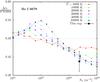 |
Fig. 17 Asymmetry parameter (see Fig. 16) for He I 6689. |
| In the text | |
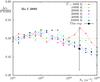 |
Fig. 18 Asymmetry parameter (see Fig. 16) for He I 3889. |
| In the text | |
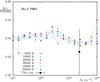 |
Fig. 19 Asymmetry parameter (see Fig. 16) for He I 7065. |
| In the text | |
|
Fig. 20 Shift a) and FWHM b) of the He I 5016 line. The experimental and calculation data are shown. For the shift, our work is represented by two points. The small point is the shift of peak, and the large point is the shift of the half width at half maximum. |
| In the text | |
|
Fig. 21 Shift a) and FWHM b) of the He I 6678 line. The experimental and calculation data are shown. |
| In the text | |
|
Fig. 22 Shift a) and FWHM b) of the He I 7281 line. The experimental and calculation data are shown. |
| In the text | |
|
Fig. 23 Shift a) and FWHM b) of the He I 3889 line. The experimental and calculation data are shown. |
| In the text | |
|
Fig. 24 Shift a) and FWHM b) of the He I 5876 line. The experimental and calculation data are shown. |
| In the text | |
|
Fig. 25 Shift a) and FWHM b) of the He I 7065 line. The experimental and calculation data are shown. |
| In the text | |
Current usage metrics show cumulative count of Article Views (full-text article views including HTML views, PDF and ePub downloads, according to the available data) and Abstracts Views on Vision4Press platform.
Data correspond to usage on the plateform after 2015. The current usage metrics is available 48-96 hours after online publication and is updated daily on week days.
Initial download of the metrics may take a while.