| Issue |
A&A
Volume 561, January 2014
|
|
|---|---|---|
| Article Number | A148 | |
| Number of page(s) | 12 | |
| Section | Interstellar and circumstellar matter | |
| DOI | https://doi.org/10.1051/0004-6361/201322310 | |
| Published online | 28 January 2014 | |
The mass distribution of clumps within infrared dark clouds. A Large APEX Bolometer Camera study⋆,⋆⋆
1 Departamento de Astronomía, Universidad de Chile, Camino El Observatorio 1515, Las Condes, 36D Casilla, Santiago, Chile
e-mail: This email address is being protected from spambots. You need JavaScript enabled to view it.
2 Max-Planck-Institut für Radioastronomie, Auf dem Hügel 69, 53121 Bonn, Germany
e-mail: This email address is being protected from spambots. You need JavaScript enabled to view it.
; This email address is being protected from spambots. You need JavaScript enabled to view it.
3 CSIRO Astronomy and Space Science, PO Box 76, NSW 1710 Epping, Australia
4 European Southern Observatory, Alonso de Córdova 3107, Vitacura, 19001 Casilla, 19 Santiago, Chile
e-mail: This email address is being protected from spambots. You need JavaScript enabled to view it.
5 Centro de Radioastronomía y Astrofísica, Universidad Nacional Autónoma de México, Apdo. Postal 3–72, 58090 Morelia, Michoacán, México
e-mail: This email address is being protected from spambots. You need JavaScript enabled to view it.
Received: 18 July 2013
Accepted: 27 November 2013
Abstract
Aims. We present an analysis of the dust continuum emission at 870 μm in order to investigate the mass distribution of clumps within infrared dark clouds (IRDCs).
Methods. We map six IRDCs with the Large APEX BOlometer CAmera (LABOCA) at APEX, reaching an rms noise level of σrms = 28–44 mJy beam-1. The dust continuum emission coming from these IRDCs was decomposed by using two automated algorithms, Gaussclumps and Clumpfind. Moreover, we carried out single-pointing observations of the N2H+ (3–2) line toward selected positions to obtain kinematic information.
Results. The mapped IRDCs are located in the range of kinematic distances of 2.7–3.2 kpc. We identify 510 and 352 sources with Gaussclumps and Clumpfind, respectively, and estimate masses and other physical properties assuming a uniform dust temperature. The mass ranges are 6–2692 M⊙ (Gaussclumps) and 7–4254 M⊙ (Clumpfind), and the ranges in effective radius are ~0.10–0.74 pc (Gaussclumps) and 0.16–0.99 pc (Clumpfind). The mass distribution, independent of the decomposition method used, is fitted by a power law, dN/dM ∝ Mα, with an index (α) of −1.60 ± 0.06, consistent with the CO mass distribution and other high-mass star-forming regions.
Key words: stars: formation / ISM: clouds / dust, extinction / submillimeter: ISM
Based on data acquired with the Atacama Pathfinder Experiment (APEX). APEX is a collaboration between the Max-Planck-Institut für Radioastronomie, the European Southern Observatory, and the Onsala Space Observatory.
Full Tables 3 and 4 are only available at the CDS via anonymous ftp to cdsarc.u-strasbg.fr (130.79.128.5) or via http://cdsarc.u-strasbg.fr/viz-bin/qcat?J/A+A/561/A148
© ESO, 2014
1. Introduction
Stars form in the densest parts of molecular clouds. The mass distribution (dN/dM ∝ Mα) of dense clumps, which is obtained from observations of lines from the CO and CS molecules, is a power law with an index of α ~ −1.7 (e.g., Lada et al. 1991; Blitz 1993; Kramer et al. 1998). Continuum observations of high-mass star-forming regions (HMSFRs) in the millimeter regime have also revealed indices of α ~ −1.7 (e.g., Mookerjea et al. 2004; Muñoz et al. 2007; López et al. 2011). When studying the mass distributions of lower mass dense cores, some authors have found a steeper value for the slope of that distribution (α ~ −2.3; e.g., Belloche et al. 2011), resembling the index of the stellar initial mass function (IMF), i.e., α = −2.35 (Salpeter 1955). Similar values have been claimed for the mass distributions of embedded, open, and globular clusters (e.g, Elmegreen & Efremov 1997; Lada & Lada 2003). These similarities might imply that the form of the mass distribution is carried from the interstellar matter to stars. However, the origin of the mass distribution is still a matter of debate, and some authors have disputed its universality (e.g., Bastian et al. 2010; Hsu et al. 2010; Weidner et al. 2010).
Several studies reveal that some clumps within the so-called infrared dark clouds (IRDCs) harbor the earliest stages of HMSF (e.g., Rathborne et al. 2006; Battersby et al. 2010). Therefore, IRDCs are good candidates for studying the mass distribution of their clumps/cores. Different studies of the mass distributions of IRDCs based on either extinction or continuum maps and different assumptions, e.g., source extraction, mass estimation, etc., find a range of indices from α ~ −1.7 to −2.1 (e.g., Rathborne et al. 2006; Ragan et al. 2009; Peretto & Fuller 2010; Miettinen 2012).
Here we aim at studying the mass distribution of clumps within six IRDCs in the dust continuum emission at 870 μm that are located at kinematic distances of 2.7–3.2 kpc. In Sect. 2, we present the IRDC sample, dust continuum emission observations, and molecular line (N2H+ 3–2) observations. Section 3 shows the resulting dust emission maps and sample spectra, while Sect. 4 presents the source decomposition analysis, the mass-radius relationship, and the clump mass distribution. The results are discussed in Sect. 5 and, finally, we summarize our findings in Sect. 6.
We adopt a nomenclature in which clumps refer to structures with diameters of ~1 pc, embedded within a cloud (of several pc), and cores refer to structures within a clump with diameters of ~0.1 pc.
2. Observations and data reduction
2.1. Continuum data
We selected six southern hemisphere clouds with high contrast, i.e., high extinction, from our IRDC catalog at 24 μm, which was created by applying the method from Simon et al. (2006a) to Spitzer/MIPSGAL images (Carey et al. 2009). In Table 1 we list the IRDCs observed with LABOCA on the APEX 12 m telescope (Güsten et al. 2006). LABOCA, the Large APEX BOlometer CAmera (Siringo et al. 2009), is a bolometer array of 295 pixels working at 870 μm (345 GHz), a bandwidth of about 60 GHz, and a field of view of 114. The LABOCA instrument was developed by the Max-Planck-Institut für Radioastronomie.
The observations were performed on 2007 August 25 and 27−28, typically covering an area of ~20′ × 20′ for each IRDC. The sky opacity was determined every one to two hours with skydips. The focus was optimized on Jupiter. Pointing observations were checked on the source IRAS 16293−2422 (see Appendix A of Siringo et al. 2009), and the telescope pointing was found to be accurate to within 5′′.
We used the Bolometer array data Analysis package (BoA; Schuller 2012) to reduce the LABOCA data. The data reduction involves flux calibration, flagging bad and noisy pixels, removal of correlated noise, despiking, low-frequency filtering, and first-order baseline removal. These procedures are explained in detail in Siringo et al. (2009) and Schuller et al. (2009). The removal of correlated noise was done on all pixels with the median noise method with five iterations and a relative gain of 0.8. The correlated noise for the pixels sharing the same electronics subsystem was removed with two iterations and a relative gain of 0.8. The same numbers of iterations and gain were applied to groups of pixels connected to the same read-out cable.
Each map was built using natural weighting, where each data point has a weight 1/ and where σi is the standard deviation of each pixel. The resulting map after performing the whole process was used as a model for the next iteration. A total of 20 iterations were performed. As shown in Belloche et al. (2011), this iterative process helps to recover flux at each iteration and to recover extended emission. Still, it is important to point out that the spatial filtering due to the correlated noise removal can reduce the sizes of extended structures. Belloche et al. (2011) also find that the size for their (input artificial) circular sources with sizes from 200′′ to 440′′ are reduced by 15% to 50%, while for elliptical sources with aspect ratio of 2.5 and minor axis (FWHM) varying from 19
 2 to 222′′, the sizes are reduced by 20–25%.
The final flux calibration is accurate to ~20%. The data were projected on maps with a pixel size of one third of the beam full width at half maximum (FWHM) and the map in the last iteration was smoothed with a Gaussian kernel of 10′′, providing a resolution of the final map of 216, which corresponds to 0.30 pc at a distance of 2.9 kpc. The rms noise level (σrms) varies from IRDC to IRDC between 28 and 44 mJy beam-1 (see Table 1). In comparison to the APEX Telescope Large Area Survey of the Galaxy (ATLASGAL), also at 870 μm (Schuller et al. 2009), our observations go deeper by about a factor of 2, which as we see in the next sections, helps probe a wider mass range.
Pointing centers of IRDCs observed with LABOCA.
2.2. Molecular line data
In addition to the continuum data, we performed N2H+ (3–2) line observations with the double-sideband heterodyne receiver APEX-2A (Risacher et al. 2006) toward selected positions in order to obtain kinematic distances. In total, 18 positions were observed within the six IRDCs, typically with two to five pointings per cloud. These IR-quiet and IR-loud targets were chosen by eye from Spitzer/GLIMPSE images at 8 μm. Table 2 lists the observed positions and includes whether the target is dark at 8 μm and at 24 μm.
Observations were carried out with the APEX telescope on 2007 October 28-29. The fast Fourier transform spectrometer (FFTS; Klein et al. 2006) was used as a backend for these observations. The pointing was checked on the core G327.3-0.6 and the source 18592+0109 every hour. System temperature varied from 201 to 243 K. N2H+ (3–2) line parameters12 are ν = 279511.7348 MHz, Eu/k = 26.83 K, HPBW = 22′′, Beff = 0.73, Feff = 0.95, and δvres = 0.52 km s-1.
The data was reduced with the CLASS program from the GILDAS package3. We summed up individual scans and fitted and subtracted a polynomial of order 1 or 2 to the baseline of each final spectrum. For several spectra that were affected by standing waves in the optics (between the subreflector and the receiver) or by an instability of the receiver itself, we edited and performed a linear interpolation on the Fourier transform to remove the sinusoidal pattern. The conversion from  to TMB was done with the efficiencies mentioned before.
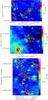 |
Fig. 1 Contour maps obtained with LABOCA at 870 μm overlaid on the Spitzer/MIPSGAL 24 μm images for the IRDCs G329 (top), G331 (middle), and G335 (bottom). The beam HPBW (21 |
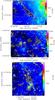 |
Fig. 2 Same as Fig. 1 but for the IRDCs G337 (top), G343 (middle), and G345 (bottom). Contours for G337 are 3, 6, 12, 24, 48, 96, 192 times 0.031 Jy beam-1, the rms noise of the image. Contours for G343 are 3, 6, 12, 24, 48, 96 times 0.028 Jy beam-1, the rms noise of the image. Contours for G345 are 3, 6, 12, 24, 48, 96, 192, 384 times 0.037 Jy beam-1, the rms noise of the image. |
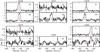 |
Fig. 3 APEX2A spectra (histograms) of the N2H+ (3–2) line. The red solid lines indicate the relative intensities for each of the 29 hyperfine components. P labels refer to the positions marked in Figs. 1 and 2 with red stars. |
N2H+ (3–2) observational parameters, distances, and virial masses.
3. Observational results
Figures 1 and 2 show the final maps obtained with LABOCA in contours overlaid on Spitzer/MIPSGAL 24 μm images. The mapped regions show extended, filamentary, and compact dust continuum emission. The prominent features are those associated with bright 24 μm sources. Filamentary IR-dark structures in the 24 μm images can be seen in dust emission at 870 μm extending for more than 10′ (~9 pc at a distance of 2.7 kpc). All clouds show several compact sources. Some of these compact sources are shrouded in the filamentary emission while others surround the extended structures.
In general, there is good correlation between the 24 μm dark structures and the emission at 870 μm, but there are some IR-dark patches that do not have a submillimeter emission counterpart. IRDCs G343 and G345 seem to be more fragmented than the others and present emission all over the field contrary to, say IRDCs G329 and G331. We see clouds that are connected/linked by an envelope, e.g., IRDCs G337 and G331; clouds with clear compact sources still embedded in the envelope, e.g., IRDCs G329 and G335; and clouds that are more dispersed over the mapped regions, e.g., IRDCs G343 and G345.
Sample spectra of the N2H+ (3–2) line toward positions where emission was detected are shown in Fig. 3. Gaussian fits results are listed in Table 2; we detected emission in 11 sources and the average 1σrms noise level for non-detections was ~0.24 K. The line widths obtained with the hyperfine structure fitting procedure of CLASS (“method HFS”) are narrower than those obtained with Gaussian fits, up to 50% in two clumps (G331P2 and G345P1). In these two cases, we obtained very high optical depths (~13). The hyperfine components of N2H+ are also plotted in Fig. 3.
Sources found with Gaussclumps and derived physical parameters.
4. Analysis
4.1. Molecular line data
The “near” kinematic distances (see Table 2) are estimated based on the Galactic rotation curve model by Fich et al. (1989), assuming the IAU standard rotation constants of distance to the Sun from the Galactic center as R0 = 8.5 kpc and the Sun’s rotation speed around the Galactic center as Θ0 = 220 km s-1. In the calculations, we use the LSR velocity of N2H+ (3–2). In all clouds, except one, we have two detections of N2H+ (3–2). The difference in the LSR velocities of the clumps will result in a distance difference of up to 0.2 kpc, but this difference is easily explained by velocity variations within the parental molecular clouds.
4.2. Source extraction from continuum maps: Gaussclumps and Clumpfind
We use the two most popular algorithms Gaussclumps (Stutzki & Guesten 1990; Kramer et al. 1998) and Clumpfind (Williams et al. 1994) to extract clumps and derive their physical properties from the dust emission.
Gaussclumps, a task in the GILDAS4 package, was originally written to decompose a three-dimensional data cube into Gaussian-shaped sources (see Stutzki & Guesten 1990) but can also be applied to dust continuum maps (e.g., Mookerjea et al. 2004). Two adjacent empty planes were added to the original two-dimensional maps needed for the algorithm to run properly. “Stiffness” parameters that control the fitting, ensuring that a local clump is fitted and subtracted, were set to 1 (Kramer et al. 1998). A peak flux density threshold was set to 5σrms. Following Belloche et al. (2011), the initial guesses for the aperture cutoff, the aperture FWHM and the source FWHM were set to 8, 3, and 1.5 times the angular resolution, respectively.
The resulting Gaussian sources derived from Gaussclumps are listed in Table 3. Columns are (1) region name, (2) running number in the order Gaussclumps finds the source, (3)–(4) J2000 position, (5) peak intensity, (6) flux density, (7)–(8) angular FWHM along the major and minor axes determined from Gaussian fits before deconvolution, (9)–(10) deconvolved FWHMs (sizes smaller than 25.9′′ were set to 25.9′′ to compute the deconvolved sizes, in order to account for a fit inaccuracy corresponding to a 5-σrms detection in peak intensity), (11) position angle, (12) deconvolved effective radius, Reff, (13)–(15) total mass derived from the Gaussian fit, beam-averaged H2 column density, NH2, and volume density, nH2 (see Sect. 4.3). Sources lying on noisy edges were discarded from further analysis. IRDCs G329, G331, G335, G337, G343, and G345 were decomposed into 75, 41, 123, 65, 83, and 123 Gaussian sources, respectively, in a total of 510 sources.
Clumpfind, unlike Gaussclumps, needs only two parameters (threshold and stepsize) to identify clumps. The program clfin2d5 is a modification of the original code for three-dimensional datacubes. We start the contouring at 3σrms (threshold) with an interval of 2σrms (stepsize) to process each dust emission map. As Pineda et al. (2009) have found, the number of identified sources depends on the combination of chosen threshold and stepsize. As the stepsize decreases, the number of clumps increases.
All the emission is assigned to clumps above the given threshold. It is important to point out that Clumpfind does not assume Gaussian shape and does not allow overlapping of identified sources. Sources identified by Clumpfind are listed in Table 4. Columns are (1) region name; (2) running number in the order Clumpfind finds the source; (3)–(4) J2000 position; (5) peak intensity; (6) flux density; (7) deconvolved effective radius; (8)–(10) total mass, beam-averaged H2 column density, and volume density (see Sect. 4.3). IRDCs G329, G331, G335, G337, G343, and G345 were decomposed into 39, 33, 84, 53, 63, and 80 sources, respectively, in total, 352 sources.
Sources found with Clumpfind and derived physical parameters.
We do not find a one-to-one correspondence for all Gaussclumps and Clumpfind sources. In each cloud, Gaussclumps decomposes emission into more and smaller sources than Clumpfind does, especially around very bright dust peaks.
4.3. Gas and virial mass, column density, and volume density estimates
For each identified source and for both methods, we estimated the gas mass (M), assuming that the submillimeter emission is optically thin, according to the expression (Hildebrand 1983) 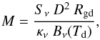 (1)where Sν is the observed integrated flux density, D the distance, Rgd the gas-to-dust mass ratio, κν the dust opacity coefficient, and Bν(Td) the Planck function at the dust temperature (Td). We assume a gas-to-dust mass ratio of 100 and adopt a κν = 1.95 cm2 g-1 (interpolated to 870 μm from Table 1, Col. 9 of Ossenkopf & Henning 1994), for an MRN (Mathis et al. 1977) graphite-silicate grain mixture with thick ice mantles, at a gas density of 106 cm-3. In the case of the IRDC G343, whose rms noise is the lowest, and assuming Td = 18 K, the detection limit is ~4 M⊙ with Sν = 0.084 Jy (3σrms detection level), at a distance of 2.7 kpc.
We use Td = 18 K to compute the masses presented in Tables 3 and 4. This temperature is in accordance with previous works toward IRDCs (e.g., Pillai et al. 2006; Rathborne et al. 2010; Miettinen 2012). Rathborne et al. (2010) estimated dust temperatures for 190 cores within IRDCs by doing graybody fits to their spectral energy distributions (SEDs). They obtain median values that range between 23.7 ± 5.3 and 40.4 ± 5.7 K. We are aware that our assumption of low temperature is not valid for sources that are associated with masers, HII regions, UCHII regions, and/or IRAS/MSX/24 μm point sources, namely regions with signs of active star formation (see Sect. 4.4), whose temperature should be higher. On the other hand, sources not associated with any of those star formation signposts are expected to have a lower temperature. We note that by decreasing the temperature from 18 K to 12 K, the mass would almost double, while with an increase from 18 K to 30 K, the mass would decrease by 50%.
Using the N2H+ (3–2) FWHM line widths (ΔV), we estimate the virial masses (Mvir) for 11 positions. The virial mass of a clump with a constant density distribution is expressed by  (MacLaren et al. 1988), where R is the clump radius. We assumed R as equal to the effective radius (
 , with A the area of the source). If, on the other hand, the density structure varies as ρ ∝ 1/r2, the vivial mass is
  . The results are listed in Table 2. The virial parameter (Bertoldi & McKee 1992) defined as αvir ≡ Mvir/Mtot has a mean and standard deviation of 1.6 and 0.94, respectively, for a constant density distribution, while the values are 0.95 and 0.56 for ρ ∝ 1/r2.
The beam-averaged column density, NH2, is computed using the expression in  (2)where
  is the peak intensity, μH2 the molecular weight per hydrogen molecule, and Ω the beam solid angle. We adopt μH2 = 2.8 (Kauffmann et al. 2008) and the definition of
  with θHPBW as the half-power beam width. In the case of the IRDC G343, these observations are sensitive to column densities as low as NH2 = 1.8 × 1021 cm-2 with
  Jy beam-1 (3σrms detection level) and Td = 18 K.
Volume densities are computed, assuming spherical configuration for the identified sources, as  (3)where is the effective radius and A is the area of the source.
We see that Gaussclumps tends to decompose the emission into smaller sources than Clumpfind. The mean, minimum, and maximum Reff for the Gaussclumps method, are 0.20, 0.09, and 0.74 pc, respectively, taking a total of 510 sources into account. The Clumpfind mean, minimum, and maximum Reff are 0.40, 0.16, and 0.99 pc, respectively, for 352 sources. Given these sizes, the sources we discuss in this contribution are considered as clumps.
As for the clump masses, we get a mean, minimum, and maximum mass of 111, 6, and 2692 M⊙, respectively, with Gaussclumps, while for Clumpfind the values are 141, 7, and 4254 M⊙. The total mass of the decomposed clumps, taking into account all clouds, is 56 587 M⊙ for Gaussclumps and 49 722 M⊙ for Clumpfind.
4.4. Star formation signposts and clustering
We cross-identified the Gaussclumps and Clumpfind sources with signposts of star formation, such as IRAS/MSX point sources, masers (H2O, CH3OH, OH), green extended objects (EGOs, i.e., shocked regions; Cyganowski et al. 2008), HII regions, and UCHII regions using the Set of Identifications, Measurements, and Bibliography for Astronomical Data (SIMBAD4, release 1.181) as of July 2011. Point sources at 24 μm were identified by visual inspection of Spitzer/MIPSGAL maps. Only signposts that are in the FWHM ellipse of Gaussclumps sources or within the limits of Clumpfind sources are considered and marked accordingly in Fig. 4. Statistics of these identifications are shown in Table 5.
The clustering per IRDC that was measured with the mean clump density parameter is listed in Table 5. The mean clump density ranges from 0.11–0.26 arcmin-2 for Gaussclumps and 0.09–0.18 for Clumpfind.
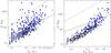 |
Fig. 4 Mass-size plots for clumps extracted with Gaussclumps (left panel) and Clumpfind (right panel) for all clumps in our IRDCs. The solid lines represent the empirical lower limit threshold for high-mass star formation |

Statistics of cross-identifications of Gaussclumps/Clumpfind sources with star formation signposts and clustering information.
4.5. Comments on individual IRDCs (based on Gaussclumps)
IRDC G329. The IRAS sources 15566-5304, 15579-5303, 15573-5307, and 15574-5306 are associated with clumps in the field of G329. The EGOs identified in this region were cataloged as “possible” massive young stellar object (MYSO) outflow candidates by Cyganowski et al. (2008). Masers (OH and CH3OH) toward a dozen of clumps were reported by Caswell et al. (1995).
IRDC G331. The source IRAS 16070−5107 is associated with a clump in the field of G331. One clump is associated with the radio continuum source G331.4+00.0, which was observed in an all-sky survey of HII regions at 4.85 GHz (Kuchar & Clark 1997). We retrieved C18O (1–0) data from the Three-mm Ultimate Mopra Milky way Survey (ThrUMMS6) and found that the emission in the lower left-hand corner in G331 (see Fig. 1), where the radio source is located, has a different systemic velocity (~−82 km s-1).
IRDC G335. Together with the IRDC G343, G335 has the highest number of clumps. Eight IRAS sources are associated with clumps in G335. We find two EGOs in this region: the first one, G335.43−0.24, was cataloged as a “possible” MYSO candidate and the second one, G335.06−0.43, as a “likely” MYSO outflow candidate (Cyganowski et al. 2008). The bubble S42 was identified by visual inspection of Spitzer/GLIMPSE images in Churchwell et al. (2006) and was cataloged as a “broken or incomplete” ring. The emission at 870 μm is tracing the eastern side of the dusty shell (see the bottom panel of Fig. 1).
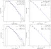 |
Fig. 5 Differential mass functions, dN/dM ∝ Mα, for clumps from Gaussclumps (upper panels) and clumps from Clumpfind (lower panels). The dashed blue lines represent fits to single power laws and the dot-dashed pink lines represent the fits to log-normal distributions. The parameters α, σ, and μ are given in each panel. The vertical dotted lines indicate the 6σrms (15 M⊙) mass given by the noisiest map. |
IRDC G337. One clump is associated with the source IRAS 16340-4732. The EGO G337.16−0.39 is found in this field and was cataloged a “likely” MYSO outflow candidate (Cyganowski et al. 2008). The Galactic radio source GRS 337.10−00.20, located northwest of the central filament, is probably not part of the IRDC complex because of different velocity components found for several line tracers. Previous studies of 337.10−00.20 show two velocity components in the H90α profile, at −73 km s-1 and at −59 km s-1 (Sarma et al. 1997), one velocity component at −73 km s-1 in the H190α profile (Wilson et al. 1970), and four velocity components in the CI profile, at 108, −75, −36, and −22 km s-1 (Huang et al. 1999). We confirm that this part of the field is at a different systemic velocity (~ − 72 km s-1) by retrieving N2H+ (1–0) data from the Millimeter Astronomy Legacy Team 90 GHz (MALT90) survey (Foster et al. 2011).
IRDC G343. The source IRAS 16575-4252 is associated with clumps in the field of G343. Three “possible” MYSO outflow candidates and one “likely” outflow candidate from Cyganowski et al. (2008) are associated with clumps in this region. No maser observations are reported in the literature.
IRDC G345. The three IRAS sources 17010-4124, 17014-4129, and 17018-4127 are associated with clumps in this field. Masers (OH, H2O, and CH3OH) were reported by Caswell et al. (1995) toward a couple of clumps. The EGOs G345.00-0.22a, G345.00-0.22b, and G345.13-0.17 were cataloged by Cyganowski et al. (2008) as “possible” MYSO outflow candidates. Fish et al. (2003) have found a distance of 2.9 kpc to one of the clumps associated with an IRAS source, which is actually a UC HII (Garay et al. 2006). Garay et al. (2007) carried out observations with the Swedish-ESO Submillimeter Telescope (SEST) at 1.2 mm toward the southern part of the filament that connects to the UC HII G345.001-0.22. The morphology at 1.2 mm is similar to that we see in the bottom panel in Fig. 2. These authors used a kinematic distance of 2.7 kpc. We use a distance of 2.8 kpc based on our N2H+ (3–2) line observations.
4.6. Mass-size relation for HMSF
Figure 4 shows the mass-size relationship for clumps extracted with Gaussclumps (left panel) and Clumpfind (right panel). We plot two HMSF lower thresholds: the one proposed by Krumholz & McKee (2008; hereafter KM08), who found a limit in NH2 = 2.13 × 1023 cm-2 (or 1 g cm-2) to avoid fragmentation and to allow high-mass stars to form, and the one discussed on empirical basis by Kauffmann & Pillai (2010; hereafter KP10). For the sake of comparison with those criteria, clump masses were computed again by decreasing the dust opacity values given in Ossenkopf & Henning (1994) by a factor of 1.5, as done in KP10. Additionally, we make a reduction of ln(2) ≈ 0.69 in the total mass to account for the mass contained in the half peak column density contour.
In Fig. 4, the percentage of clumps (found with Gaussclumps) that lie above the KP10 relation with and without association to star formation signpost is 19% and 9%, respectively, while 3% and <1% of clumps (with and without association to star formation signpost) satisfy the much more stringent threshold of KM08. The percentages of clumps (identified with Clumpfind) above the KP10 relation are 8% and 1% (with and without association to star formation signpost). All Clumpfind sources lie below the threshold of KM08.
4.7. Mass distribution of clumps in IRDCs
In Fig. 5, we present the differential mass functions for the 510 clumps extracted with Gaussclumps (upper panels) and the 352 sources from Clumpfind (lower panels). We plot the mass distribution using two approaches: in the first (left panels), the bin size was uniform with uncertainty given by a Poisson distribution. In the second (right panels), we followed the technique by Maíz Apellániz & Úbeda (2005) in which the bin size is variable so that the number of clumps per bin is approximately constant in order to minimize the binning biases. The uncertainty is derived from a binomial distribution according to Maíz Apellániz & Úbeda (2005).
In all cases we fit the differential mass distribution with a single power-law function  (4)where dN is the number of objects in dM, dM the mass bin, and α the power-law index. In addition, we fit a lognormal function:
 ![Mathematical equation: \begin{equation} \frac{{\rm d}N}{{\rm d}M} \propto \frac{1}{M\sigma}\exp\left[-\frac{(\ln M - \mu)^2}{2\sigma^2}\right], \label{Elognor} \end{equation}](/articles/aa/full_html/2014/01/aa22310-13/aa22310-13-eq99.png) (5)where σ is the dispersion and μ is related to the peak mass (Mpeak = eμ − σ2).
(5)where σ is the dispersion and μ is related to the peak mass (Mpeak = eμ − σ2).
In Fig. 5, we present the least-squares fits to single power laws, dN/dM ∝ Mα, with α = −1.62 ± 0.08 and αvar = −1.68 ± 0.10 for Gaussclumps (upper panels) with uniform and variable bin size, respectively, and to slopes α = −1.50 ± 0.09 and αvar = −1.59 ± 0.12 for Clumpfind (lower panels). In Fig. 5, we also present fits to log-normal distributions, with Mpeak = 0.61 ± 0.92 M⊙, σ = 1.78 ± 0.23 and Mpeak,var = 1.70 ± 1.76 M⊙, σvar = 1.59 ± 0.14 for Gaussclumps and Mpeak = 1.98 ± 2.64 M⊙, σ = 1.66 ± 0.18 and Mpeak,var = 2.91 ± 2.79 M⊙, σvar = 1.57 ± 0.12 for Clumpfind. The vertical dotted line indicates the 6σrms (15 M⊙) mass given by the noisiest map. As for the variable bin size, masses higher than 15 M⊙ were plotted and used in the fit. Since the fits to log-normal functions result in peak masses, Mpeak, below our 6σrms threshold of 15 M⊙, in what follows, we focus on the index obtained with the single power-law fits.
We find good agreement, within the uncertainties, between the mass distribution obtained with either Gaussclumps or Clumpfind. Moreover, these indices were similar when using a variable or uniform bin size. The single power-law index of our IRDC mass distribution has a mean and standard deviation of α = −1.60 and 0.06, respectively.
To check the effects in the mass distribution index due to different assumptions in, say, the source decomposition, estimation of masses, contribution of extended emission, and temperatures, we tested several scenarios with Clumpfind, using a 3σrms threshold and a 2σrms stepsize (see Appendix A for more details). The obtained indices have a mean and standard deviation of α = −1.68 and 0.15, respectively.
5. Discussion
5.1. Criteria for high-mass star formation
Less than 19% of the clumps found with Gaussclumps lie above the KM08 and KP10 thresholds. The majority of them have the mass needed to form high-mass stars, or they have already formed them. Clumps with no association to a star formation signpost are very interesting candidates for sources in the earliest phases of high-mass stellar cluster evolution. All clumps found with Clumpfind are located below the KM08 threshold. However, some of these clumps, as well as some found with Gaussclumps may contain higher surface density structures that are diluted within the beam. This can also explain the difference in percentage of clumps above both thresholds using different decomposition methods (see Fig. 4). As we found in Sect. 4.2, Gaussclumps tends to find more and smaller sources than does Clumpfind.
On the other hand, the eleven clumps observed in N2H+ (3−2) are all above the threshold discussed by KP10, while five of them lie above the KM08 one. Additionally, we can consider these clumps as dominated by gravity and either on the verge of collapse or already collapsing sources, according to their virial parameters.
5.2. Mass spectra
Making a comparison of the mass distribution indices is a hard task due to the many assumptions authors made when, extracting sources and estimating masses, etc. Several authors use extinction maps (Simon et al. 2006a; Marshall et al. 2009; Peretto & Fuller 2010; Ragan et al. 2009) while others make use of (sub)millimeter continuum maps (Rathborne et al. 2006; Miettinen 2012). In an attempt to compare our results with those of other authors, we fitted a single power law to our mass distribution using as many of their assumptions as possible: e.g., temperature, dust opacity, and threshold and stepsize (in the case of Clumpfind).
Figure 6 present the indices of the cloud/clump/core mass distribution for IRDCs and other HMSFRs from the literature. We plot those indices and compare them with our estimated values.
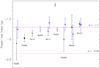 |
Fig. 6 Comparison of α values from the literature and our estimates. All symbols but six-pointed stars represent values obtained by other authors. Six-pointed star symbols represent our estimations taking different assumptions into account. Vertical lines represent the 1σ uncertainties. Horizontal lines show the index of the CO clump mass distribution (solid line) and the index of the IMF (broken line). References: Ra06 (Rathborne et al. 2006), Si06b (Simon et al. 2006b), Pe10 (Peretto & Fuller 2010), Ma09 (Marshall et al. 2009), Mi12 (Miettinen 2012), Ra09 (Ragan et al. 2009), Re06a (Reid & Wilson 2006a), Mo04 (Mookerjea et al. 2004), Mu07 (Muñoz et al. 2007). |
Marshall et al. (2009), Ragan et al. (2009), and Peretto & Fuller (2010) have studied the mass distribution of IRDCs obtained from extinction maps. In particular, Ragan et al. (2009) computed the mass distribution of cores using Clumpfind in 11 IRDCs and fitted broken power laws of αlow = −0.52 ± 0.04 and αhigh = −1.76 ± 0.05 for masses lower than 40 M⊙ and for masses greater than 40 M⊙, respectively. Using Gaussclumps, the slope becomes shallower: αhigh = −1.15 ± 0.04 and αlow = −0.64 ± 0.07 for the same break-point mass. We plot in Fig. 6αhigh for both Gaussclumps and Clumpfind since they are not consistent with each other within the uncertainties. Peretto & Fuller (2010) find that a lognormal distribution better fitted the mass distribution of “fragments” with masses higher than 10 M⊙. They also obtained the index for clouds, α = −1.85 ± 0.07. Marshall et al. (2009) found a similar α = −1.75 ± 0.06 for Mclouds > 1.7 × 10³ M⊙.
Using 13CO observations, Simon et al. (2006b) find a mass distribution of α = −1.97 ± 0.09 for IRDCs. This slope results from a fit to the high-mass end of the molecular cloud distribution (for Mclouds > 103.5 M⊙).
We computed our α value again to compare it with the α = −2.1 ± 0.4 estimated by Rathborne et al. (2006) for cores within IRDCs. They extracted core properties from the 1.2 mm dust continuum emission. We fitted the mass distribution including clumps with no signposts of star formation (extracted with Gaussclumps) and used a temperature of 15 K. We obtained α = −1.75 ± 0.21. As we can see in Fig. 6, their result is consistent with our estimate, but it is also consistent, within their uncertainties, with the stellar IMF (α = −2.35).
Miettinen (2012) mapped four IRDCs with the LABOCA instrument and obtained α = −1.8 ± 0.1 for clump masses above 1500 M⊙. We ran Clumpfind using a 3σrms threshold and a 3σrms stepsize and used three temperatures: 15 K for the clumps with no signpost of star formation, 30 K for HII regions and IRAS sources, and 20 K for the rest of the clumps. The bin size was Δlog (M/M⊙) ≈ 0.44. With these assumptions, we obtained α = −1.59 ± 0.14.
Mookerjea et al. (2004) studied the giant molecular cloud RCW 106 at 1.2 mm and found indices of α = −1.5 ± 0.3 (using Gaussclumps) and α = −1.7 ± 0.3 (with Clumpfind) after decomposing the dust emission into clumps. Since their values using two algorithms are consistent with each other, in Fig. 6, we plot the value for Clumpfind. In this case, our estimation of α = −1.87 ± 0.22 was obtained by assuming two different temperatures: 20 K for the clumps with no signposts of star formation and 40 K for the rest.
The mass distribution of the HMSFR NGC 6334 has been found to be similar to the CO mass distribution with α = −1.62 ± 0.07, from observations at 1.2 mm (Muñoz et al. 2007). We ran Clumpfind using a threshold of 3σrms, a stepsize of 2σrms, and a single temperature of 17 K. By making those assumptions, we obtain α = −1.64 ± 0.16.
Reid & Wilson (2005, 2006a) decomposed emission of (sub)mm maps (at 450 μm and 850 μm) of the HMSFRs NGC 7538 and M17 with Clumpfind. Broken power laws were fitted to their differential mass functions at 870 μm with indices at the high-mass end of αhigh = −2.0 ± 0.3 for NGC 7538 and αhigh = −1.5 ± 0.1 for M17. In Fig. 6, we plot the value for NGC 7538. Our computation of the index assumes a 3σrms threshold and a 2σrms stepsize for Clumpfind, a temperature of 35 K, an opacity spectral index of β = 1.5, and κν = 0.87 cm2 gr-1. We then obtain α = −1.63 ± 0.15. It is important to point out that Reid & Wilson (2006b) carried out a study in which they found that the high-mass end of seven mass distributions, including those of NGC 7538 and M17, is αhigh = −2.4 ± 0.1, resembling that of the stellar IMF.
In addition, we used the flux densities from the ATLASGAL compact source catalog of Contreras et al. (2013) for five of our regions in order to fit the clump mass distribution. Assuming a single temperature of 18 K, we found α = −1.70 ± 0.30 (for clumps with Mclumps > 100 M⊙), which is consistent with the value obtained by us.
As we can see from this revision and from Fig. 6, our derived α’s, as well as most of those obtained by other authors, are consistent with each other within the uncertainties and with the CO clump mass distribution.
6. Summary
We mapped the 870 μm dust continuum emission of six IRDCs with the LABOCA instrument and carried out molecular line observations of the N2H+ (3–2) line with the APEX2A receiver both with the APEX telescope. Our main results can be summarized as follows:
-
We estimated (“near”) kinematic distances of2.7–3.2 kpc using the N2H+ (3–2) line.
-
We obtained virial masses for 11 clumps. Their virial parameters indicate that these clumps are dominated by gravity, either on the verge of collapse or already collapsing.
-
Each IRDC was decomposed into clumps by using two automated algorithms, namely Gaussclumps and Clumpfind. The mean Reff is 0.20 pc for the Gaussclumps method, taking a total of 510 sources in account, while the Clumpfind mean Reff is 0.40 pc for 352 sources. The clump masses have been found in the range of 6 to 2692 M⊙ for Gaussclumps and 7 to 4254 M⊙ for Clumpfind.
-
The percentage of clumps that lie above the HMSF threshold discussed by Kauffmann & Pillai (2010) with and without association to star formation signpost is 19% and 9%, respectively, while 3% and <1% of clumps (with and without association to star formation signpost) satisfy the much more stringent threshold of Krumholz & McKee (2008). The percentages of clumps (identified with Clumpfind) above the KP10 relation are 8% and 1% (with and without association to star formation signpost). All Clumpfind sources lie below the threshold of KM08.
-
Using two methods of binning, the mass distribution of the decomposed emission into clumps has been fitted with a power law whose index is α = −1.60 ± 0.06. This index is consistent with the CO clump mass distribution and other HMSFRs.
Rest frequencies and upper level energies from the CDMS as of February 2011.
Main-beam and forward efficiencies are from http://www.apex-telescope.org/telescope/efficiency/index.php
Acknowledgments
L.G. acknowledges support for this research from the International Max Planck Research School (IMPRS) for Astronomy and Astrophysics at the Universities of Bonn and Cologne, CONICYT (Chile) through project BASAL PFB-06, and CSIRO Astronomy and Space Science. L.G. would like to thank A. Belloche for his help with the use of Gaussclumps. J.B.P. thanks financial support from UNAM-PAPIIT grant number IN103012. We thank the referee for providing helpful comments and suggestions. This work was partially funded by the ERC Advanced Investigator Grant GLOSTAR (247078). This work is based in part on observations made with the Spitzer Space Telescope, which is operated by the Jet Propulsion Laboratory, California Institute of Technology, under a contract with NASA. This research made use of SIMBAD database, operated at the CDS, Strasbourg, France.
References
- Bastian, N., Covey, K. R., & Meyer, M. R. 2010, ARA&A, 48, 339 [NASA ADS] [CrossRef] [Google Scholar]
- Battersby, C., Bally, J., Jackson, J. M., et al. 2010, ApJ, 721, 222 [NASA ADS] [CrossRef] [Google Scholar]
- Belloche, A., Schuller, F., Parise, B., et al. 2011, A&A, 527, A145 [NASA ADS] [CrossRef] [EDP Sciences] [Google Scholar]
- Bertoldi, F., & McKee, C. F. 1992, ApJ, 395, 140 [NASA ADS] [CrossRef] [Google Scholar]
- Blitz, L. 1993, in Protostars and Planets III, eds. E. H. Levy, & J. I. Lunine, 125 [Google Scholar]
- Carey, S. J., Noriega-Crespo, A., Mizuno, D. R., et al. 2009, PASP, 121, 76 [NASA ADS] [CrossRef] [Google Scholar]
- Caswell, J. L., Vaile, R. A., & Forster, J. R. 1995, MNRAS, 277, 210 [NASA ADS] [Google Scholar]
- Churchwell, E., Povich, M. S., Allen, D., et al. 2006, ApJ, 649, 759 [NASA ADS] [CrossRef] [Google Scholar]
- Contreras, Y., Schuller, F., Urquhart, J. S., et al. 2013, A&A, 549, A45 [NASA ADS] [CrossRef] [EDP Sciences] [Google Scholar]
- Cyganowski, C. J., Whitney, B. A., Holden, E., et al. 2008, AJ, 136, 2391 [NASA ADS] [CrossRef] [Google Scholar]
- Elmegreen, B. G., & Efremov, Y. N. 1997, ApJ, 480, 235 [NASA ADS] [CrossRef] [Google Scholar]
- Fich, M., Blitz, L., & Stark, A. A. 1989, ApJ, 342, 272 [NASA ADS] [CrossRef] [Google Scholar]
- Fish, V. L., Reid, M. J., Wilner, D. J., & Churchwell, E. 2003, ApJ, 587, 701 [NASA ADS] [CrossRef] [Google Scholar]
- Foster, J. B., Jackson, J. M., Barnes, P. J., et al. 2011, ApJS, 197, 25 [NASA ADS] [CrossRef] [Google Scholar]
- Garay, G., Brooks, K. J., Mardones, D., & Norris, R. P. 2006, ApJ, 651, 914 [NASA ADS] [CrossRef] [Google Scholar]
- Garay, G., Mardones, D., Brooks, K. J., Videla, L., & Contreras, Y. 2007, ApJ, 666, 309 [NASA ADS] [CrossRef] [Google Scholar]
- Güsten, R., Nyman, L. Å., Schilke, P., et al. 2006, A&A, 454, L13 [NASA ADS] [CrossRef] [EDP Sciences] [Google Scholar]
- Hildebrand, R. H. 1983, QJRAS, 24, 267 [NASA ADS] [Google Scholar]
- Hsu, W.-H., Hartmann, L., Heitsch, F., & Gómez, G. C. 2010, ApJ, 721, 1531 [NASA ADS] [CrossRef] [Google Scholar]
- Huang, M., Bania, T. M., Bolatto, A., et al. 1999, ApJ, 517, 282 [NASA ADS] [CrossRef] [Google Scholar]
- Kauffmann, J., & Pillai, T. 2010, ApJ, 723, L7 [NASA ADS] [CrossRef] [Google Scholar]
- Kauffmann, J., Bertoldi, F., Bourke, T. L., Evans, II, N. J., & Lee, C. W. 2008, A&A, 487, 993 [NASA ADS] [CrossRef] [EDP Sciences] [Google Scholar]
- Klein, B., Philipp, S. D., Krämer, I., et al. 2006, A&A, 454, L29 [NASA ADS] [CrossRef] [EDP Sciences] [Google Scholar]
- Kramer, C., Stutzki, J., Rohrig, R., & Corneliussen, U. 1998, A&A, 329, 249 [NASA ADS] [Google Scholar]
- Krumholz, M. R., & McKee, C. F. 2008, Nature, 451, 1082 [NASA ADS] [CrossRef] [PubMed] [Google Scholar]
- Kuchar, T. A., & Clark, F. O. 1997, ApJ, 488, 224 [NASA ADS] [CrossRef] [Google Scholar]
- Lada, C. J., & Lada, E. A. 2003, ARA&A, 41, 57 [NASA ADS] [CrossRef] [Google Scholar]
- Lada, E. A., Bally, J., & Stark, A. A. 1991, ApJ, 368, 432 [NASA ADS] [CrossRef] [Google Scholar]
- López, C., Bronfman, L., Nyman, L.-Å., May, J., & Garay, G. 2011, A&A, 534, A131 [NASA ADS] [CrossRef] [EDP Sciences] [Google Scholar]
- MacLaren, I., Richardson, K. M., & Wolfendale, A. W. 1988, ApJ, 333, 821 [NASA ADS] [CrossRef] [Google Scholar]
- Maíz Apellániz, J., & Úbeda, L. 2005, ApJ, 629, 873 [NASA ADS] [CrossRef] [Google Scholar]
- Marshall, D. J., Joncas, G., & Jones, A. P. 2009, ApJ, 706, 727 [NASA ADS] [CrossRef] [Google Scholar]
- Mathis, J. S., Rumpl, W., & Nordsieck, K. H. 1977, ApJ, 217, 425 [NASA ADS] [CrossRef] [Google Scholar]
- Miettinen, O. 2012, A&A, 542, A101 [NASA ADS] [CrossRef] [EDP Sciences] [Google Scholar]
- Mookerjea, B., Kramer, C., Nielbock, M., & Nyman, L.-Å. 2004, A&A, 426, 119 [NASA ADS] [CrossRef] [EDP Sciences] [Google Scholar]
- Muñoz, D. J., Mardones, D., Garay, G., et al. 2007, ApJ, 668, 906 [NASA ADS] [CrossRef] [Google Scholar]
- Ossenkopf, V., & Henning, T. 1994, A&A, 291, 943 [NASA ADS] [Google Scholar]
- Peretto, N., & Fuller, G. A. 2010, ApJ, 723, 555 [NASA ADS] [CrossRef] [Google Scholar]
- Pillai, T., Wyrowski, F., Carey, S. J., & Menten, K. M. 2006, A&A, 450, 569 [NASA ADS] [CrossRef] [EDP Sciences] [Google Scholar]
- Pineda, J. E., Rosolowsky, E. W., & Goodman, A. A. 2009, ApJ, 699, L134 [NASA ADS] [CrossRef] [Google Scholar]
- Ragan, S. E., Bergin, E. A., & Gutermuth, R. A. 2009, ApJ, 698, 324 [NASA ADS] [CrossRef] [Google Scholar]
- Rathborne, J. M., Jackson, J. M., & Simon, R. 2006, ApJ, 641, 389 [NASA ADS] [CrossRef] [Google Scholar]
- Rathborne, J. M., Jackson, J. M., Chambers, E. T., et al. 2010, ApJ, 715, 310 [NASA ADS] [CrossRef] [Google Scholar]
- Reid, M. A., & Wilson, C. D. 2005, ApJ, 625, 891 [NASA ADS] [CrossRef] [Google Scholar]
- Reid, M. A., & Wilson, C. D. 2006a, ApJ, 644, 990 [NASA ADS] [CrossRef] [Google Scholar]
- Reid, M. A., & Wilson, C. D. 2006b, ApJ, 650, 970 [NASA ADS] [CrossRef] [Google Scholar]
- Risacher, C., Vassilev, V., Monje, R., et al. 2006, A&A, 454, L17 [NASA ADS] [CrossRef] [EDP Sciences] [Google Scholar]
- Salpeter, E. E. 1955, ApJ, 121, 161 [Google Scholar]
- Sarma, A. P., Goss, W. M., Green, A. J., & Frail, D. A. 1997, ApJ, 483, 335 [NASA ADS] [CrossRef] [Google Scholar]
- Schuller, F. 2012, in SPIE Conf. Ser., 8452 [Google Scholar]
- Schuller, F., Menten, K. M., Contreras, Y., et al. 2009, A&A, 504, 415 [NASA ADS] [CrossRef] [EDP Sciences] [Google Scholar]
- Simon, R., Jackson, J. M., Rathborne, J. M., & Chambers, E. T. 2006a, ApJ, 639, 227 [NASA ADS] [CrossRef] [Google Scholar]
- Simon, R., Rathborne, J. M., Shah, R. Y., Jackson, J. M., & Chambers, E. T. 2006b, ApJ, 653, 1325 [NASA ADS] [CrossRef] [Google Scholar]
- Siringo, G., Kreysa, E., Kovács, A., et al. 2009, A&A, 497, 945 [NASA ADS] [CrossRef] [EDP Sciences] [Google Scholar]
- Stutzki, J., & Guesten, R. 1990, ApJ, 356, 513 [NASA ADS] [CrossRef] [Google Scholar]
- Weidner, C., Kroupa, P., & Bonnell, I. A. D. 2010, MNRAS, 401, 275 [NASA ADS] [CrossRef] [Google Scholar]
- Williams, J. P., de Geus, E. J., & Blitz, L. 1994, ApJ, 428, 693 [NASA ADS] [CrossRef] [Google Scholar]
- Wilson, T. L., Mezger, P. G., Gardner, F. F., & Milne, D. K. 1970, A&A, 6, 364 [NASA ADS] [Google Scholar]
Appendix A: Tests using Clumpfind
Pineda et al. (2009) point out several weaknesses in the Clumpfind algorithm for estimating the mass distribution index when choosing the threshold and stepsize parameters. To check potential assumptions that can affect the estimation of the clump mass distribution index, we run Clumpfind for four different thresholds (2, 3, 4, and 7σrms) and nine stepsizes (from 2–10σrms in steps of 1σrms). As found in Pineda et al. (2009), the effect of increasing the threshold is that of decreasing the number of extracted clumps.
In the left-hand panel of Fig. A.1, we plot the power-law index (α) as a function of stepsize. Same symbols represent runs for a given threshold, i.e., crosses, squares, stars, and diamonds represent 2, 3, 4, and 7σ thresholds, respectively. The values of α are estimated for a single temperature (T = 18 K). We see that as the threshold and the stepsize increase, the mass distribution becomes shallower.
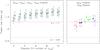 |
Fig. A.1 Clump mass distribution indices derived from Clumpfind runs for four different thresholds (2, 3, 4, and 7σrms) and nine stepsizes (2−10σrms), assuming one temperature of T = 18 K (left) and for a given threshold (3σrms) and stepsize (2σrms) making different assumptions as mentioned in Appendix A (right). |
Other tests for a given threshold (3σrms) and stepsize (2σrms) are plotted in the right-hand panel in Fig. 6:
-
Red triangles: we removed extended emission from each map by using the median filtering technique that calculates the median within a box of a given size. We used a box of about ten beams per side. Median maps were subtracted from the original maps. We then extracted clumps from these maps and estimated the indices by assuming one temperature (T = 18 K) for one case and two temperatures (18 K and 30 K) for the other.
-
Black circles: we artificially added 1σrms noise to each map, then extracted the clumps, and used one temperature (T = 18 K) for one case and two temperatures (18 K and 30 K) in the other.
-
Green squares: they correspond to the values we present in Fig. 5, which includes two values using the Gaussclumps algorithm.
-
Black diamond: we obtained this value assuming two temperatures (18 K and 30 K), and it does not include the clumps that might lie at very different distances (see Sect. 4.5). The number of clumps lying at different distance would corresponds to less than 4%.
-
Blue asterisk: the same as above but for clumps that do not have the signposts of star formation.
All Tables
Statistics of cross-identifications of Gaussclumps/Clumpfind sources with star formation signposts and clustering information.
All Figures
|
Fig. 1 Contour maps obtained with LABOCA at 870 μm overlaid on the Spitzer/MIPSGAL 24 μm images for the IRDCs G329 (top), G331 (middle), and G335 (bottom). The beam HPBW (21 |
| In the text | |
|
Fig. 2 Same as Fig. 1 but for the IRDCs G337 (top), G343 (middle), and G345 (bottom). Contours for G337 are 3, 6, 12, 24, 48, 96, 192 times 0.031 Jy beam-1, the rms noise of the image. Contours for G343 are 3, 6, 12, 24, 48, 96 times 0.028 Jy beam-1, the rms noise of the image. Contours for G345 are 3, 6, 12, 24, 48, 96, 192, 384 times 0.037 Jy beam-1, the rms noise of the image. |
| In the text | |
|
Fig. 3 APEX2A spectra (histograms) of the N2H+ (3–2) line. The red solid lines indicate the relative intensities for each of the 29 hyperfine components. P labels refer to the positions marked in Figs. 1 and 2 with red stars. |
| In the text | |
|
Fig. 4 Mass-size plots for clumps extracted with Gaussclumps (left panel) and Clumpfind (right panel) for all clumps in our IRDCs. The solid lines represent the empirical lower limit threshold for high-mass star formation |
| In the text | |
|
Fig. 5 Differential mass functions, dN/dM ∝ Mα, for clumps from Gaussclumps (upper panels) and clumps from Clumpfind (lower panels). The dashed blue lines represent fits to single power laws and the dot-dashed pink lines represent the fits to log-normal distributions. The parameters α, σ, and μ are given in each panel. The vertical dotted lines indicate the 6σrms (15 M⊙) mass given by the noisiest map. |
| In the text | |
|
Fig. 6 Comparison of α values from the literature and our estimates. All symbols but six-pointed stars represent values obtained by other authors. Six-pointed star symbols represent our estimations taking different assumptions into account. Vertical lines represent the 1σ uncertainties. Horizontal lines show the index of the CO clump mass distribution (solid line) and the index of the IMF (broken line). References: Ra06 (Rathborne et al. 2006), Si06b (Simon et al. 2006b), Pe10 (Peretto & Fuller 2010), Ma09 (Marshall et al. 2009), Mi12 (Miettinen 2012), Ra09 (Ragan et al. 2009), Re06a (Reid & Wilson 2006a), Mo04 (Mookerjea et al. 2004), Mu07 (Muñoz et al. 2007). |
| In the text | |
|
Fig. A.1 Clump mass distribution indices derived from Clumpfind runs for four different thresholds (2, 3, 4, and 7σrms) and nine stepsizes (2−10σrms), assuming one temperature of T = 18 K (left) and for a given threshold (3σrms) and stepsize (2σrms) making different assumptions as mentioned in Appendix A (right). |
| In the text | |
Current usage metrics show cumulative count of Article Views (full-text article views including HTML views, PDF and ePub downloads, according to the available data) and Abstracts Views on Vision4Press platform.
Data correspond to usage on the plateform after 2015. The current usage metrics is available 48-96 hours after online publication and is updated daily on week days.
Initial download of the metrics may take a while.