| Issue |
A&A
Volume 561, January 2014
|
|
|---|---|---|
| Article Number | A46 | |
| Number of page(s) | 8 | |
| Section | Stellar atmospheres | |
| DOI | https://doi.org/10.1051/0004-6361/201321977 | |
| Published online | 23 December 2013 | |
The close environment of high-mass X-ray binaries at high angular resolution
I. VLTI/AMBER and VLTI/PIONIER near-infrared interferometric observations of Vela X-1⋆
1 LESIA, Observatoire de Paris, CNRS UMR 8109, UPMC, Université Paris-Diderot, Paris Sciences et Lettres, 5 place Jules Janssen, 92195 Meudon, France
e-mail: choquet@stsci.edu
2 Space Telescope Science Institute, 3700 San Martin Drive, Baltimore MD-21218, USA
3 UJF-Grenoble 1/CNRS-INSU, Institut de Planétologie et d’Astrophysique de Grenoble (IPAG) UMR 5274, 38041 Grenoble, France
4 European Southern Observatory, Alonzo de Córdova 3107, 19001 Casilla, Santiago 19, Chile
5 Instituto de Astronomia, Geofìsica e Ciências Atmosféricas, Universidade de São Paulo, Rua do Matão 1226, Cidade Universitária, SP 05508-900 São Paulo, Brazil
6 Max-Planck-Institut für Astronomie, Königstuhl 1, 69117 Heidelberg, Germany
Received: 28 May 2013
Accepted: 4 November 2013
Context. Recent improvements in the sensitivity and spectral resolution of X-ray observations have led to a better understanding of the properties of matter in the near vicinity of high-mass X-ray binaries (HMXB) hosting a supergiant star and a compact object. However, the geometry and physical properties of their environments on larger scales (up to a few stellar radii) are currently only predicted by simulations but have never been directly observed.
Aims. We aim to explore the environment of Vela X-1 at a few stellar radii (R⋆) of the supergiant using spatially resolved observations in the near-infrared, and to study its dynamical evolution along the nine-day orbital period of the system.
Methods. We observed Vela X-1 in 2010 and 2012 using near-infrared long baseline interferometry at the Very Large Telescope Interferometer (VLTI), respectively with the AMBER instrument in the K band (medium spectral resolution), and the PIONIER instrument in the H band (low spectral resolution). The PIONIER observations span one orbital period to monitor possible evolutions in the geometry of the system.
Results. We resolved a structure of 8 ± 3 R⋆ from the AMBER K-band observations, and 2.0-1.2+0.7R* from the PIONIER H-band data. From the closure phase observable, we found that the circumstellar environment of Vela X-1 is symmetrical in the near-infrared. We observed comparable interferometric measurements between the continuum and the spectral lines in the K band, meaning that both emissions originate from the same forming region. From the monitoring of the system over one period in the H band in 2012, we found the signal to be constant with the orbital phase within the error bars.
Conclusions. We propose three possible scenarios for this discrepancy between the two measurements: 1) there is a strong temperature gradient in the supergiant wind, leading to a hot component that is much more compact than the cool part of the wind observed in the K band; 2) we observed a diffuse shell in 2010, possibly triggered by an off-state in the accretion rate of the neutron star that was dissolved in the interstellar medium in 2012 during our second observations; or 3) the structure observed in the H band was the stellar photosphere instead of the supergiant wind.
Key words: techniques: interferometric / circumstellar matter / stars: individual: Vela X-1
© ESO, 2013
1. Introduction
Supergiant high-mass X-ray binaries (Sg-HMXB) are binary systems hosting a compact stellar remnant (a black hole or neutron star) and a massive optical counterpart, usually an OB type supergiant of emitting a strong stellar wind. These systems have very high X-ray luminosities owing to accretion of matter from the massive companion by the compact object that is deeply embedded in the supergiant wind in a very energy-efficient process (see the review by Chaty 2011). They are intensively observed in high-energy spectral domains in order to better understand the processes at stake in accretion onto compact objects. In addition, because the X-ray luminosity is mostly related to the mass accretion rate in these systems, the compact object can be seen as a local probe of the density of matter evolving in the supergiant environment. This way, the clumpy nature of the wind of early-type supergiants has been analyzed and characterized by monitoring the variations in X-ray luminosity of Sg-HMXBs (Walter & Zurita Heras 2007). However, the way the compact object shapes this environment on a larger scale (up to a few tens of stellar radii) is still debated. Several numerical simulations have been carried out, implementing different forces with varying intensities (depending on the physical and geometric properties of the systems). Some simulations predict that the supergiant wind could be focused by the gravitational field of the compact object and form a gaseous tail in its wake (Hadrava & Čechura 2012). Other simulations show that the velocity of the line-driven wind could be inhibited or even propelled back toward the supergiant by the X-ray heating and photoionization of the compact object, in case of close proximity in the binary system (Hadrava & Čechura 2012; Krtička et al. 2012). Finally, recent simulations have revealed that in case of binary systems hosting a non-accreting pulsar, the colliding winds from both objects create shocked structures at 5 to 10 angular separations away from the stars (Bosch-Ramon et al. 2012).
To the best of our knowledge, these predicted structures in the environments of Sg-HMXBs have never been observed. These systems are usually at distances of a few kilo-parsec, with a typical size of a few tens of solar radii, making them very small targets with angular diameters on the order of a milli-arcsecond (mas). Only interferometric observations using baselines hundreds of meters long can spatially resolve the environment of these systems. We therefore carried out a pilot study on Vela X-1, using the Very Large Telescope Interferometer (VLTI) in the near-infrared.
Vela X-1 is one of the most studied Sg-HMXB. The system is located at a distance of d = 1.9 kpc from the Earth (Sadakane et al. 1985) and hosts a massive pulsar (identified as 4U 0900-40) and a B0.5I supergiant (identified as HD 77 581 or GP Vel) emitting a strong stellar wind. The mass and radius of the optical counterpart are estimated to be, respectively, M⋆ ~ 32 M⊙ and R⋆ ~ 24 R⊙ (Rawls et al. 2011). Its wind has a terminal velocity of V ~ 1105 km s-1 (Prinja et al. 1990) and a mass loss rate of Ṁ⋆ ~ 1.5 × 10⁻⁶ M⊙ yr-1 (Watanabe et al. 2006). The pulsar has a spin period of 283 s (McClintock et al. 1976). Its mass MX ~ 1.8 M⊙ is known to be one of the largest for a neutron star, and is regularly measured and refined through various methods (Barziv et al. 2001; Quaintrell et al. 2003; Rawls et al. 2011; Koenigsberger et al. 2012). Its mass lies at the limit predicted by several theories on the still unknown state of matter in neutron stars, and the precise estimation of the mass of the pulsar in Vela X-1 can put constraints that can rule out some of these theories. The pulsar is deeply embedded in the supergiant wind. It follows an eclipsing orbit with a period P of ~9 days (Kreykenbohm et al. 2008) and a projected semi-major axis a sin i ~ 49 R⊙ (Rawls et al. 2011), i.e., ~ 2 R⋆. Accretion from this wind is the main source of X-ray emission in this system, with a luminosity of LX ~ 3.5 × 1036 erg s-1 (Watanabe et al. 2006).
From X-ray monitoring of the system luminosity, it seems that the pulsar evolves in a highly clumpy stellar wind, whose inhomogeneities in the density of matter produce important and irregular flares and off-states in X-rays (Kreykenbohm et al. 2008; Fürst et al. 2010; Doroshenko et al. 2011). As is usual for Sg-HMXBs, the characteristics of the environment on a larger scale are not clearly understood, and have not been directly observed up to now. The presence of a trailing wake behind the pulsar has been suggested by UV (Sadakane et al. 1985) and X-ray (Watanabe et al. 2006) spectroscopic observations of Vela X-1. In addition, the latter authors demonstrated that the supergiant dynamics is affected by the X-ray photoionization of the wind between the star and the pulsar, leading to a reduction of the velocity of the line-driven wind. This analysis has been recently confirmed through numerical simulations by Krtička et al. (2012).
In order to spatially resolve the environment of Vela X-1 at a few stellar radii from the supergiant, we observed the system using near-infrared long baseline interferometry. We obtained two observations at VLTI in March 2010 and March 2012, with two different instruments, AMBER (Astronomical Multi-BEam combineR) in the K band and PIONIER (Precision Integrated-Optics Near-infrared Imaging ExpeRiment) in the H band. In Sect. 2 we describe the observations and instrumental setup. The data are analyzed in Sect. 3, and we discuss the results from the two data sets in Sect. 4. Our conclusions are summarized in Sect. 5.
2. Observations and data reduction
2.1. Instrument setup
Some useful characteristics of Vela X-1 are given in Table 1. We obtained data at two different epochs on Vela X-1, using two different infrared beam combiners at VLTI with two different sets of telescopes, in two different spectral bands. The first dataset was obtained in March 2010 with the AMBER instrument using the K spectral band (1.92−2.26 μm). The second dataset consists of four half nights spanning one orbital period of Vela X-1 in March 2012, and was acquired with the PIONIER instrument in the H band (1.5−1.8 μm). Overviews of the observations and of the telescope configurations are presented in Tables 3 and 2, respectively, with the corresponding orbital phase of Vela X-1. The orbital phase is computed using the ephemeris of Kreykenbohm et al. (2008), with the X-ray mid-eclipse time as a reference for the 0-phase.
Telescope configurations.
Overview of the observations.
2.1.1. AMBER observations
AMBER is a three-telescope spectro-interferometer at VLTI, working in the J, H, and K spectral bands (from 1 to 2.4 μm), and providing three different spectral resolutions (R ~ 30, R ~ 1500, and R ~ 12 000) (Petrov et al. 2007). The beams are spatially filtered using single-mode fibers to provide high-precision interferometric measurements (Coudé du Foresto 1998). The interference pattern is acquired using a multi-axial combination with non-redundant spatial coding, simultaneously with a photometric channel for each beam so as to calibrate the coherent flux.
The AMBER observations of Vela X-1 were carried out using three 8 m unit telescopes (UTs) at VLTI (UT1, UT3, and UT4), with baseline lengths ranging from 63 m to 130 m, using the K-band medium-resolution configuration of the instrument (R ~ 1500). The (u, v) coverage obtained for this observation is presented in Fig. 1. The FINITO (Fringe-Tracking Instrument of NIce and TOrino) fringe tracker (Le Bouquin et al. 2008) was used for these observations to stabilize the fringes and improve the precision of the interferometric measurements.
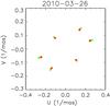 |
Fig. 1 Spatial frequencies of Vela X-1 covered during the AMBER observations. The color of the symbol ranges with the wavelength of the observations, from blue for the shortest wavelength (2.03 μm) to red for the longest (2.26 μm). |
2.1.2. PIONIER observations
PIONIER is a VLTI visitor instrument enabling the combination of four telescopes in the H band (Le Bouquin et al. 2011). Each observation thus simultaneously provides six visibility and three independent closure phase measurements at different spatial frequencies, which enables the observer to constrain the spatial intensity distribution of the observed target. To achieve high-precision interferometric measurements, the beams are spatially filtered using single-mode fibers, and combined using an integrated optics component (Benisty et al. 2009). Three different spectral resolutions can be used: broadband, R ~ 15, and R ~ 35.
The PIONIER observations of Vela X-1 were carried out using the four relocatable 1.8 m auxiliary telescopes (ATs) at VLTI, on stations A1, G1, I1, K0, providing baseline lengths ranging from 47 m to 129 m. Depending on the atmospheric conditions, either the broadband or the low-resolution modes (R ~ 15) were used. The log of the observations is presented in Table 4. The spatial frequencies covered by these observations are presented in Fig. 2.
Log of the PIONIER observations.
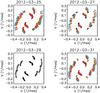 |
Fig. 2 Spatial frequencies of Vela X-1 covered during the PIONIER observations, for each night. Black symbols stands for broadband measurements, and colored symbols stand for low spectral resolution measurements (red, green, and blue correspond to measurements at, respectively, 1.59 μm, 1.68 μm, and 1.76 μm). |
2.2. Data reduction
The calibrated interferometric measurements were obtained using the AMBER data reduction software amdlib package (version 3.05; Tatulli et al. 2007; Chelli et al. 2009) for the AMBER observations, and with the PIONIER data reduction software pndrs1 (version 2.42; Le Bouquin et al. 2011) for the PIONIER observations. The stars used to calibrate the photometric and interferometric measurements are listed in Table 5.
The wavelength calibration of the AMBER data was obtained by fitting a part of the calibrated spectrum of Vela X-1 rich in telluric features with a model synthesized from spectroscopic parameters of atmospheric molecules using the high-resolution transmission molecular absorption database (HITRAN), water vapor and atmospheric models, and optical fiber dispersion (Mérand et al. 2010). For the AMBER analysis, measurements acquired at wavelengths lower than 2.03 μm are systematically discarded, since their quality is significantly worse than for longer wavelengths because of strong atmospheric absorption.
The spectral calibration of the PIONIER data was obtained with the PIONIER data reduction software, as described in Le Bouquin et al. (2011). The authors estimate the accuracy of the calibrated effective wavelengths to be 2%, which is sufficient for our analysis considering the 10% maximum resolution of our observations.
Calibrators used to reduce the interferometric data.
3. Results
3.1. AMBER spectroscopic analysis
We analyzed the spectrum of Vela X-1 obtained with AMBER and compared it to the 2 μm OB star atlas from Hanson et al. (1996). Four spectral lines are clearly observed, with signals of 4, 5, 3, and 2σ. They are referenced as three He I transitions (at wavelengths 2.058, 2.113, and 2.162 μm) and the hydrogen Brackett-γ (Br-γ) line at 2.166 μm. These recombination lines of helium and hydrogen are typical signatures of out-flowing gas close to OB supergiants (Najarro et al. 1994). The continuum emission can be related to the supergiant photosphere and to the free-free and free-bound emissions in the wind.
As a qualitative comparison with the spectra of B0.5 supergiants described in Hanson et al. (1996), Vela X-1 shows similar spectral features as a B0.5 Ib star, with the same lines in emission and absorptions. This is consistent with previous classifications of Vela X-1, which is described as a B0.5 Ia (Prinja & Massa 2010), a B0.5 Iae (Krtička et al. 2012), or a B0.5 Ib supergiant (Dupree et al. 1980) in the literature.
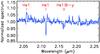 |
Fig. 3 Calibrated spectrum of Vela X-1 measured with AMBER. The error bars are about the size of the line (typically 2%). The positions of the four identified spectral features are marked by solid red lines. The dashed black line denotes the normalized value of the spectrum. |
3.2. AMBER interferometric analysis
The calibrated squared visibilities and closure phases measured with AMBER are presented respectively in Figs. 4 and 5.
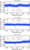 |
Fig. 4 Calibrated squared visibilities of Vela X-1 obtained with AMBER on the three baselines. The dashed horizontal red lines mark the values in the continuum, and the solid vertical red lines mark the identified spectral features. A dashed black line marks the squared visibility of an unresolved target. |
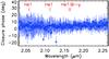 |
Fig. 5 Calibrated closure phases of Vela X-1 obtained with AMBER. The dashed red line marks the closure phase value in the continuum, and the solid vertical red lines mark the identified spectral features. |
3.2.1. Spectral analysis
We analyzed the interferometric observables of Vela X-1 measured at the wavelengths corresponding to the four spectral lines identified in Sect. 3.1, which are detailed in Table 6 (see also Figs. 4 and 5). Neither the squared visibilities nor the closure phase signal at these wavelengths are significantly different from the corresponding values in the continuum estimated from the mean visibilities over the spectral range: the differential signal between the continuum and the lines is at most 3% and 3°, respectively, for the squared visibilities and for the closure phase, but the statistical 1-sigma dispersions of the measurements over all the spectral channels are, respectively, 3–5% and 4°. As a consequence, this indicates that both the continuum and the lines have the same origin in the stellar wind, and are emitted within very similar formation regions.
3.2.2. Parametric modeling with the AMBER data
The values of the interferometric observables in the continuum detailed in Table 6 show that the system is partially resolved on the two longest baselines.We note that only one calibrator has been used for this observation, which can fail to remove some systematic errors in the science measurements. However, the calibrator HD 76304 has been carefully selected in the catalog from Mérand et al. (2005), dedicated to providing a reliable calibrator with precise angular diameter estimations for long-baseline optical interferometry. In addition, we checked that the piston levels between the acquisitions of Vela X-1 (35.7 μm rms) and of the calibrator (34.7 μm then 32.5 μm) are comparable and do not bias the calibration of the interferometric observables.
As the typical accuracy on the closure phase is 9° and includes possible systematic errors, the closure phase signal obtained with AMBER does not show any significant departure from the null value (see Fig. 5). As a consequence, we discarded it from the parametric modeling in order to reduce the number of degrees of freedom and improve the precision on the fit parameter. We then used the centro-symmetric model of a uniform disk, which produces a null closure phase signal before the first zero of the visibility function. The diameter of the disk is fitted to the measured squared visibilities. The error bar on the fitted diameter is computed with a variation of 1 from the minimum value of the reduced χ2, defined as 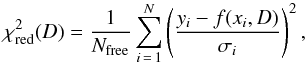 (1)with {yi} i ∈ [1,N] the measured squared visibilities, {σi} i ∈ [1,N] the corresponding uncertainties, {xi} i ∈ [1,N] the corresponding spatial frequencies, f the squared visibility function of a uniform disk, D the disk diameter, and Nfree the number of degrees of freedom.
We found a value of 1.27 ± 0.40 mas for the best-fit diameter of a uniform disk. The reduced χ2 as a function of the disk diameter is presented in Fig. 6. The squared visibilities of Vela X-1 measured with AMBER and computed with the best model are shown in Fig. 7. Assuming a distance of 1.9 kpc from the Earth (Sadakane et al. 1985), this corresponds to a disk radius of 8 ± 3 R⋆.
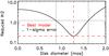 |
Fig. 6 Reduced χ2 between the AMBER data and a model of a uniform disk, as a function of the disk diameter. The 1-sigma error bars of the best diameter are computed by a variation of the reduced χ2 of one (dotted black lines) from the minimum (dashed red lines). |
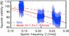 |
Fig. 7 Squared visibilities of Vela X-1 measured with AMBER (blue diamonds), and best model of a uniform disk with angular diameter of 1.27 ± 0.40 mas (solid red line, error bars in dashed red lines). |
3.3. PIONIER interferometric analysis
The calibrated squared visibilities and closure phases measured with PIONIER are presented respectively in Figs. 8 and 9.
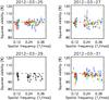 |
Fig. 8 Calibrated squared visibilities of Vela X-1 obtained with PIONIER for each observing night. Black symbols stand for broadband measurements, colored symbols for low spectral resolution measurements (blue at 1.59 μm, green at 1.68 μm, red at 1.76 μm). A dashed black line marks the squared visibility of an unresolved target. |
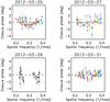 |
Fig. 9 Calibrated closure phases of Vela X-1 obtained with PIONIER. The colors are the same as in Fig. 8. A dashed black line marks the null closure phase of an unresolved target. |
3.3.1. Analysis over an orbital period
As a qualitative analysis, we compared the six squared visibilities and the four closure phases averaged over the half-nights for each observing night. The values are presented respectively in Figs. 10 and 11. We considered that their variation with the super-synthesis effect provided by Earth rotation along a night is not significant regarding the accuracy of the measurements. This is relevant since the dispersion of the data over a night is similar to their individual uncertainties.
We found that the variation of the interferometric signal over the four nights is marginally significant. The maximum variation is 6% and 1.5° respectively for the squared visibilities and the closure phases, which corresponds respectively to 2 and 1.6 times the typical spread of the data over a night. As a consequence, we conclude that the geometry and the symmetry of Vela X-1 slightly varied with the orbital phase during our observations. We do not further analyze these low signal-to-noise ratio signals for lack of data.
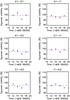 |
Fig. 10 Squared visibilities of Vela X-1 measured with PIONIER, averaged for each observing half-night. The error bars show the precision on the average. The dashed red lines mark the mean values over the four nights. |
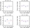 |
Fig. 11 Closure phases of Vela X-1 measured with PIONIER, averaged for each observing half-night. As in Fig. 10, the error bars show the precision on the mean of the data. The dashed red lines correspond to the mean values over the four observations. |
3.3.2. Parametric modeling with the PIONIER data
Considering the previous analysis, we adjusted the parametric model of a uniform disk to the entire set of the PIONIER data, regardless of the orbital phase of the system. As the closure phase signals do not show significant departures from the null value (see Fig. 11), we chose the centro-symmetric model of a uniform disk, and fit its diameter only to the squared visibility measurements. The precision on the best fit diameter is estimated with a variation of one of the reduced χ2 from the minimum value, as in Sect. 3.2.2.
The reduced χ2 curve is presented in Fig. 12, and the best fit is shown in Fig. 13. We found that the best model corresponds to a disk of diameter  mas, with asymmetric error bars. Assuming a distance of 1.9 kpc, this corresponds to a structure of radius
  .
.
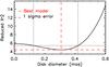 |
Fig. 12 Reduced χ2 between the squared visibilities measured with PIONIER and computed with a model of a uniform disk, as a function of the disk diameter. The 1-sigma error bars (dotted black lines) of the best diameter are computed by a variation of the reduced χ2 of one from the minimum value (dashed red lines). |
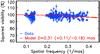 |
Fig. 13 All squared visibilities of Vela X-1 measured with PIONIER between March 25 and 31, 2012 (blue diamonds), and the best model of a uniform disk of diameter |

4. Discussion
During these two campaigns, we observed structures around Vela X-1 with significantly different sizes, of 8 ± 3 R⋆ and in 2010 and 2012, respectively. We discuss here several possible explanations for these different results.
Because the observations were carried out in different spectral bands, this difference in the measured diameters can be attributed to a thermal inhomogeneity in the wind. The temperature in hot supergiants varies typically from 10 000 K at 1−2 R⋆ to 5000 K at 5 R⋆ (Cidale 1998). The relation between the temperature law in the stellar wind and the size of the envelope observed in the H and K bands is, however, hard to predict without radiative transfer modeling, which is out of the scope of this study. We then compare our estimations to a basic temperature power law. Considering that the effective observing wavelength λmax reflects the maximum emission of a black body at temperature T, Wien’s law provides an estimation of the temperature of the observed material: 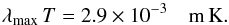 (2)Thus, our AMBER observations in the K and H bands can be related to parts of the wind at different temperatures, respectively, to a cooler part at 1350 K and a hotter part at 1720 K. Assuming that this temperature gradient can be described with a power law such that R ∝ Tα, our measurements lead to a power law with α = −6, which is significantly different from a black body at thermal equilibrium (R ∝ T-2, Stefan-Boltzmann law).
The second possible explanation for the discrepancy in the measured sizes is that we may have observed a diffuse gaseous shell around the system in 2010 that were no longer present during our observations in 2012. Assuming that the gas propagates at the terminal velocity of the wind, the lifetime of such a shell would be a few days. This envelope could be related to the accretion activity of Vela X-1, which is known to be highly variable from X-ray observations (Kreykenbohm et al. 2008; Fürst et al. 2010). The X-ray luminosity of the compact object irregularly turns off, leading to off-states lasting from a few seconds to one hour and during which the flux drops by a factor of ten or more. Analysis of these off-states by Doroshenko et al. (2011) demonstrates that they are due to a drop in the mass accretion rate of the pulsar (whose origin is still debated). Assuming a drop in the pulsar accretion rate of a factor of 20, we estimate the optical density of a shell at 8 R⋆ to be 1.3 times higher than the circumstellar matter at 2 R⋆ in a regular accretion state of the compact object. In addition, Bosch-Ramon et al. (2012) showed that in binary systems hosting a massive star and a non-accreting pulsar, the winds of both objects collide and produce a shocked flow extending up to a few times their angular separation, and spiraling with the orbital motion of the system. We might have witnessed a shocked structure of this nature in 2010, produced during an off-state of the pulsar, but spherical instead of spiraling, since seen edge-on.
The last possibility is that we observed two different components, i.e. the free-free emission of the stellar wind in the K-band observations, and the supergiant photosphere in the H-band observations. With an emission power spectrum decreasing with the shorter wavelength and a cut-off wavelength in the near-infrared at ≃3 μm, the free-free emission is smaller in the H band than in the K band, and the wind emission in the H band may be negligible compared to the supergiant photosphere. In addition, by extrapolation of the photosphere diameter of Rigel (B8Ia, 237 pc) measured by Aufdenberg et al. (2008), the photosphere of Vela X-1 should have a diameter of 0.34 mas, which corresponds to our PIONIER measurement. However, the size of the photosphere of Vela X-1 reported in the literature (Rawls et al. 2011; Quaintrell et al. 2003), corresponding to an angular diameter of 0.16 mas, was computed with higher precision from radial velocity measurements than from our measurements. As a consequence, we cannot safely state whether we observed the supergiant photosphere or the stellar wind close to supergiant with PIONIER observations.
5. Conclusion
We presented results of near-infrared interferometric observations of Vela X-1, carried out at VLTI at two different epochs (March 2010 and March 2012), and in two different spectral bands (respectively, in the K and H bands).
A centro-symmetric structure with a typical radius of 8 ± 3 stellar radii was resolved with the first instrumental setup at 2.2 μm. From the medium spectral resolution of the observations, we deduced that the system presents the same spectral features as a B0.5 Ib supergiant, and that the source of the four identified spectral lines is in the same formation region as the continuum. However, despite the better angular resolution provided by the second instrumental setup in the H band, no significant structure was observed in 2012, leading to a centro-symmetric structure of radius  stellar radii at 1.65 μm. This second set sampled the system orbital phase of Vela X-1 with four observations, but no significant variation was detected in the interferometric observables.
We discussed three possible explanations for this discrepancy in the diameter measurements:
-
The difference can come from a strong temperature gradient in thesupergiant wind, which could explain why the observed structurewas much more extended at 2.2 μm than at 1.65 μm.
-
We might have observed a diffuse gaseous shell in 2010 that could have dissolved into the interstellar medium in 2012. This structure could have been produced by an off-state in the accretion rate of the pulsar, shocked by the collision between the winds of the supergiant and of the pulsar.
-
We may have observed the supergiant photosphere instead of the stellar wind in our PIONIER observations.
To rule out one or the other scenario, further observations should be carried out simultaneously in both near-infrared spectral bands (H and K). In addition, simultaneous (or immediately before) observations in X-rays would provide information on the accretion activity of the pulsar, which could be related to the geometry of the stellar wind at a few stellar radii from the system. Depending on the results of these observations, radiative transfer modeling should be performed to better understand how the free-free emission scales in the wind of such a supergiant (as performed by Chesneau et al. 2010; Kaufer et al. 2012), and how the intensity distribution observed in 2010 is related to the shocked wind predicted by Bosch-Ramon et al. (2012).
Available at http://apps.jmmc.fr/~swmgr/pndrs
Software packages available at http://www.jmmc.fr
Acknowledgments
We are grateful to Olivier Chesneau for his helpful comments on the wind properties of B supergiants. This research has made use of CDS Astronomical Databases SIMBAD and VIZIER, of NASA’s Astrophysics Data System (ADS), of the Aspro and SearchCal services and of the AMBER data reduction package provided by the Jean-Marie Mariotti Center2. The research leading to these results has received funding from the European Community’s Seventh Framework Program under Grant Agreement 226604 (Fizeau exchange program).
References
- Aufdenberg, J. P., Ludwig, H.-G., Kervella, P., et al. 2008, in The Power of Optical/IR Interferometry: Recent Scientific Results and 2nd Generation, eds. A. Richichi, F. Delplancke, F. Paresce, & A. Chelli, 71 [Google Scholar]
- Barziv, O., Kaper, L., Van Kerkwijk, M. H., Telting, J. H., & Van Paradijs, J. 2001, A&A, 377, 925 [NASA ADS] [CrossRef] [EDP Sciences] [Google Scholar]
- Benisty, M., Berger, J.-P., Jocou, L., et al. 2009, A&A, 498, 601 [NASA ADS] [CrossRef] [EDP Sciences] [Google Scholar]
- Bildsten, L., Chakrabarty, D., Chiu, J., et al. 1997, ApJS, 113, 367 [NASA ADS] [CrossRef] [Google Scholar]
- Bosch-Ramon, V., Barkov, M. V., Khangulyan, D., & Perucho, M. 2012, A&A, 544, A59 [NASA ADS] [CrossRef] [EDP Sciences] [Google Scholar]
- Chaty, S. 2011, in Evolution of Compact Binaries, eds. L. Schmidtobreick, M. R. Schreiber, & C. Tappert, ASP Conf. Ser., 447, 29 [Google Scholar]
- Chelli, A., Utrera, O. H., & Duvert, G. 2009, A&A, 502, 705 [NASA ADS] [CrossRef] [EDP Sciences] [Google Scholar]
- Chesneau, O., Dessart, L., Mourard, D., et al. 2010, A&A, 521, A5 [NASA ADS] [CrossRef] [EDP Sciences] [Google Scholar]
- Cidale, L. S. 1998, ApJ, 502, 824 [NASA ADS] [CrossRef] [Google Scholar]
- Coudé du Foresto, V. 1998, in Fiber Optics in Astronomy III, eds. S. Arribas, E. Mediavilla, & F. Watson, ASP Conf. Ser., 152, 309 [Google Scholar]
- Doroshenko, V., Santangelo, A., & Suleimanov, V. 2011, A&A, 529, A52 [NASA ADS] [CrossRef] [EDP Sciences] [Google Scholar]
- Dupree, A. K., Gursky, H., Black, J. H., et al. 1980, ApJ, 238, 969 [NASA ADS] [CrossRef] [Google Scholar]
- Fürst, F., Kreykenbohm, I., Pottschmidt, K., et al. 2010, A&A, 519, A37 [NASA ADS] [CrossRef] [EDP Sciences] [Google Scholar]
- Hadrava, P., & Čechura, J. 2012, A&A, 542, A42 [NASA ADS] [CrossRef] [EDP Sciences] [Google Scholar]
- Hanson, M. M., Conti, P. S., & Rieke, M. J. 1996, ApJS, 107, 281 [Google Scholar]
- Kaufer, A., Chesneau, O., Stahl, O., et al. 2012, in ASP Conf. Ser. 464, eds. A. C. Carciofi, & T. Rivinius, 35 [Google Scholar]
- Koenigsberger, G., Moreno, E., & Harrington, D. M. 2012, A&A, 539, A84 [NASA ADS] [CrossRef] [EDP Sciences] [Google Scholar]
- Kreykenbohm, I., Wilms, J., Kretschmar, P., et al. 2008, A&A, 492, 511 [NASA ADS] [CrossRef] [EDP Sciences] [Google Scholar]
- Krtička, J., Kubát, J., & Skalický, J. 2012, ApJ, 757, 162 [NASA ADS] [CrossRef] [Google Scholar]
- Lafrasse, S., Mella, G., Bonneau, D., et al. 2010, VizieR Online Data Catalog, II/300 [Google Scholar]
- Le Bouquin, J.-B., Abuter, R., Bauvir, B., et al. 2008, Proc. SPIE, 7013, 701318 [CrossRef] [Google Scholar]
- Le Bouquin, J.-B., Berger, J.-P., Lazareff, B., et al. 2011, A&A, 535, A67 [NASA ADS] [CrossRef] [EDP Sciences] [Google Scholar]
- McClintock, J. E., Rappaport, S., Joss, P. C., et al. 1976, ApJ, 206, L99 [NASA ADS] [CrossRef] [Google Scholar]
- Mérand, A., Bordé, P., & Coudé du Foresto, V. 2005, VizieR Online Data Catalog, J/A+A/433/1155 [Google Scholar]
- Mérand, A., Stefl, S., Bourget, P., et al. 2010, in SPIE Conf. Ser., 7734, 22 [Google Scholar]
- Najarro, F., Hillier, D. J., Kudritzki, R. P., et al. 1994, A&A, 285, 573 [NASA ADS] [Google Scholar]
- Petrov, R. G., Malbet, F., Weigelt, G., et al. 2007, A&A, 464, 1 [NASA ADS] [CrossRef] [EDP Sciences] [Google Scholar]
- Prinja, R. K., & Massa, D. L. 2010, A&A, 521, L55 [Google Scholar]
- Prinja, R. K., Barlow, M. J., & Howarth, I. D. 1990, ApJ, 361, 607 [NASA ADS] [CrossRef] [Google Scholar]
- Quaintrell, H., Norton, A. J., Ash, T. D. C., et al. 2003, A&A, 401, 313 [NASA ADS] [CrossRef] [EDP Sciences] [Google Scholar]
- Rawls, M. L., Orosz, J. A., McClintock, J. E., et al. 2011, ApJ, 730, 25 [NASA ADS] [CrossRef] [Google Scholar]
- Sadakane, K., Hirata, R., Jugaku, J., et al. 1985, ApJ, 288, 284 [NASA ADS] [CrossRef] [Google Scholar]
- Tatulli, E., Millour, F., Chelli, A., et al. 2007, A&A, 464, 29 [NASA ADS] [CrossRef] [EDP Sciences] [Google Scholar]
- Walter, R., & Zurita Heras, J. 2007, A&A, 476, 335 [Google Scholar]
- Watanabe, S., Sako, M., Ishida, M., et al. 2006, ApJ, 651, 421 [NASA ADS] [CrossRef] [Google Scholar]
All Tables
All Figures
|
Fig. 1 Spatial frequencies of Vela X-1 covered during the AMBER observations. The color of the symbol ranges with the wavelength of the observations, from blue for the shortest wavelength (2.03 μm) to red for the longest (2.26 μm). |
| In the text | |
|
Fig. 2 Spatial frequencies of Vela X-1 covered during the PIONIER observations, for each night. Black symbols stands for broadband measurements, and colored symbols stand for low spectral resolution measurements (red, green, and blue correspond to measurements at, respectively, 1.59 μm, 1.68 μm, and 1.76 μm). |
| In the text | |
|
Fig. 3 Calibrated spectrum of Vela X-1 measured with AMBER. The error bars are about the size of the line (typically 2%). The positions of the four identified spectral features are marked by solid red lines. The dashed black line denotes the normalized value of the spectrum. |
| In the text | |
|
Fig. 4 Calibrated squared visibilities of Vela X-1 obtained with AMBER on the three baselines. The dashed horizontal red lines mark the values in the continuum, and the solid vertical red lines mark the identified spectral features. A dashed black line marks the squared visibility of an unresolved target. |
| In the text | |
|
Fig. 5 Calibrated closure phases of Vela X-1 obtained with AMBER. The dashed red line marks the closure phase value in the continuum, and the solid vertical red lines mark the identified spectral features. |
| In the text | |
|
Fig. 6 Reduced χ2 between the AMBER data and a model of a uniform disk, as a function of the disk diameter. The 1-sigma error bars of the best diameter are computed by a variation of the reduced χ2 of one (dotted black lines) from the minimum (dashed red lines). |
| In the text | |
|
Fig. 7 Squared visibilities of Vela X-1 measured with AMBER (blue diamonds), and best model of a uniform disk with angular diameter of 1.27 ± 0.40 mas (solid red line, error bars in dashed red lines). |
| In the text | |
|
Fig. 8 Calibrated squared visibilities of Vela X-1 obtained with PIONIER for each observing night. Black symbols stand for broadband measurements, colored symbols for low spectral resolution measurements (blue at 1.59 μm, green at 1.68 μm, red at 1.76 μm). A dashed black line marks the squared visibility of an unresolved target. |
| In the text | |
|
Fig. 9 Calibrated closure phases of Vela X-1 obtained with PIONIER. The colors are the same as in Fig. 8. A dashed black line marks the null closure phase of an unresolved target. |
| In the text | |
|
Fig. 10 Squared visibilities of Vela X-1 measured with PIONIER, averaged for each observing half-night. The error bars show the precision on the average. The dashed red lines mark the mean values over the four nights. |
| In the text | |
|
Fig. 11 Closure phases of Vela X-1 measured with PIONIER, averaged for each observing half-night. As in Fig. 10, the error bars show the precision on the mean of the data. The dashed red lines correspond to the mean values over the four observations. |
| In the text | |
|
Fig. 12 Reduced χ2 between the squared visibilities measured with PIONIER and computed with a model of a uniform disk, as a function of the disk diameter. The 1-sigma error bars (dotted black lines) of the best diameter are computed by a variation of the reduced χ2 of one from the minimum value (dashed red lines). |
| In the text | |
|
Fig. 13 All squared visibilities of Vela X-1 measured with PIONIER between March 25 and 31, 2012 (blue diamonds), and the best model of a uniform disk of diameter |
| In the text | |
Current usage metrics show cumulative count of Article Views (full-text article views including HTML views, PDF and ePub downloads, according to the available data) and Abstracts Views on Vision4Press platform.
Data correspond to usage on the plateform after 2015. The current usage metrics is available 48-96 hours after online publication and is updated daily on week days.
Initial download of the metrics may take a while.