| Issue |
A&A
Volume 561, January 2014
|
|
|---|---|---|
| Article Number | A14 | |
| Number of page(s) | 10 | |
| Section | Astrophysical processes | |
| DOI | https://doi.org/10.1051/0004-6361/201321438 | |
| Published online | 18 December 2013 | |
Monte Carlo radiation transfer in CV disk winds: application to the AM CVn prototype
1
Institut für Astronomie und Astrophysik, Kepler Center for Astro and
Particle Physics, Eberhard Karls Universität Tübingen,
Sand 1,
72076
Tübingen,
Germany
e-mail: This email address is being protected from spambots. You need JavaScript enabled to view it.
; This email address is being protected from spambots. You need JavaScript enabled to view it.
2
Institut für Physik und Astronomie, Universität
Potsdam, Karl-Liebknecht-Str.
24/25, 14476
Potsdam,
Germany
e-mail:
This email address is being protected from spambots. You need JavaScript enabled to view it.
Received:
8
March
2013
Accepted:
10
November
2013
Abstract
Context. AM CVn systems are ultracompact binaries in which a (semi-) degenerate star transfers helium-dominated matter onto a white dwarf. They are effective gravitational-wave emitters and potential progenitors of Type Ia supernovae.
Aims. To understand the evolution of AM CVn systems it is necessary to determine their mass-loss rate through their radiation-driven accretion-disk wind. We constructed models to perform quantitative spectroscopy of P Cygni line profiles that were detected in UV spectra.
Methods. We performed 2.5D Monte Carlo radiative transfer calculations in hydrodynamic wind structures by making use of realistic NLTE spectra from the accretion disk and by accounting for the white dwarf as an additional photon source.
Results. We present first results from calculations in which LTE opacities are used in the wind model. A comparison with UV spectroscopy of the AM CVn prototype shows that the modeling procedure is potentially a good tool for determining mass-loss rates and abundances of trace metals in the helium-rich wind.
Key words: radiative transfer / stars: winds, outflows / stars: individual: AM CVn / accretion, accretion disks
© ESO, 2013
1. Introduction
Accretion is a very common and important process in the Universe from powerful active galactic nuclei to young stellar objects. Yet many aspects of accretion and the physics of the accretion disks involved in the process are not fully understood. A prime example is the wind driven off a luminous accretion disk. Clear signatures of its presence are seen in spectral observations, but neither the driving mechanism nor the resulting mass-loss rates are determined in a satisfying manner. Ideal objects for a closer analysis of the accretion phenomenon are cataclysmic variable (CV) stars. CVs are semi-detached binary systems with mass overflow from a late-type companion onto a white dwarf (WD) primary. Observational evidence for the presence of accretion disks and outflows in such systems has been known for a long time (Heap et al. 1978; Cordova & Mason 1982). During the 1990s two kinematical models of an accretion-disk outflow that incorporate rotation were developed by Shlosman & Vitello (1993, hereafter SV), and Knigge et al. (1995, hereafter KWD). Both models had their theoretical shortcomings, but were successfully used to reproduce observed spectra. At the turn of the century the theoretical background of accretion-disk winds was addressed in a series of papers (Feldmeier & Shlosman 1999; Feldmeier et al. 1999; Proga et al. 1998, 1999). We return to these hydrodynamic backgrounds in Sect. 3.
Long & Knigge (2002) used a hybrid Sobolev/Monte Carlo method in combination with a self-consistent solution of the thermal and ionization balance as well as an approximation for non-local thermodynamic equilibirium (NLTE). They successfully reproduced far-ultraviolet (FUV) spectra of Z Cam. Based on this work, Noebauer et al. (2010) investigated FUV spectra of RW Tri and UX UMa. Compared with these works, our approach is simpler in that we assume a constant wind temperature as a given parameter as well as pure LTE. Recently, Puebla et al. (2011) investigated accretion-disk emission in CVs, calculating 1D-wind models in the comoving frame and combining these into 2.5D models for which they computed synthetic spectra. In contrast to their work, our wind models are calculated in 2.5 dimensions.
Not only in the usual CVs, but also in the ultracompact AM CVn systems, signatures of biconical accretion-disk winds were detected. The class of AM CVn stars is a CV subgroup whose secondary is believed to be a semi-degenerate low-mass star or WD transferring almost pure helium material to the primary (see, e.g., Solheim 2010, for a recent review). As in other CVs, an accretion-disk wind is mainly found in high-state AM CVn systems, a complete spectral model of such systems therefore has to include mass outflow. It is not clear a priori whether the models successfully used for standard CV systems and outflows are also valid for AM CVn systems. In this paper we show that these standard models also lead to a proper description of AM CVn systems and that therefore the driving mechanism behind outflows from hydrogen-rich and helium-rich outflows must be the same.
This paper is organized as follows: in Sects. 2 and 3 we introduce our kinematical and hydrodynamic wind models. In Sect. 4 we describe our Monte Carlo radiation transfer, followed by an introduction to our spectrum-modeling code for accretion disks (Sect. 5). Spectral properties of selected hydrodynamic and kinematical models are compared in Sect. 6. We then compare some of our models with ultraviolet spectra of the AM CVn prototype (Sect. 7) and conclude in Sect. 8.
2. Kinematical wind model
The first wind model for CVs that did not assume spherical symmetry was introduced by SV in 1993. They described such a wind in a straightforward way. The geometrical layout of their wind is shown in Fig. 1.
A biconical outflow without clumping or other effects such as a hot spot on the disk can be
described by assuming axial symmetry. With this assumption a cylindrical set of coordinates
is the natural choice to describe the system. The z axis is taken to be
co-aligned with the rotation axis of the disk. The r and φ
coordinates are the radial and azimuthal coordinates on the disk surface. We assumed a
geometrically thin accretion disk, neglecting its z extension. The wind is
launched from the disk in an area between rmin and
rmax and is described by intersection-free streamlines. These
streamlines are 3D helices lying on cones with constant opening angles θ.
The opening angle of the cones depends on the initial radius where the streamline is
launched from  (1)Here
x = (r0 − rmin)/(rmax − rmin)
and r0 is the radial coordinate of the launching point on the
disk surface. SV generally used γ = 1, which corresponds to a linear
variation of the opening angle. Here the same value for γ is used unless
specified otherwise. The limiting angles of the biconical wind structure are
θmin and θmax, which correspond to
the cone angles at the inner and outer boundaries rmin and
rmax of the wind.
(1)Here
x = (r0 − rmin)/(rmax − rmin)
and r0 is the radial coordinate of the launching point on the
disk surface. SV generally used γ = 1, which corresponds to a linear
variation of the opening angle. Here the same value for γ is used unless
specified otherwise. The limiting angles of the biconical wind structure are
θmin and θmax, which correspond to
the cone angles at the inner and outer boundaries rmin and
rmax of the wind.
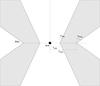 |
Fig. 1 Biconical structure and geometric parameters of the SV disk-wind model. |
With the chosen cylindrical coordinate system, streamline velocities in the wind are given
in the components vr,
vφ and
vz. The velocity along a streamline is
denoted by vl. Then simple geometry gives the relations
vr = vlsinθ
and
vz = vlcosθ.
SV assumed that vl is given by a power law of the length
l = [(r − r0)2 + z2]1/2
along the streamline ![Mathematical equation: \begin{equation} v_{\mathrm{l}} = v_{0} + (v_{\infty} -v_0)\left[\frac{(l/R_{v})^{\alpha}}{(l/R_{v})^{\alpha}+1}\right], \label{eq:SVvl} \end{equation}](/articles/aa/full_html/2014/01/aa21438-13/aa21438-13-eq21.png) (2)where the initial and
asymptotic wind velocities along the streamline v0 and
v∞ are taken as parameters of the model. The two other
parameters in this velocity law are the acceleration scale height of the wind
Rv and α the power-law
constant. In their model SV scaled the asymptotic velocity with local escape velocity at the
streamline base, namely
vesc = (2GMWD/r0)1/2,
with MWD being the mass of the central WD and G
the gravitational constant. As initial velocity they assumed
v0 = 6 km s-1. The wind in the streamlines not
only has a velocity in l direction, but also an orbital velocity
vφ. It is initially given by the Keplerian
motion of the disk at the streamline launching point
vφ,0 = (GMWD/r0)1/2
and is only changed by the assumption of angular momentum conservation around the rotation
axis, leading to
(2)where the initial and
asymptotic wind velocities along the streamline v0 and
v∞ are taken as parameters of the model. The two other
parameters in this velocity law are the acceleration scale height of the wind
Rv and α the power-law
constant. In their model SV scaled the asymptotic velocity with local escape velocity at the
streamline base, namely
vesc = (2GMWD/r0)1/2,
with MWD being the mass of the central WD and G
the gravitational constant. As initial velocity they assumed
v0 = 6 km s-1. The wind in the streamlines not
only has a velocity in l direction, but also an orbital velocity
vφ. It is initially given by the Keplerian
motion of the disk at the streamline launching point
vφ,0 = (GMWD/r0)1/2
and is only changed by the assumption of angular momentum conservation around the rotation
axis, leading to  (3)Shlosman & Vitello (1993) took the mass-loss rate per unit
surface of the disk in the direction of a streamline, ṁ, at the base radius
r0 to be a fraction of the total mass-loss rate by the wind
Ṁwind given by
(3)Shlosman & Vitello (1993) took the mass-loss rate per unit
surface of the disk in the direction of a streamline, ṁ, at the base radius
r0 to be a fraction of the total mass-loss rate by the wind
Ṁwind given by  (4)with the area integral
being over the disk surface between rmin and
rmax, or more explicitly,
(4)with the area integral
being over the disk surface between rmin and
rmax, or more explicitly,
 (5)where the factor of two
accounts for the lower and upper surface of the disk. Although one can accommodate a more
complicated form of mass loss with this formula, SV generally used λ = 0,
which corresponds to a uniform mass loss. As the streamlines connect to the disk at an
angle, the cosθ factor is needed to correct for this.
(5)where the factor of two
accounts for the lower and upper surface of the disk. Although one can accommodate a more
complicated form of mass loss with this formula, SV generally used λ = 0,
which corresponds to a uniform mass loss. As the streamlines connect to the disk at an
angle, the cosθ factor is needed to correct for this.
Shlosman & Vitello (1993) used an unequally
spaced grid in r, z, and θ above and
below the disk. Densities are calculated for each grid cell at the cell center. The density
in the first cell above the disk is given by
 (6)For points farther out in
the wind the values of r0 and
θ(r0) need to be determined first. Simple
geometrical considerations, namely the projection of the θ-run of the
streamlines from a height z to the disk at z = 0, lead to
(6)For points farther out in
the wind the values of r0 and
θ(r0) need to be determined first. Simple
geometrical considerations, namely the projection of the θ-run of the
streamlines from a height z to the disk at z = 0, lead to
 (7)with
 (8)where
rmin,z = rmin + ztanθmin
and
rmax,z = rmax + ztanθmax
are the r values that limit the wind cone at height z.
Then, with given (r, z), r0
and θ(r0), the velocity
v(r,z) = (vr(r,z),vφ(r,z),vz(r,z))
is readily calculated using Eqs. (2) and
(3). The density at (r,
z) can then be calculated from the relation
(8)where
rmin,z = rmin + ztanθmin
and
rmax,z = rmax + ztanθmax
are the r values that limit the wind cone at height z.
Then, with given (r, z), r0
and θ(r0), the velocity
v(r,z) = (vr(r,z),vφ(r,z),vz(r,z))
is readily calculated using Eqs. (2) and
(3). The density at (r,
z) can then be calculated from the relation  (9)As the wind flows
away from the disk, the area between the streamlines increases. This is incorporated in the
above equation via the
(r0/r)(dr0/dr)
term, which is just the area between two streamlines at some height above the disk divided
by the area between these two streamlines on the disk. Taking a geometrical view and keeping
in mind that the distance l along a streamline is
l(r) = z/cosθ(r),
one can derive
(9)As the wind flows
away from the disk, the area between the streamlines increases. This is incorporated in the
above equation via the
(r0/r)(dr0/dr)
term, which is just the area between two streamlines at some height above the disk divided
by the area between these two streamlines on the disk. Taking a geometrical view and keeping
in mind that the distance l along a streamline is
l(r) = z/cosθ(r),
one can derive  (10)Equipped with these
densities and velocities, the wind structure can be calculated easily.
(10)Equipped with these
densities and velocities, the wind structure can be calculated easily.
Additional assumptions of SV are a constant wind temperature of 20 000 K and local ionization equilibrium. They considered H, He, C, N, and O with solar abundances, and solved the radiation transfer in Sobolev approximation. They included a boundary layer as radiation source in their model.
3. Hydrodynamic model for CV winds
Hydrodynamic models of disk winds driven by the radiation force resulting from photon scattering in numerous spectral lines (so-called line driving) have only recently been developed (Feldmeier & Shlosman 1999; Feldmeier et al. 1999; Proga et al. 1998, 1999). The low wind mass-loss rates obtained in these papers revealed that fundamental processes are missing in the treatment. Most likely, these shortcomings stem from in the description of the line-driving force adopted from the CAK theory (Castor et al. 1975) for O star winds, which seems far too simplified for CV winds. The major shortcomings of that theory seem to be the assumptions of no line overlap (induced by Doppler-velocity shifts in the wind) and the highly simplified, two-parameter description of the complex NLTE situation of a relatively thin wind exposed to a strong UV radiation field. At present, we can only adopt results from the hydrodynamic models that agree with reliable empirical results on CV winds, most notably (i) that the wind originates from the inner regions of the accretion disk and is strongly biconical; and (ii) that the calculated wind mass-loss rate is on the order of the single-scattering limit. The role of magnetic torques and forces and of X-ray disk irradiation has to be clarified in future work.
The hydrodynamic models assuming a CAK line force have three unique features. (i) They show a critical point above the disk along a streamline where the flow speed equals that of radiative-acoustic waves (Abbott 1980); (ii) the Euler equation can be put in a form that reflects that of the Laval nozzle flow; (iii) both the mass-loss rate from a narrow disk ring and the inclination of the wind streamline with the disk normal are then uniquely fixed at the location where this nozzle function has its minimum.
The toroidal wind speed is fixed by assuming angular momentum conservation above a Keplerian disk. For the poloidal wind speed, we assumed that the parcel streamline projected onto the poloidal plane can be approximated by a straight line. Whereas the tilt of this wind cone with the disk normal is a fit parameter in the kinematical disk wind models by SV and KWD, it is, according to the above, a fixed (“eigen-”) value in the dynamical model by Feldmeier & Shlosman (1999). Comparing the disk wind structure resulting from hydrodynamic models and the structure assumed in the kinematical models, we see a strong similarity. Using hydrodynamic models, it is therefore possible to fix the free parameters of the kinematical models. Similarly, the radial dependence of the mass-loss rate per disk ring of infinitesimal extent dr (as well as the inner and outer termination radius of the wind) is parameterized in the kinematical models, and is uniquely determined in the dynamical model.
Since the integrated mass-loss rate from the hydrodynamic models is certainly too low, we scaled the latter upwards by an appropriate factor.
With the mass-loss rate leaving the disk in a ring of width dR at location
R,  (11)we follow Feldmeier & Shlosman (1999) to find the Euler
equation
(11)we follow Feldmeier & Shlosman (1999) to find the Euler
equation  (12)with the nozzle function
 (13)Here
Fs is the flux projected onto the
streamline s and C is a constant. The parameter
η was introduced to allow for a general value of α.
(13)Here
Fs is the flux projected onto the
streamline s and C is a constant. The parameter
η was introduced to allow for a general value of α.
The solution “topology” of Eq. (12) can be understood from Fig. 2 (adopted from Fig. 3 in Cassinelli 1979), which shows the line force gl as function of the inertia w′ for three selected values of the mass-loss rate. These curves are concave from below since α < 1. This driving force is in balance with the two retarding forces (plotted positive in the figure), w′ and the projected gravity gs. Note that the inertial force is a 45° diagonal in the diagram, and that gs, depending only on z not w′, is a constant since a fixed yet arbitrary location is considered. The retarding and driving forces cross at either zero, one (open square in the diagram), or two points (closed squares). The latter two correspond to the so-called shallow and steep solutions. If the mass-loss rate adopts the critical CAK value, the shallow and steep solution merge into one. For still higher mass-loss rates, only imaginary solutions are possible, and the wind is called overloaded.
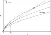 |
Fig. 2 Solution “topology” of the Euler equation, adopted from Cassinelli (1979). w′ and
gs are the two retarding forces,
plotted positive, whose sum crosses the driving force gl
at either zero, one (open square) or two points (closed squares). The line force is
plotted for three values of the mass-loss rate. The critical point
|

At the critical point (subscript c), one therefore has
 (14)or
 (15)This is the famous CAK
critical-point condition. Note that the Euler equation is
w′ + gs − gl = 0,
at every point, hence also at the critical point. This set of two equations
(at the critical point) is readily solved, giving the well-known CAK relations
(15)This is the famous CAK
critical-point condition. Note that the Euler equation is
w′ + gs − gl = 0,
at every point, hence also at the critical point. This set of two equations
(at the critical point) is readily solved, giving the well-known CAK relations
 (16)and
 (17)Requiring
nc = dṀwind, we arrive at
(17)Requiring
nc = dṀwind, we arrive at
 (18)thus the nozzle function is
 (19)This indeed reproduces the
simple α = 1/2 case from before. The unique critical
wind solution is then determined by the (appropriate) saddle point of the function
(19)This indeed reproduces the
simple α = 1/2 case from before. The unique critical
wind solution is then determined by the (appropriate) saddle point of the function
 (20)The effective gravitational
acceleration (gravity minus centrifugal force) above a Keplerian accretion disk along the
s-streamline is given by
(20)The effective gravitational
acceleration (gravity minus centrifugal force) above a Keplerian accretion disk along the
s-streamline is given by
![Mathematical equation: \begin{equation} g_{s}(s) = - GM_{\mathrm{WD}}R \left[ \frac{s/R + \sin\theta}{\left(R^{2}\!+\!2Rs\sin\theta\!+\!s^{2}\right)^{3/2}} - \frac{\sin\theta}{\left(R\!+\!s\sin\theta\right)^{3}} \right]\cdot\! \end{equation}](/articles/aa/full_html/2014/01/aa21438-13/aa21438-13-eq77.png) (21)Closed algebraic
expressions for the radiative flux can only be given in highly simplified cases for the
radial temperature run in the disk, for example, for an isothermal disk and for
T ~ r−1/2, see Feldmeier & Shlosman (1999). The disk with a
T ~ r−1/2 temperature
stratification is called Newtonian in the following. Fortunately, the
radiation field from a narrow ring emitting as a black body can be calculated analytically,
and thus the disk emission be obtained from a 1D numerical integration. The nozzle function
obtained from this, along with the relevant saddle points, is shown in Fig. 6 of Feldmeier & Shlosman (1999), and the relevant
eigenvalues for θ are given in their Table 1. Note that
λcr = 90°−θc is
tabulated there. The value of the nozzle function itself at the saddle, that is, the
critical mass-loss rate, is given in the same table, and is shown as function of footpoint
radius in Fig. 3. Note that in Shlosman & Vitello (1993), the mass-loss rate from a disk ring is
taken as proportional to the ring area RdR. This is a
severe approximation, and the current eigenvalue or nozzle analysis allows us to
derive the mass-loss rate from a ring as a function of its radius.
(21)Closed algebraic
expressions for the radiative flux can only be given in highly simplified cases for the
radial temperature run in the disk, for example, for an isothermal disk and for
T ~ r−1/2, see Feldmeier & Shlosman (1999). The disk with a
T ~ r−1/2 temperature
stratification is called Newtonian in the following. Fortunately, the
radiation field from a narrow ring emitting as a black body can be calculated analytically,
and thus the disk emission be obtained from a 1D numerical integration. The nozzle function
obtained from this, along with the relevant saddle points, is shown in Fig. 6 of Feldmeier & Shlosman (1999), and the relevant
eigenvalues for θ are given in their Table 1. Note that
λcr = 90°−θc is
tabulated there. The value of the nozzle function itself at the saddle, that is, the
critical mass-loss rate, is given in the same table, and is shown as function of footpoint
radius in Fig. 3. Note that in Shlosman & Vitello (1993), the mass-loss rate from a disk ring is
taken as proportional to the ring area RdR. This is a
severe approximation, and the current eigenvalue or nozzle analysis allows us to
derive the mass-loss rate from a ring as a function of its radius.
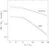 |
Fig. 3 Mass-loss rate per disk annulus,
dṀwind/dr0,
as a function of the footpoint radius. Data for
α = 2/3 and
α = 1/2 were used for both Newtonian and
α-disks. Fits with |


The wind starts roughly at three WD radii (RWD) from the disk center. Farther in, details of wind launching are currently unknown because of the complexity of the disk boundary layer, the disk corona, etc. Interestingly, in the wind models of Feldmeier & Shlosman (1999), who adopted a Shakura & Sunyaev (1973)α-disk, no appropriate saddle point of the nozzle function and hence no critical wind solution is found inside ≈3 RWD.
For the outer wind termination radius in the disk, we do not follow the conclusion in Feldmeier et al. (1999) that the total mass-loss rate is
dominated by the inner wind up to 7 RWD, for instance, and
that regions farther out can be neglected. Instead, Fig. 3 indicates that the region in the disk from ten to thirty
RWD should contribute roughly one third of the total mass-loss
rate. For r > 5 RWD,
Feldmeier et al. (1999) found a power-law dependence
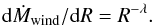 (22)An approximate value
for λ can be estimated from Eq. (19) by considering the R-dependence of the nozzle function in the
near disk regime (s → 0). Obviously then, gravity
g ~ R-2, and flux F resp.
intensity
IF ~ I4 ~ R-2
to R-3, where in the latter relation the outer regions of either
a Newtonian or α-disk are assumed. From Eq. (19),
dṀwind/dR ~ R-1
follows (in Feldmeier et al. 1999:
R-0.8) for the Newtonian disk and either
α = 1/2 or 2/3; and
dṀwind/dR ~ R-3
resp. R-2.5 for the α-disk and
α = 1/2 resp. 2/3 (in Feldmeier et al. 1999: R-1.9
for both α). In our wind models, we adopted the values for
λ from Feldmeier et al. (1999).
(22)An approximate value
for λ can be estimated from Eq. (19) by considering the R-dependence of the nozzle function in the
near disk regime (s → 0). Obviously then, gravity
g ~ R-2, and flux F resp.
intensity
IF ~ I4 ~ R-2
to R-3, where in the latter relation the outer regions of either
a Newtonian or α-disk are assumed. From Eq. (19),
dṀwind/dR ~ R-1
follows (in Feldmeier et al. 1999:
R-0.8) for the Newtonian disk and either
α = 1/2 or 2/3; and
dṀwind/dR ~ R-3
resp. R-2.5 for the α-disk and
α = 1/2 resp. 2/3 (in Feldmeier et al. 1999: R-1.9
for both α). In our wind models, we adopted the values for
λ from Feldmeier et al. (1999).
The critical angle θc varies only marginally in the wind-launching area. We adopted the values for the different disk models calculated by Feldmeier & Shlosman (1999) as shown in their Table 1. For r0 ≈ 3 RWD they found θc = 25°...27° and for the outer edge of the wind at r0 ≈ 30 RWD they found θc = 33°...39°. The influence on the resulting spectra of such a minor variation in θc is negligible compared with the other uncertainties in the model. We therefore adopted a simple linear variation of θc from 25° to 35° as r0 varies from 3 RWD to 30 RWD.
4. Monte Carlo radiative transfer
We have developed a Monte Carlo based code to calculate radiative transfer in three
dimensions (WoMPaT). The two wind models described above are implemented. We use
photon packets with energy weights in our implementation, where
wi represents the weight of the
i-th photon. A weight of w = 1 corresponds to an energy
 (23)where
Npp corresponds to the total number of photons and
Etot to the total energy of all photons used in the
simulation. We also use the weights as a method of keeping the Monte Carlo noise equal for
each frequency bin, therefore the weights have to be adjusted as
(23)where
Npp corresponds to the total number of photons and
Etot to the total energy of all photons used in the
simulation. We also use the weights as a method of keeping the Monte Carlo noise equal for
each frequency bin, therefore the weights have to be adjusted as
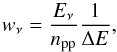 (24)where
Eν is the total energy in the frequency bin
ν and npp the number of photons in that bin,
the factor 1/ΔE normalizes the weight with respect to
the w = 1 case. Because we then use exactly the same number of photons for
each frequency bin, the initial frequency bin is not randomly sampled, only the initial
photon frequency in this bin is sampled from a linear distribution.
(24)where
Eν is the total energy in the frequency bin
ν and npp the number of photons in that bin,
the factor 1/ΔE normalizes the weight with respect to
the w = 1 case. Because we then use exactly the same number of photons for
each frequency bin, the initial frequency bin is not randomly sampled, only the initial
photon frequency in this bin is sampled from a linear distribution.
Photons are either created on the WD with a probability
pWD = EWD/Etot
or at the disk surface with a probability
pdisk = Edisk/Etot.
A boundary layer as radiation source is not included. If a photon is created on the WD, the
initial position on the WD surface is completely random. The initial direction is determined
with respect to the local outward normal and then transformed back to the standard
coordinate system with the origin at the WD center. In local polar coordinates, the initial
direction is given by  .
The probability to emit in a solid angle
dω = sinθdθdφ is given
by
.
The probability to emit in a solid angle
dω = sinθdθdφ is given
by  (25)where
η(θ) is the standard limb darkening in Eddington
approximation and cosθ is a geometric factor accounting for the
foreshortening of the emitting surface. The sinθ factor is purely due to
the spherical coordinates and later again comes into play when the flux per solid angle
Iν/dω is
calculated from the photon bins. Obviously, the φ-direction is arbitrary
and as such is sampled by φ = ζ2π, where
ζ is a pseudo-random number drawn from a uniform distribution between
zero and one.
(25)where
η(θ) is the standard limb darkening in Eddington
approximation and cosθ is a geometric factor accounting for the
foreshortening of the emitting surface. The sinθ factor is purely due to
the spherical coordinates and later again comes into play when the flux per solid angle
Iν/dω is
calculated from the photon bins. Obviously, the φ-direction is arbitrary
and as such is sampled by φ = ζ2π, where
ζ is a pseudo-random number drawn from a uniform distribution between
zero and one.
If a photon is created on the disk surface, the initial position is given by
rinit = (ri,φi,zi)
in cylindrical coordinates. It is zi = 0 because the disk is
taken to be infinitesimally thin, furthermore, the disk is axisymmetric, thus
φi = ζ2π. The initial radial
position ri is found via a lookup table from the cumulative
distribution function 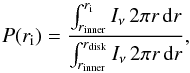 (26)where
rdisk is the radius of the accretion disk and
Iν = Iν(θ = 0)
the intensity in the frequency bin at ν. The initial direction
(26)where
rdisk is the radius of the accretion disk and
Iν = Iν(θ = 0)
the intensity in the frequency bin at ν. The initial direction
 is found in the same way as for emission on the WD.
The next step is to determine whether and where a photon interacts. For this the optical depth along the line of flight (LOF) is calculated by integrating the opacities via a trapezium rule with transformations into the co-moving frame at each integration point. Velocity gradients are taken into consideration. Opacities include bound-bound, bound-free, free-free, and electron scattering, although it was found that only the line opacities are important. All opacities are computed in LTE approximation. Generalization to NLTE is devoted to future work.
After this integration we not only know the total optical depth
τtot for this LOF in the medium, but also the run of the
optical depth τ = τ(s) as a function of
the distance s along the LOF. From the definition of the optical depth, the
probability that the photon escapes from the medium is given by
 (27)then the
probability that the photon scatters is given by
(27)then the
probability that the photon scatters is given by
 (28)If the sampled random
number ζ < pesc, then
the photon escapes the medium, otherwise it scatters at an optical depth of
(28)If the sampled random
number ζ < pesc, then
the photon escapes the medium, otherwise it scatters at an optical depth of ![Mathematical equation: \begin{equation} \label{eq:tauscat} \tau_{\mathrm{scat}} = - \ln [ 1 - \zeta ( 1 - {\rm e}^{-\tau_{\mathrm{tot}}})] . \end{equation}](/articles/aa/full_html/2014/01/aa21438-13/aa21438-13-eq149.png) (29)After calculating
τscat, the point s along the LOF (and thus
the location rscat) where this optical depth is
reached and the scattering process occurs is easily determined by inverting
τ(s).
(29)After calculating
τscat, the point s along the LOF (and thus
the location rscat) where this optical depth is
reached and the scattering process occurs is easily determined by inverting
τ(s).
The escape of the photon can be implemented in two ways. The straightforward way is to really determine whether the photon leaves the wind or not, and if it leaves the wind, then it really leaves the simulation volume and “dies”, if it remains in the wind, the whole photon weight remains in the wind. This is called a “live or die” algorithm. On the other hand, the notion of weights allows at this point for an algorithm referred to as “forced scattering”. A part of the photon is taken to always scatter in the medium and a part of the photon, namely the one with the weight wesc = wpesc, escapes and is detected. In this case ζ does not determine if scattering occurs, but only determines the point where scattering for the photon with the reduced weight wnew = wpscat occurs via Eq. (29). This technique is based on the assumption that a photon is really a photon packet consisting of many photons out of which a certain part would actually exhibit this behavior and escape and another part would remain in the medium. Such an algorithm is used to reduce the noise of the simulation and has been used in a Monte Carlo simulation of accretion disk winds by Knigge et al. (1995).
After the scattering location is known, and also whether and in which line the scattering
occurs, which is of course not determined probabilistically, all there remains to be done is
to assign the photon a new frequency νnew and a new direction
 ,
both are taken to be independent of the incident νold and
,
both are taken to be independent of the incident νold and
 .
For line scattering the new direction is drawn from a spherically isotropic distribution and
the new frequency is drawn from a Gaussian in the co-moving frame and then transformed into
the rest frame. Therefore the new frequency is given by
.
For line scattering the new direction is drawn from a spherically isotropic distribution and
the new frequency is drawn from a Gaussian in the co-moving frame and then transformed into
the rest frame. Therefore the new frequency is given by
![Mathematical equation: \begin{equation} \nu_{\mathrm{new}} = (\nu_{0} + \xi \Delta \nu_{\mathrm{D}})\left[ 1 + \frac{\boldsymbol{v}(\boldsymbol{r}_{\mathrm{scat}}) \cdot \boldsymbol{\hat{d}}_{\mathrm{new}}} {c}\right] , \end{equation}](/articles/aa/full_html/2014/01/aa21438-13/aa21438-13-eq159.png) (30)where ξ is
a random number sampled from a Gaussian distribution with mean zero and standard deviation
unity, c is the speed of light, and ν0 and
ΔνD are the rest frequency and the Doppler width of the line
in which scattering occurs, respectively. Our main concerns are strong resonance lines,
therefore we take the line scattering as 100% efficient. Bound-free and free-free processes
are ignored, that is, only electron scattering is taken into account. It is assumed to be
coherent and isotropic.
(30)where ξ is
a random number sampled from a Gaussian distribution with mean zero and standard deviation
unity, c is the speed of light, and ν0 and
ΔνD are the rest frequency and the Doppler width of the line
in which scattering occurs, respectively. Our main concerns are strong resonance lines,
therefore we take the line scattering as 100% efficient. Bound-free and free-free processes
are ignored, that is, only electron scattering is taken into account. It is assumed to be
coherent and isotropic.
Using a Sobolev approach would be computationally less expensive, but there are some limitations. Multiple scattering in the resonance region is neglected, there is only one interaction per resonance surface. In wind situations with a non-monotonic velocity law Sobolev calculations are still feasible, but become more complicated. As the resonance surfaces are taken to be sharp, physical quantities are assumed to be constant on the resonance surface. The assumption of a finite resonance region in which physical quantities are allowed to change is more realistic. In cases where more effects such as line overlap or wind clumping have to be considered, it is better to drop the Sobolev approximation and adopt accurate methods such as co-moving frame calculations (see e.g. Hillier et al. 2003). This method is based on a transformation into the co-moving frame at which the local medium is at rest. Opacities and emissivities are isotropic in this frame, the anisotropy is taken care of by the frame transformation. Numerical integration of the radiative transfer equation, or integration of the opacities, requires a frame transformation at every sampling point with this method (see e.g. Knigge et al. 1995). Such a method is more expensive, but can reveal differences with respect to the Sobolev method, for example, a comparison of co-moving frame methods and Sobolev methods for O and WR star winds yield differences in wind acceleration and clumping factors (Hillier et al. 2003; Gräfener & Hamann 2005; and Gräfener 2007, priv. comm.). In a Monte Carlo context opacity calculations using a co-moving frame method are a tractable problem (Knigge et al. 1995), where the trade-off in run time with current computer power to the gained insight from a comparison with older Sobolev results is obvious. We therefore implemented a co-moving frame method in this work.
5. Accretion disk code AcDc
To calculate the metal-line blanketed NLTE accretion-disk models, which are input models
for the wind calculations, we used our accretion-disk code AcDc (Nagel et al. 2004). It is based on the radial structure
of an α-disk (Shakura & Sunyaev
1973), assuming a stationary, geometrically thin disk (the total disk thickness
H is much smaller than the disk diameter). This allows the decoupling of
the vertical and radial structures and, assuming axial symmetry, we can separate the disk
into concentric annuli of plane-parallel geometry. In that way, the radiative transfer
becomes a 1d problem. The radial distribution of the effective temperature
Teff can be described by ![Mathematical equation: \begin{equation} T_{\mathrm{eff}}(R) = \left[\frac{3GM_{\mathrm{WD}}\dot{M}_{\mathrm{disk}}}{8\pi\sigma R^{3}}\left(1 - \sqrt{\frac{R_{\mathrm{WD}}}{R}}\right) \right]^{1/4}\,, \label{tglg} \end{equation}](/articles/aa/full_html/2014/01/aa21438-13/aa21438-13-eq166.png) (31)where
Ṁdisk denotes the mass-accretion rate through the disk and
σ is the Stefan-Boltzmann constant.
(31)where
Ṁdisk denotes the mass-accretion rate through the disk and
σ is the Stefan-Boltzmann constant.
For each disk ring, the following set of coupled equations were solved simultaneously under the constraints of particle number and charge conservation:
-
radiation transfer for the specific intensity I,
-
hydrostatic equilibrium between gravitation, gas pressure Pgas, and radiation pressure,
-
energy balance between the viscously generated energy Emech and the radiative energy loss Erad,
-
NLTE rate equations for the population numbers ni of the atomic levels i.
6. Spectral properties of kinematical and hydrodynamic models
We tested the influence of the wind temperatures as well as the influence of the size of the computational domain on the calculated spectrum in the case of a standard SV (Table 1) and a standard hydrodynamic model (Table 2).
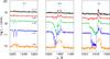 |
Fig. 4 Standard SV model spectra for Twind = 20 000 K on a large domain. Note the prominent C iv 1550 Å and Si iv 1400 Å lines while N v 1240 Å is absent. |
Standard parameter set for the SV model.
Standard parameter set for the hydrodynamic wind model.
6.1. Standard SV model
The calculated spectra for a constant wind temperature of 20 000 K show a very prominent C iv line at 1550 Å. Depending on the inclination angle, it shows an absorption, emission, or P Cygni profile. Another strong feature is the Si iv line at 1400 Å, showing the same profiles as the carbon line. The N v line at 1240 Å is missing because of the low wind temperature (Fig. 4, all calculated spectra here and in the following figures of this section are folded with a 0.3 Å Gaussian.).
For a constant wind temperature of 40 000 K the strength of the C iv and Si iv lines decrease, but the N v line at 1240 Å is strong and shows a P Cygni profile for intermediate inclination angles (Fig. 5).
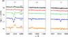 |
Fig. 5 Same as Fig. 4, but for Twind = 40 000 K. Note the prominent N v 1240 Å line, while C iv 1550 Å and Si iv 1400 Å are very weak. |
Different sizes of the computational domain affect the spectra (Fig. 6, lower panel). The width of the absorption troughs is broader for the larger domain (cylinder with radius and height of 2000 RWD) than for the small domain (cylinder with radius and height of 100 RWD). We conclude that there is absorbing material in the lines even beyond the small domain. These faster-moving parts of the wind are missed using the small domain, and hence, the lines are narrower. Therefore, it is necessary to use the larger domain. For an even larger domain of 20 000 RWD, the width of the absorption troughs does not change any further than for the 2000 RWD case. A grid with 100 × 100 boxes resolves the lines slightly better than a 30 × 30 grid (Fig. 6, upper panel), but the significantly higher demands in memory and computation time are not justified by the small difference.
Especially for the cooler model, the spectra show narrow emission and absorption spikes. They are limited to only one frequency point at the rest wavelength of a spectral line. We interpret them as numerical artifacts, but their origin remains unclear.
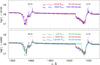 |
Fig. 6 Comparison of the C iv 1550 Å and Si iv 1400 Å lines for SV models with 20 000 K wind temperature, different computational domain sizes (lower panel), and different numbers of boxes (upper panel) for i = 45°. Note, that the lines for the larger domain are broader. |
6.2. Standard hydrodynamic model
The calculations for the standard hydrodynamic model show similar results as for the standard SV model. The main difference for a constant wind temperature of 20 000 K is that the C iv 1550 Å and Si iv 1400 Å lines have a narrower absorption trough and show a double-peaked profile for high inclination angles (Fig. 7). For a constant wind temperature of 40 000 K the N v 1240 Å line is narrower than in the SV model (Fig. 8). These differences are probably due to the higher collimation of the wind for the hydrodynamic model. Artificial spikes as in the SV model are much less pronounced.
7. AM CVn: wind modeling
AM CVn, the prototype system for the class of AM CVn stars, is a hydrogen-deficient nova-like CV (Downes et al. 1997). The orbital period is 1029 s (Harvey et al. 1998). For primary and secondary masses there are several values in discussion, with the most agreed upon being MWD ≈ 0.7 M⊙ and M2 ≈ 0.1 M⊙ (Roelofs et al. 2007). However, using synthetic spectra of a large grid of accretion-disk models (Nagel et al. 2009) calculated with AcDc, we found the best agreement with observation for models with MWD = 0.6 M⊙ and an accretion rate Ṁ = 1 × 10⁻⁸ M⊙ yr-1. Therefore these parameters were adopted for the study of AM CVn wind spectra in this work. The corresponding WD radius is RWD = 9550 km. As accretion-disk extension we considered rin = 1.36 RWD to rout = 14.66 RWD, where the outer radius rout of the disk corresponds roughly to the tidal radius. The best agreement with observations for the disk models is found for an inclination of about 40° (Nagel et al. 2004; Roelofs et al. 2007).
We used an SV model for the wind calculations with the parameter set as given in Table 3. The chemical composition is helium-dominated with solar abundances of C, O, and Si, two different values for N, and no hydrogen. The calculations were performed on the high-performance cluster of the University of Tübingen, using up to 64 cores and 200 million photon packages. We compared our calculated model spectra with an observed spectrum taken by HST/STIS (Wade et al. 2007).
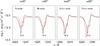 |
Fig. 9 Comparison of the calculated N v resonance line (SV model) with an observed spectrum of AM CVn. The STIS observation is plotted in black in each panel, the calculated lines (Twind = 40 000 K, Ṁwind = 1 × 10⁻⁹ M⊙ yr-1) are drawn in red. |
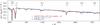 |
Fig. 10 HST/STIS spectrum of AM CVn (black), disk spectrum (blue), and wind spectrum (red, Twind = 35 000 K, Ṁwind = 5 × 10⁻¹⁰ M⊙ yr-1, SV model). Note the prominent P Cygni profile of the N v 1240 Å line is not similar to that of the disk, but to that of the wind model. All models are reddened by E(B − V) = 0.12, and folded with a 1.2 Å Gaussian. |
Parameter set of the SV wind model for AM CVn.
A first model with a constant wind temperature of 40 000 K and either solar (left two panels) or five times solar N abundance (right two panels) is shown in Fig. 9. The wind model spectra indicate the observed P Cygni profile of the N v doublet around 1240 Å, but neither the model for an inclination of i = 40°, nor the model for i = 60° gives a satisfying fit for a mass-loss rate of 1 × 10⁻⁹ M⊙ yr-1. In both cases the computed profile is not broad and deep enough. We chose these two inclinations because the first is the most probable value discussed in the literature and the latter is the most extreme inclination that might still be possible. As for some AM CVn systems a high abundance of nitrogen is reported, for example, GP Com (Morales-Rueda et al. 2003) or V396 Hya (Ramsay et al. 2006), we calculated a wind spectrum with the nitrogen abundance increased to five times solar. The resulting N v line is generally deeper, the model matches the observed spectrum better for i = 40°. However, one has to keep in mind that there are other parameters that might influence the resulting spectrum, for instance, those describing the wind geometry, which have not been investigated, as well as other nitrogen abundances.
A closer comparison of the N v 1240 Å doublet and the C iv 1550 Å doublet with the observed STIS spectrum was performed for the 30 × 30 grid on the large computational domain for four different wind temperatures (30 000 K, 35 000 K, 40 000 K, and 45 000 K) and for three mass-loss rates (5 × 10⁻¹⁰, 1 × 10⁻⁹, and 5 × 10⁻⁹ M⊙ yr-1). The nitrogen abundance was set to five times solar. Results for i = 40° are plotted in Figs. 12 and 13, those for i = 60° in Figs. 14 and 15. For i = 40°, the N v line is best reproduced by combining a wind temperature of 40 000 K and a mass-loss rate of 1 × 10⁻⁹ M⊙ yr-1 or a wind temperature of 35 000 K and a mass-loss rate of 5 × 10⁻¹⁰ M⊙ yr-1. For higher and lower wind temperatures, the line is too weak. Furthermore, a higher mass-loss rate results in a too broad absorption trough. For i = 60°, the same is true: the best agreement with the observation is found for a wind temperature of 40 000 K and a mass-loss rate of 5 × 10⁻¹⁰ M⊙ yr-1. Generally, the spectral line is broader and deeper than for i = 40°.
For the C iv line, the lowest wind temperature can be excluded for all mass-loss rates and both inclinations because the resulting line profile is too deep. Moreover, none of the models for i = 60° and wind temperature of 35 000 K or highest mass-loss rate results in satisfying line profiles. For i = 40°, a good agreement with observation is obtained for a wind temperature of 35 000 K and a mass-loss rate between 5 × 10⁻¹⁰ and 1 × 10⁻⁹ M⊙ yr-1.
The discrepancies in the parameter values needed to match the C iv and N v lines indicate a non-isothermal wind structure, as shown for example by Long & Knigge (2002) or Noebauer et al. (2010) for several CVs. A different mass-loss rate for different species is unlikely, the correct value is probably between 1 × 10⁻⁹ M⊙ yr-1 and 5 × 10⁻¹⁰ M⊙ yr-1.
In Fig. 10 we show the observed UV spectrum, our best-fit SV model for the wind (Ṁwind = 5 × 10⁻¹⁰ M⊙ yr-1, Twind = 35 000 K, i = 40°), and an accretion-disk model. The wind model reproduces the observed spectrum much better than the pure disk spectrum. Both synthetic spectra are reddened by E(B − V) = 0.12. Calculating a hydrodynamic model for the same parameters, the result looks similar. The C iv 1550 Å line is deeper, matching the depth of the observed line better. Unfortunately, the model spectrum does not show the emission peak of the N v 1240 Å line, which is well reproduced in the SV model.
Not all lines in the observed spectrum are produced by the accretion-disk wind. Figure 11 shows that with a multi color blackbody disk as input for the wind calculation especially the Si iv line cannot be reproduced as well as with an NLTE accretion-disk spectrum as input, whereas the N v line is a pure wind line.
8. Conclusions
We have performed 2.5D Monte Carlo radiative transfer calculations with LTE opacities in hydrodynamic wind structures using NLTE spectra from the accretion disk as input and accounting for the white dwarf as an additional photon source. Our main conclusions are listed below.
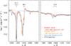 |
Fig. 11 HST/STIS spectrum of AM CVn (black) compared with a wind spectrum with an NLTE accretion-disk model spectrum as input (red) and a wind spectrum with a multi-color blackbody spectrum as input (orange). In blue, the pure NLTE disk spectrum is shown. |
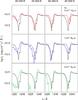 |
Fig. 12 Comparison of the calculated N v 1240 Å line (i = 40°, SV model) with the STIS observation (black). |
-
Sampling the accretion-disk wind by a 30 × 30 grid is sufficient for a good resolution of the wind lines. But it is necessary to extend the computational domain up to 2000 RWD instead of only a few hundred to include faster-moving absorbing material farther out that contributes significantly to the line widths.
-
The two accretion-disk wind descriptions implemented in WoMPaT produce similar line profiles. The major difference between kinematical and hydrodynamic wind models are narrower lines in the hydrodynamic models due to the used wind geometry.
-
Applying our WoMPaT code to model the helium “nova-like” AM CVn has been successful in reproducing the prominent P Cygni profiles, which our disk models lacked up to now. Comparing our SV model calculations to UV observations of AM CVn, we found the best agreement for Ṁwind = 5 × 10⁻¹⁰ M⊙ yr-1 and Twind = 35 000 K using the most probable literature value of i = 40° for the system inclination. However, the N abundance had to be five times solar to model the line strength of the N v line at about 1240 Å.
Furthermore, our results show the necessity of a variable temperature structure in the wind, such as Long & Knigge (2002) or Noebauer et al. (2010) use in their models, to reproduce different wind lines with the same quality. This will be one of the first steps in the future development of our wind code.
bwGRiD (http://www.bw-grid.de), member of the German D-Grid initiative, funded by the Ministry for Education and Research (Bundesministerium für Bildung und Forschung) and the Ministry for Science, Research and Arts Baden-Württemberg (Ministerium für Wissenschaft, Forschung und Kunst Baden-Württemberg).
Acknowledgments
This work was supported by DFG grants Fe 477/3-1 and We 1312/37-1. We thank the bwGRiD project1 for the computational resources. We thank the referee for his/her constructive criticism that helped to improve the paper.
References
- Abbott, D. C. 1980, ApJ, 242, 1183 [NASA ADS] [CrossRef] [Google Scholar]
- Cassinelli, J. P. 1979, ARA&A, 17, 275 [NASA ADS] [CrossRef] [Google Scholar]
- Castor, J. I., Abbott, D. C., & Klein, R. I. 1975, ApJ, 195, 157 [NASA ADS] [CrossRef] [Google Scholar]
- Cordova, F. A., & Mason, K. O. 1982, ApJ, 260, 716 [NASA ADS] [CrossRef] [Google Scholar]
- Downes, R., Webbink, R. F., & Shara, M. M. 1997, PASP, 109, 345 [NASA ADS] [CrossRef] [Google Scholar]
- Feldmeier, A., & Shlosman, I. 1999, ApJ, 526, 344 [NASA ADS] [CrossRef] [Google Scholar]
- Feldmeier, A., Shlosman, I., & Vitello, P. 1999, ApJ, 526, 357 [NASA ADS] [CrossRef] [Google Scholar]
- Gräfener, G., & Hamann, W.-R. 2005, A&A, 432, 633 [NASA ADS] [CrossRef] [EDP Sciences] [Google Scholar]
- Harvey, D. A., Skillman, D. R., Kemp, J., et al. 1998, ApJ, 493, L105 [NASA ADS] [CrossRef] [Google Scholar]
- Heap, S. R., Boggess, A., Holm, A., et al. 1978, Nature, 275, 385 [NASA ADS] [CrossRef] [Google Scholar]
- Hillier, D. J., Lanz, T., Heap, S. R., et al. 2003, ApJ, 588, 1039 [NASA ADS] [CrossRef] [Google Scholar]
- Knigge, C., Woods, J. A., & Drew, J. E. 1995, MNRAS, 273, 225 [NASA ADS] [Google Scholar]
- Kusterer, D.-J. 2008, Ph.D. Thesis, University of Tübingen, Germany [Google Scholar]
- Long, K. S., & Knigge, C. 2002, ApJ, 579, 725 [NASA ADS] [CrossRef] [Google Scholar]
- Morales-Rueda, L., Marsh, T. R., Steeghs, D., et al. 2003, A&A, 405, 249 [NASA ADS] [CrossRef] [EDP Sciences] [Google Scholar]
- Nagel, T., Dreizler, S., Rauch, T., & Werner, K. 2004, A&A, 428, 109 [NASA ADS] [CrossRef] [EDP Sciences] [Google Scholar]
- Nagel, T., Rauch, T., & Werner, K. 2009, A&A, 499, 773 [NASA ADS] [CrossRef] [EDP Sciences] [Google Scholar]
- Noebauer, U. M., Long, K. S., Sim, S. A., & Knigge, C. 2010, ApJ, 719, 1932 [NASA ADS] [CrossRef] [Google Scholar]
- Proga, D., Stone, J. M., & Drew, J. E. 1998, MNRAS, 295, 595 [NASA ADS] [CrossRef] [Google Scholar]
- Proga, D., Stone, J. M., & Drew, J. E. 1999, MNRAS, 310, 476 [NASA ADS] [CrossRef] [Google Scholar]
- Puebla, R. E., Diaz, M. P., Hillier, D. J., & Hubeny, I. 2011, ApJ, 736, 17 [NASA ADS] [CrossRef] [Google Scholar]
- Ramsay, G., Groot, P. J., Marsh, T., et al. 2006, A&A, 457, 623 [NASA ADS] [CrossRef] [EDP Sciences] [Google Scholar]
- Roelofs, G. H. A., Groot, P. J., Benedict, G. F., et al. 2007, ApJ, 666, 1174 [NASA ADS] [CrossRef] [Google Scholar]
- Shakura, N. I., & Sunyaev, R. A. 1973, A&A, 24, 337 [NASA ADS] [Google Scholar]
- Shlosman, I., & Vitello, P. 1993, ApJ, 409, 372 [NASA ADS] [CrossRef] [Google Scholar]
- Solheim, J.-E. 2010, PASP, 122, 1133 [NASA ADS] [CrossRef] [Google Scholar]
- Wade, R. A., Eracleous, M., & Flohic, H. M. L. G. 2007, AJ, 134, 1740 [NASA ADS] [CrossRef] [Google Scholar]
All Tables
All Figures
|
Fig. 1 Biconical structure and geometric parameters of the SV disk-wind model. |
| In the text | |
|
Fig. 2 Solution “topology” of the Euler equation, adopted from Cassinelli (1979). w′ and
gs are the two retarding forces,
plotted positive, whose sum crosses the driving force gl
at either zero, one (open square) or two points (closed squares). The line force is
plotted for three values of the mass-loss rate. The critical point
|
| In the text | |
|
Fig. 3 Mass-loss rate per disk annulus,
dṀwind/dr0,
as a function of the footpoint radius. Data for
α = 2/3 and
α = 1/2 were used for both Newtonian and
α-disks. Fits with |
| In the text | |
|
Fig. 4 Standard SV model spectra for Twind = 20 000 K on a large domain. Note the prominent C iv 1550 Å and Si iv 1400 Å lines while N v 1240 Å is absent. |
| In the text | |
|
Fig. 5 Same as Fig. 4, but for Twind = 40 000 K. Note the prominent N v 1240 Å line, while C iv 1550 Å and Si iv 1400 Å are very weak. |
| In the text | |
|
Fig. 6 Comparison of the C iv 1550 Å and Si iv 1400 Å lines for SV models with 20 000 K wind temperature, different computational domain sizes (lower panel), and different numbers of boxes (upper panel) for i = 45°. Note, that the lines for the larger domain are broader. |
| In the text | |
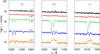 |
Fig. 7 Same as Fig. 4, but for the standard hydrodynamic model. |
| In the text | |
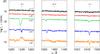 |
Fig. 8 Same as Fig. 5, but for the standard hydrodynamic model. |
| In the text | |
|
Fig. 9 Comparison of the calculated N v resonance line (SV model) with an observed spectrum of AM CVn. The STIS observation is plotted in black in each panel, the calculated lines (Twind = 40 000 K, Ṁwind = 1 × 10⁻⁹ M⊙ yr-1) are drawn in red. |
| In the text | |
|
Fig. 10 HST/STIS spectrum of AM CVn (black), disk spectrum (blue), and wind spectrum (red, Twind = 35 000 K, Ṁwind = 5 × 10⁻¹⁰ M⊙ yr-1, SV model). Note the prominent P Cygni profile of the N v 1240 Å line is not similar to that of the disk, but to that of the wind model. All models are reddened by E(B − V) = 0.12, and folded with a 1.2 Å Gaussian. |
| In the text | |
|
Fig. 11 HST/STIS spectrum of AM CVn (black) compared with a wind spectrum with an NLTE accretion-disk model spectrum as input (red) and a wind spectrum with a multi-color blackbody spectrum as input (orange). In blue, the pure NLTE disk spectrum is shown. |
| In the text | |
|
Fig. 12 Comparison of the calculated N v 1240 Å line (i = 40°, SV model) with the STIS observation (black). |
| In the text | |
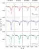 |
Fig. 13 Same as Fig. 12, but for C iv 1550 Å. |
| In the text | |
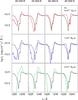 |
Fig. 14 Same as Fig. 12, but for i = 60°. |
| In the text | |
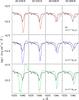 |
Fig. 15 Same as Fig. 13, but for i = 60°. |
| In the text | |
Current usage metrics show cumulative count of Article Views (full-text article views including HTML views, PDF and ePub downloads, according to the available data) and Abstracts Views on Vision4Press platform.
Data correspond to usage on the plateform after 2015. The current usage metrics is available 48-96 hours after online publication and is updated daily on week days.
Initial download of the metrics may take a while.