| Issue |
A&A
Volume 665, September 2022
|
|
|---|---|---|
| Article Number | A139 | |
| Number of page(s) | 16 | |
| Section | Cosmology (including clusters of galaxies) | |
| DOI | https://doi.org/10.1051/0004-6361/202244358 | |
| Published online | 20 September 2022 | |
Accretion flows around exotic tidal wormholes
I. Ray-tracing
1
Astronomical Observatory of the National Academy of Sciences of Ukraine (MAO NASU), Kyiv 03143, Ukraine
2
Astronomical Observatory, Taras Shevchenko National University of Kyiv, 3 Observatorna St., 04053 Kyiv, Ukraine
3
Department of Mathematics, Birla Institute of Technology and Science-Pilani, Hyderabad Campus, Hyderabad 500078, India
e-mail: This email address is being protected from spambots. You need JavaScript enabled to view it.
Received:
27
June
2022
Accepted:
18
July
2022
Abstract
Aims. This paper investigates the various spherically symmetric wormhole solutions in the presence of tidal forces and applies numerous methods, such as test particle orbital dynamics, ray-tracing, and microlensing.
Methods. We make theoretical predictions on the test particle orbital motion around the tidal wormholes with the use of the effective potential normalized by ℒ2. In order to obtain the ray-tracing images of both geometrically thin and thick accretion disks and relativistic jets, we modified the open source GYOTO code using a python interface.
Results. We applied this technique to probe the accretion flows near Schwarzschild-like and charged Reissner-Nordström (RN) wormholes; we assumed both a charged RN wormhole and a special case with a vanishing electromagnetic charge, namely the Damour-Solodukhin (DS) wormhole. We show that the photon sphere for the Schwarzschild-like wormhole present for both thin and thick accretion disks, even for the vanishing tidal forces. Moreover, we observe that rph → ∞ as α → ∞, which constraints the α parameter to be sufficiently small and positive in order to respect Event Horizon Telescope observations. On the other hand, for the case of the RN wormhole, the photon sphere radius shrinks as Λ → ∞, as predicted by the effective potential. In addition to the accretion disks, we also probe the relativistic jets around the two wormhole solutions under consideration. Finally, with the help of star bulb microlensing, we approximate the radius of the wormhole shadow and find that for the Schwarzschild wormhole, RSh ≈ r0 for zero tidal forces and grows linearly with α. On the contrary, the shadow radius for charged wormholes slowly decreases with the growing DS parameter, Λ.
Key words: accretion, accretion disks / gravitational lensing: weak / Galaxy: disk / cosmology: theory
© O. Sokoliuk et al. 2022
 Open Access article, published by EDP Sciences, under the terms of the Creative Commons Attribution License (https://creativecommons.org/licenses/by/4.0), which permits unrestricted use, distribution, and reproduction in any medium, provided the original work is properly cited.
This article is published in open access under the Subscribe-to-Open model. This email address is being protected from spambots. You need JavaScript enabled to view it. to support open access publication.
1. Introduction
It is generally believed that massive and compact objects, such as supermassive black holes (SMBHs), located within the central galactic regions gain their mass mainly from accreting processes. Moreover, in order to keep relatively high accretion rates, so-called accretion disks must exist around such massive objects. They are formed by a rotating fluid that slowly spirals up to the surface of massive objects (in the case of black holes, up to the event horizon; Liu et al. 2022). Part of the heat that magnetized the fluid is converted into radiation that can be observed in both optical and X-ray ranges. Moreover, the existence of objects such as accretion disks has been confirmed via various methods, including very long baseline interferometry (VLBI) direct imaging (Akiyama et al. 2019a,b, c,d; Event Horizon Telescope Collaboration 2019), Laser Interferometer Gravitational-Wave Observatory (LIGO) and VIRGO interferometric observations (Abbott et al. 2016a,b), and observations of the ultra-high resolution electromagnetic spectrum (Yuan & Narayan 2014; Nampalliwar & Bambi 2020).
The first complete model for geometrically thin accretion disks was proposed in the pioneering work of Shakura & Sunyaev (1973). In the following decades, it was consequently modified for use in the general theory of relativity by Novikov & Thorne (1973) and Page & Thorne (1974). These models are now being applied in detailed investigations of various black hole space-times (Lin et al. 2022; Mirzaev et al. 2022; Wang et al. 2020) and even more exotic objects, such as wormhole-like solutions (Rahaman et al. 2021; Paul et al. 2020). In the current work we consider two exotic models of wormholes as the massive compact object.
In addition to black holes, there exists another class of compact object, namely wormhole-like objects. Cosmological wormholes can be interpreted as a two-way connection of far regions within a four-dimensional manifold. Additionally, they can connect two distinct universes, and wormhole throats can even be laid through the higher-dimensional bulk. Obviously, such solutions do not have an event horizon, and therefore if a two-sided accretion disk is present, the wormhole solution can easily be distinguished from the black hole. However, it has been shown that wormholes can mimic the behavior of black holes as well as many of their properties (Cardoso & Pani 2019). There have been a great deal of propositions for wormhole solutions over the last few decades. The first ever wormhole-like solution was introduced in Flamm (2015) and then modified by Einstein & Rosen (1935), lately those solutions were regarded to as Einstein-Rosen bridge the Einstein-Rosen bridge. It was found that an Einstein-Rosen bridge cannot be humanly traversable, since a singularity is present at the Einstein-Rosen wormhole throat (Fuller & Wheeler 1962). The first model of a traversable wormhole was presented only in 1988, by Morris & Thorne (1988). Unfortunately, it was discovered that in order for a Morris-Thorne wormhole to be traversable, the so-called exotic matter needs to be present at the wormhole throat; exotic matter violates the null energy condition (NEC) Tμνkμkν ≥ 0, which comes from the Raychaudhuri equation. For the sake of NEC validation, various methods have been applied, such as the assumption of gravity modification (Harko et al. 2013), the presence of additional matter fields (Bronnikov & Grinyok 2002; Caceres et al. 2020), and the creation of the wormhole system, where the quantum effect competes with classical effects (Visser 1995; Gao et al. 2017; Maldacena & Qi 2018). In general, despite the many problems present within the field of traversable wormholes, there is growing interest in them since traversable wormholes could provide a nonsingular replacement of black holes in the general theory of relativity.
In the works of Bhattacharyya et al. (2001), Torres (2002), Yuan et al. (2004), and Guzmán (2006), the emissivity of accretion disks around different exotic objects, such as quarks, fermions, and boson stars (both rotating and nonrotating), was investigated. Moreover, there have been studies on the topic of thin accretion disks around naked, Bogush-Galtsov, and strongly naked singularities (for more details on the subject, see Kovács & Harko 2010; Gyulchev et al. 2019, 2020; Karimov et al. 2022). Finally, observational signatures of the rotating and nonrotating wormholes were examined in Rahaman et al. (2021) and Paul et al. (2020) and of the Ellis-Bronnikov wormhole in Yusupova et al. (2021). There have also been comparative studies that, for example, compare thin accretion disk images obtained for rotating gravastars and Kerr black holes (Harko et al. 2009). Moreover, it was numerically shown in Karimov et al. (2019) that Damour-Solodukhin (DS) wormholes are practically indistinguishable from Kerr back holes in terms of accretion. Finally, in Karimov et al. (2020) naked singularity wormholes and black holes were compared in terms of accretion properties. These aforementioned studies can help us discriminate black holes from other, more exotic objects of nonsingular nature.
In the present article we focus our investigation on two special forms of Morris-Thorne wormholes, namely Schwarzschild-like wormholes and Reissner-Nordström (RN) wormholes (a generalized case of a DS wormhole with an electromagnetic charge). We study both geometrically thin and thick accretion disks with the use of numerical ray-tracing methods and effective potential.
Here, we briefly present the organization of our paper. In Sect. 1 we provide an introduction to the subject of thin and thick accretion disks, the history of traversable wormhole discoveries, and the current problems present in the field. Moreover, we give a bibliographical survey of previous studies of accretion disks around various singular and nonsingular cosmological objects. In Sect. 2 we introduce the Morris-Thorne wormhole geometry, conditions of wormhole traversability, and the two exotic wormhole models under consideration, and we compute embedding surfaces for each of the wormhole models. In Sect. 3 we write the foundations of the orbital mechanics within the general theory of relativity and numerically compute the effective potential and its radial derivatives for both wormhole models. In Sect. 4 we compute the radiation flux, black-body temperature, and accretion disk luminosity for our wormholes. Additionally, we produce images of thin accreting tori around Schwarzschild and RN wormholes with the help of ray-tracing techniques. In Sect. 5, with the use of ray-tracing, we obtain images of thick accretion disks and blur those images up to the Event Horizon Telescope (EHT) telescope resolution of 20 μas. Finally, in Sect. 7 we analyze the lensing that produced our wormhole models, and in Sect. 8 we provide concluding remarks on the key topics of our study.
2. Exotic wormholes within the theory of general relativity
As already mentioned, we investigate the behavior of exotic wormhole geometries in the presence of a thin accretion disk. Generally, wormhole geometry can be reconstructed with the use of the following metric tensor line element:
 (1)
(1)
Remarkably, we mostly use plus sign convention (sigg = ( − , + , + , + )). In the line element defined above, Φ(r) is the so-called redshift function, which defines whether a wormhole is tidal or not, and b(r) is the fundamental quantity, namely the shape function, that defines wormhole geometry. For a wormhole to be a viable solution of field equations and satisfy traversability conditions, both shape and redshift functions must obey the following statements:
-
b(r0) = r0, b(r) < r for the case with r > r0
-
limr → ∞e2Φ(r) = 1 (absence of horizons)
-
limr → ∞b/r = 0 (asymptotical flatness)
-
rb′< r (flaring out condition)
-
b′(r)≤1 (at least at the wormhole throat with r = r0).
In the following, we present the various exotic wormhole geometries under consideration.
2.1. Schwarzschild-like wormhole
Asymptotically flat Schwarzschild-like wormhole geometries can be easily constructed with the use of the following shape function:
 (2)
(2)
where α is a free parameter, namely an additional degree of freedom. In order to satisfy the throat condition b(r0)/r0 = 1, condition α = (1 − β)r0 must be validated, which leads to a shape function of the form (Cataldo et al. 2017)
 (3)
(3)
The case with a Schwarzschild wormhole corresponds to β = 0, so the mass of the wormhole reads
 (4)
(4)
We also assume that the wormhole is tidal with the redshift function (for more details, see Moraes et al. 2019; Anchordoqui et al. 1998 and references therein)
 (5)
(5)
where α > 0. It is helpful to compute the rotational velocity of the particle around each wormhole solution that we consider (following Jusufi & Azreg-Aïnou 2022):
 (6)
(6)
2.2. Reissner-Nördstrom black-hole-like wormhole
Charged black-hole-like wormholes can generally be represented by the spherically symmetric space-time of the form (Karimov et al. 2019; Lemos & Zaslavskii 2008)
 (7)
(7)
where
 (8)
(8)
Here, Q is the electromagnetic charge, which lies within the bound −M ≤ Q ≤ M. Therefore, the redshift and shape functions are given as follows:
 (9)
(9)
Parameter Λ denotes the small deviation from the RN black-hole solution. Remarkably, even at exponentially small values of Λ, the aforementioned solution can mimic the behavior of charged classical, semiclassical, and quantum black holes (Matyjasek 2020). The throat of the RN black-hole-like wormhole is located at  . As usual, condition limr → ∞b(r) = 2M holds, and therefore the wormhole is massive. Finally, we can also derive the corresponding rotational velocity of the particle near the RN black-hole-like wormholes using Eqs. (9) and (6):
 (10)
(10)
We have now defined all three of the models of wormhole geometries that we study in the present paper. We next investigate the embedding diagrams for each model.
2.3. Embedding diagrams
To obtain embedding diagrams, we first need to make several assumptions. Without the loss of generality, we can assume a constant time slice, t = const, and, because of the spherical symmetry, we can work only in the equatorial region with θ = π/2. With these assumptions, the metric tensor becomes (Jusufi et al. 2020)
 (11)
(11)
Also, it is useful to embed the reduced line element (11) into the three-dimensional Euclidean space (ℝ3) space. Then, in cylindrical coordinates,
 (12)
(12)
Finally, by plugging Eq. (11) into Eq. (12), one obtains the embedding surface:
 (13)
(13)
By solving the above ODE (Ordinary Differential Equation), we obtain the embedding surface:
 (14)
(14)
The embedding surface for the RN wormhole can only be obtained with the use of numerical methods (in the current work, we obtain zII with the help of the well-known Runge-Kutta fourth-order ODE solver). Consequently, we plot the embedding diagrams for each model under consideration with the wormhole throat radius r0 = 1 in Fig. 1. It is evident that for each model wormhole topologies are asymptotically flat, as expected.
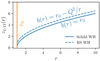 |
Fig. 1. Wormhole embedding functions zI and zII for both Schwarzschild and RN wormhole models, with r0 = 1, M = 0.5, and Q = 0.1. |
3. Test particle orbital motion
In this section we present the formalism of orbital mechanics within the general theory of relativity and probe the movement of test particles around the exotic wormhole geometries that we consider. Because the metric tensor depends only on r and θ (in our case, because of the spherical symmetry, theta is fixed to a π/2 equatorial slice), there are two Killing vectors, ξt = ∂t and ξϕ = ∂ϕ, which can be translated into conserved quantities (Águila & Matos 2018):
 (15)
(15)
![Mathematical equation: $$ \begin{aligned}&\ddot{r}=\frac{1}{2g_{rr}}\bigg [\partial _r g_{tt}\dot{t}^2+\partial _r g_{rr}\dot{r}^2+\partial _r g_{\phi \phi }\dot{\phi }^2\bigg ] \end{aligned} $$](/articles/aa/full_html/2022/09/aa44358-22/aa44358-22-eq17.gif) (16)
(16)
 (17)
(17)
Here, as usual, ℰ and ℒ respectively denote the conserved quantities, namely the energy and angular momentum of the test particle (time-like or null-like). For the time-like geodesics satisfying the ds2 = −m2 equation, the particle’s energy can be rewritten in the more suitable form
 (18)
(18)
where Veff is the effective potential of a gravitational field around a supermassive object. For generalized space-time, the effective potential reads (Karimov et al. 2019)
 (19)
(19)
3.1. Stable circular orbits
Now we can discuss the different kinds of orbits present in orbital dynamics. Stable circular orbits in the equatorial plane can be obtained by imposing  and
and  . By plugging these conditions into Eq. (18), we obtain that Veff = dVeff/dr = 0 and that d2Veff/dr2 < 0. These conditions imply the special values of conserved quantities, such that
 (20)
(20)
 (21)
(21)
In order to respect the equality dVeff/dr, Ω must also be constrained (Rahaman et al. 2021):
 (22)
(22)
3.2. Photon sphere
On the other hand, there are very different requirements for the photon sphere:
 (23)
(23)
Therefore, with the help of the expression for the proper distance, ds2 = 0, we get
 (24)
(24)
where for null-like geodesics, the effective potential reads (Godani & Samanta 2021)
 (25)
(25)
It is interesting that, judging by Eq. (24), the wormhole throat can act as a photon sphere by itself, since b(r0) = r0, and, because of this throat condition, ṙ = 0 automatically holds at r = r0. On the other hand, we can plot the light ray trajectories using Eqs. (16) and (17):
 (26)
(26)
Applying the appropriate change of coordinates, r → 1/u, we get
 (27)
(27)
Equation (27) can be solved numerically in polar coordinates (r, ϕ) for the special forms of both Φ(r) and b(r).
3.3. Model I
Now we compute the quantities for Eqs. (20)–(22) for the first wormhole model, namely the Schwarzschild-like wormhole with a constant shape function:
 (28)
(28)
 (29)
(29)
 (30)
(30)
We plot the normalized effective potential for a Schwarzschild-like wormhole with varying free parameter α in Fig. 2. We mark the potential of the photon sphere and its derivatives; the photon sphere is located at rph, where the effective potential has its maximum Veff(rph) = ℰ2, its first derivative vanishes, and the second-order radial derivative is negative. Also, after solving four-dimensional geodesic equations, we plot the null-geodesics with different values of impact parameter b = |ℒ|/ℰ in the left panel of Fig. 3.
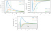 |
Fig. 2. Normalized effective potential and its radial derivatives for a Schwarzschild-like wormhole with a varying α parameter. |
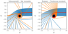 |
Fig. 3. Orbits of null-like particles around Schwarzschild-like and RN wormholes with α = 2, Q = Λ = 0.1, and M = 0.5. Here, blue trajectories are direct, red trajectories are photons, and orange trajectories are reconstructed with the help of lensing. |
3.4. Model II
Following the same procedure as done for the Schwarzschild-like wormhole, now we derive the conserved quantities for the traversable wormhole sourced by the electromagnetic field:
 (31)
(31)
 (32)
(32)
 (33)
(33)
In order to investigate the effective potential, normalized by L2, we want to numerically solve Eq. (25). The results of such an investigation are plotted in Fig. 4. We assume both a DS wormhole (a specific case of an RN wormhole with a vanishing charge) and a regular RN wormhole. It is obvious that for each case (DS and RN) a photon sphere exists, which is validated by the effective potential peak near the throat and its radial derivatives. Additionally, following the same procedure that was applied for the Schwarzschild wormhole, we show the null-like trajectories near the charged wormhole solution in the right panel of Fig. 3.
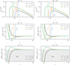 |
Fig. 4. Normalized effective potential and its radial derivatives for an RN wormhole with a varying electromagnetic charge, Q, and Λ parameter. |
4. Thin accretion disks and their optical properties
In the following we briefly discuss the physical properties of optically thick accretion disks. Such accretion disks occur near compact objects (both of singular and nonsingular nature) because of the mass transfer onto the massive object. Because of the present matter viscosity (both shear and bulk), matter falls onto the compact object – in the case of the black-hole solution, onto the event horizon; on the other hand, if one assumes a wormhole to be a compact object, matter transits through the wormhole throat into the other universe. It is obvious that for thin accretion disks, matter content is generally distributed within the equatorial plane. As mentioned in Rahaman et al. (2021), thin accretion disks in ray-tracing simulations inhabited by null-like particles with four-velocity Uμ form a photon sphere near the wormhole throat and have an averaged surface density of
 (34)
(34)
Here, H denotes the accretion disk height, such that H/R ≪ 1, and ⟨ρ0⟩ denotes the averaged energy density assuming θ = 2π. Here, we used the following definition of an energy-momentum tensor for the imperfect fluid (since the energy flux is present, non-diagonal components could be nonzero; Misner et al. 1973):
 (35)
(35)
As usual, in Eq. (35) η and ζ are shear and bulk viscosities, respectively, θ = ∇μUμ, qμ is the energy flux vector, tμν is the stress tensor, hμν is the induced metric, and h is its trace:
 (36)
(36)
Finally, we can also give the definition for the shear tensor:
 (37)
(37)
If the entropy for the considered fluid is conserved and shear and bulk viscosities are omitted, Eq. (35) can be greatly simplified to
 (38)
(38)
(the isotropic pressure vanishes as well). This is exactly the energy-momentum tensor for the perfect fluid with the present energy flow and stress. In addition to the averaged surface density, one can also compute radiation flux and disk torque for the sake of completeness (Rahaman et al. 2021):
 (39)
(39)
 (40)
(40)
Here,  denotes the averaged off-diagonal component of the stress tensor. Finally, combining everything (with the use of an energy-momentum tensor and the baryon conservation equations), we obtain the exact expression of the radiation flux, the most fundamental quantity of thin accretion disks (Thorne 1974; Rahaman et al. 2021):
 (41)
(41)
 (42)
(42)
where Ṁ is the mass accretion rate, which in our case is constant, and rms is the radius of the marginally stable orbit, which for Schwarzschild and RN wormholes equals
 (43)
(43)
 (44)
(44)
Several additional quantities can be computed, such as the thin accretion disk temperature (Torres 2002):
 (45)
(45)
where σ is the usual Boltzmann constant; here we assume that it equals unity for the sake of simplicity. Therefore, we numerically solved Eqs. (41) and (45) with the use of a numerical integrator for Schwarzschild and RN wormholes and for a Schwarzschild black hole in order to compare the results. To produce the plots, we, as usual, assume that the Schwarzschild-like wormhole radius is unitary, RN M = 0.5, and charge Q = 0.1. Moreover, the DS parameter Λ = 0.1. For the Schwarzschild black hole, we used the same mass, M = 0.5, that was used for both RN and Schwarzschild-like wormholes. Results for the radiation flux and the black-body temperature are given in arbitrary units in Fig. 5. Now we briefly discuss the results for each space-time kind.
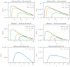 |
Fig. 5. Radiation flux and temperature for Schwarzschild-like wormholes, RN wormholes, and Schwarzschild black holes for comparison, with σ = 1, Q = Λ = 0.1, M = 0.5, r0 = 1 (for the Schwarzschild wormhole), and Ṁ = 10−12 M yr−1. |
Schwarzschild wormhole: this is the first wormhole model we consider. For this solution, one can easily notice that the radiation flux maximum shifts to r → ∞ if we assume relatively large values of the α parameter, which coincides well with the effective potential from Fig. 2. The same behavior can be observed for the black-body temperature.
Reissner-Nordström wormhole: this is the second (and final) exotic wormhole space-time that we examine. For this case, it is obvious that maxF(r)→0 as Λ → ∞. Therefore, similar to the Schwarzschild wormhole, the radiation flux of the thin accretion disk matches the Veff. However, we note that both the radiation flux and the temperature have smaller values in relation to the first wormhole model.
Schwarzschild black hole: this is the simplest black hole model with spherical symmetry; it is added for comparison. For the SS (spherically symmetric) black-hole solution, we note that, generally, the radiation, flux F(r), and the black-body temperature of the accretion disk, T(r), are smaller than those derived for our wormhole models (however, the results match with the RN wormhole for the vanishing DS parameter and the electromagnetic charge, as expected).
Since we have already investigated all of the necessary thin accretion disk properties numerically and graphically, we next obtained the images of these accretion disks near our two wormhole models with the use of ray-tracing techniques, as explained in detail, for example, in the pioneering works of Paul et al. (2020) and Shaikh & Joshi (2019). In order to obtain the images, we modified the open-source ray-tracing code GYOTO (this code was described in Vincent et al. 2011, 20161). Images were obtained from the point of view of the asymptotically far located observer; we assume that the observer plane lies within θ = π/2 (equatorial region) and that robs = 500r0. Additionally, as seen from the value of robs, we assume only the case where the asymptotical observer is located in the same universe as the accretion disk; such an assumption has been made for the sake of GYOTO output validity.
4.1. Model I
We plot the ray-tracing images of the accreting torus (which is optically thin) for Schwarzschild-like wormholes with the varying (and positive) values of α in Fig. 6. To produce these images, we used inclination angles i = 105° and i = 20°. The latter was chosen to produce the images in which black-hole and disk spin vectors are directed "into the page" (for more details on the subject, see Walker et al. 2018; Akiyama et al. 2019c; Vincent et al. 2021). Now we investigate each image of the Schwarzschild wormhole.
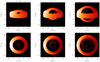 |
Fig. 6. Ray-tracing simulations of an accreting optically thin torus around the Schwarzschild-like wormhole with varying α. |
First case: α = 0. This case refers to the vanishing redshift function, and therefore a zero tidal forces (ZTF) wormhole, since, for our spherically symmetric line element, the redshift function acts as a gravitational potential. As already depicted in Fig. 2, the radius of the photon sphere (which is defined as a last stable orbit, formed by null-like particles, that often acts as the inner radius of an accretion disk near the compact objects) decreases as α → 0; this can be seen in the first and fourth panels of Fig. 6. From the ray-tracing simulations, we conclude that the photon sphere exists for the case with vanishing tidal forces; however, it could be completely indistinguishable if we assume the EHT resolution (which equals approximately ≈20 μas, as reported by Event Horizon Telescope Collaboration 2019). In this figure we can easily identify the light ring (i.e., the photon sphere) and a thick annular area (as seen from the polar region). The thick annular region corresponds to the optically thin accreting tori.
Second case: α = 1. As the second case, we considered the redshift function Φ = −1/r, which corresponds to the value of α = 1. Here, the redshift function does not vanish, but, because of the asymptotical flatness condition, Φ → 0 as r → ∞, as required for the viability of the theory. For the second case, as for the previous one, the photon sphere can be recognized by the asymptotically far zero angular momentum observer (ZAMO) as well as the thick annular area (polar projection of the thin accretion disk with a toroidal nature). Additionally, for unblurred images one can notice that a secondary, faint ring appears near the photon sphere, which may be a product of lensing. However, the secondary ring unfortunately cannot be observed by the current VLBI interferometers, but it could be in the future (for example, using the extended EHT2025 configuration).
Third case: α = 2. The last value of α that we consider in the present study is α = 2, for which the redshift function has exactly the form Φ = −2/r. In the previous subsections we investigated the Schwarzschild wormhole orbital mechanics with the help of the effective potential, Veff (for a more detailed graphical representation, see Fig. 2). This third case has rph = 2r0ℒ2, which is validated by the ray-tracing simulations in the third and sixth panels of Fig. 6. For α = 2 and larger values of α, a secondary light ring can be recognized more easily since its radius grows as α → ∞. Moreover, the inner radius of accreting tori grows with increasing α.
Now that we have discussed all three cases for a Schwarzschild wormhole, we can move on to our second wormhole model, namely the RN wormhole. In the following subsection, we investigate both RN wormholes with a positive charge and a special case, namely a DS wormhole with a vanishing electromagnetic charge.
4.2. Model II
The results of the ray-tracing near the RN wormhole are plotted in Fig. 7 with the different values for the Λ parameter and inclination; we have chosen two cases, with i = 105° and i = 20°. This choice of inclination was discussed in the previous subsection. Consequently, following the same procedure that was applied for the Schwarzschild wormholes, we now discuss the ray-tracing images produced for Λ = 10−3, 10−2, and 10−1.
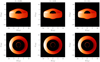 |
Fig. 7. Ray-tracing simulations of an accreting optically thin torus around a charged RN wormhole with Q = 0.1, M = 0.5, and a varying Λ. |
First case: Λ = 0.001. For this option, RN wormhole tidal forces are the smallest of the choices of Λ in our paper. Moreover, the gravitational potential, Φ, vanishes at asymptotical infinity and satisfies both conditions of asymptotical flatness and lack of horizon. Consequently, as prescribed by the effective potential and its derivatives from Fig. 4, the radius of the photon sphere, rph, is the biggest and shrinks as Λ → ∞. For a vanishing Λ, rph coincides with the RN black hole case. Moreover, for the relatively small and positive values of the Λ parameter, a secondary lensed light ring appears near the photon sphere.
Second case: Λ = 0.01. This is the second case we consider for RN-like wormholes. Now our wormhole solution differs from the RN black hole more, which is confirmed by the smaller radius of the photon sphere. However, a secondary lensed ring can still be observed. For the EHT resolution of 20 μas, a secondary ring will be absorbed into the main photon ring because of the big difference in flux.
Third case: Λ = 0.1. This is the last case under consideration. It has the smallest-radius photon sphere among the chosen values of Λ. Therefore, tidal forces of such a wormhole solution are the largest, which could be the answer as to why the photon ring shifts up to the wormhole throat. Remarkably, for Λ ≫ 0, one can observe the secondary lensed ring disappear.
Every feature of the ray-tracing images mentioned above holds for the special case with vanishing electromagnetic charge (the DS wormhole), except that the radius of the photon ring for each case is slightly smaller.
We have discussed each case for both Schwarzschild-like and RN wormholes. We now investigate the geometrically thick accretion disks and process the obtained images in order to achieve the EHT VLBI resolution (20 μas).
5. Thick disk and EHT imaging
Here we study the geometrically thick (optically thin) accretion disks around the exotic wormhole models that we consider. In the GYOTO package, thick accretion disks are generally parameterized by two fundamental quantities, namely the disk inner radius (in our paper, we set rin = r0 in order to reproduce the physically viable case) and disk opening angle, θop, which defines the angle between the equatorial plane, θ = π/2, and the accretion disk surface (it is worth noting that there is no outer disk radius implemented, since it depends on the chosen spectrograph maximal radial coordinate value, rmax). As emphasized in Vincent et al. (2021), to produce optically thin ray-tracing images of an accretion disk, one must assume that θop = 30°. In the open source package GYOTO, one can also assume the magnetization of the accretion disk with the help of the magnetization parameter σ = ℬ2/4π/(mpc2ne); here ℬ is the magnetic field amplitude, mp the proton mass, and ne the electron number density. We used the value of magnetization parameter σ = 0.01, which is set by default in the GYOTO package. We also fixed the electron number density and the accretion disk temperature at the inner radius to ne(rin) = 2.4 × 105 cm−3 and T(rin) = 8 × 10¹⁰ K, respectively. Finally, we used the following expression for the accretion flow four-velocity (measured by the ZAMO),
 (46)
(46)
so that both time-like and Vϕ four-velocity components vanish. To favor a circularly rotating accreting flow, one must assume purely azimuthal velocity, and therefore
 (47)
(47)
where
 (48)
(48)
One can also produce a ray-tracing image of the radially plunging flow if Uϕ = 0.
5.1. Model I
As usual, we start our investigation with the first wormhole solution, namely a Schwarzschild-like wormhole with a varying gravitational potential, Φ. Contrary to the thin accreting torus case, here we only consider one value of inclination, i = 20°. Such a value can provide complete information about the wormhole configuration (radius of the photon sphere and secondary ring). Additionally, our image coincides with the EHT VLBI network point of view. All of the images, which are listed below, were obtained in the EHT band ν = 230 GHz. Moreover, in order to reproduce the images blurred up to the EHT resolution, we used the package ehtim (for a detailed description of the package and its capabilities, see Chael et al. 2016, 20182). The key points for each case (α = 0, 1, 2) are as follows.
First case: α = 0. The vanishing α corresponds to the ZTF Schwarzschild wormhole. Only for the ZTF case can one notice the well-defined boost toward the observer, which arises because of the special relativistic effects and the Doppler shift: accretion flow with a circular rotation coming toward the observer causes the anisotropic distribution of the flux density within the thick accretion disk, which is in agreement with the EHT observations. Additionally, the aforementioned boost is present for the nonvanishing tidal forces, but not as strong as for the ZTF case.
First case: α = 1. For non-ZTF cases, a photon ring can be easily differentiated from the thick accretion disk even at the EHT resolution. As expected, the photon ring has a greater angular diameter, but a secondary ring could not be resolved.
First case: α = 2. This is the last value of α that we use to probe the thick accretion disk. In this case we observe that a secondary ring appears. As one can see, now the photon ring completely decouples from the thick accretion disk, but the secondary ring is absorbed by the photon ring in the blurred image with low resolution. We can approximately constrain the values of α to be relatively small and positive, since it was reported by the EHT collaboration that asymmetric ring-like structures were observed at the radius of 40 μas (Akiyama et al. 2019c). General relativity magnetohydrodynamic (GRMHD) simulations of various wormhole models show that this ring-like feature may be the well-known photon ring and that its asymmetry is caused by the black hole spin (Akiyama et al. 2019c).
5.2. Model II
The second wormhole model is, as before, a spherically symmetric wormhole that preserves electromagnetic charge. Ray-tracing simulation snapshots for this wormhole model are presented in Fig. 8. The radius of the photon ring decreases with increasing values of Λ (which is a difference between our wormhole model and the RN charged black hole). As already mentioned, the EHT has observed a ring-like feature with an angular diameter of approximately 40 μas. This could lead, for our model, to the relatively large and positive values of Λ needed for the model to match VLBI observations.
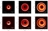 |
Fig. 8. Ray-tracing images of the RN wormhole surrounded by thick accretion disk polar regions with Q = 0.1 and a varying DS parameter, Λ, and rotating accretion flow (vϕ = 1). Using contours, we also depict plunging accretion flows (vϕ = 0). |
5.3. Radially plunging flow
Here, in contrast to the previous subsections, we assume a radially plunging flow that is defined by vϕ = Vϕ/V = 0 such that Vϕ vanishes.
Contours of ray-tracing simulation snapshots with vanishing azimuthal velocity are shown in Figs. 9 and 8 for both Schwarzschild and RN wormholes for the sake of comparison between the vϕ = 1 and vϕ = 0 cases. As we see, the pictures of radially plunging accretion flows do not deviate significantly from the ones with rotating matter content (Vr = Vϕ ≠ 0).
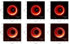 |
Fig. 9. Ray-tracing images of the Schwarzschild-like wormhole surrounded by thick accretion disk polar regions with a varying α. Here we depict both rotating and radially plunging flows (with the use of contours). |
6. Imaging accretion jet
Astrophysical compact objects are often associated with collimated, relativistic jets of matter expelling from the objects close to the speed of light. These jets are associated with strong magnetic fields whose underlying GRMHD physics provides insights into the dynamics of the accretion disk, associated compact object, stellar progenitor, and the object environment. This is relevant for studies associated with SMBHs and active galactic nuclei and help in understanding galaxy and stellar evolution since they have been shown to affect star formation rates, aiding and constraining star formation by supplying energy to the surrounding interstellar medium (Mizuno 2022; Ressler et al. 2021). The formation and destruction of these jets is an active area of study with the goal of understanding astrophysical turbulence and objects such as neutron stars and X-ray binaries. This is, however, beyond the scope of the current work; further information is available in Ressler et al. (2021) and Kylafis et al. (2012).
Ray-traced images of black holes, wormholes, and other compact objects, similar to the ones we have obtained thus far, show features across a large range of length scales. These range from extremely fine structures observed in accretion tori and photon rings to large-scale coherent structures observed in the relativistic jets associated with such objects. In this section we focus on imaging and observing the latter by analyzing ray-traced images of jet-thick accretion disk systems around exotic wormhole models. This is somewhat similar to what was done by Kramer & MacDonald (2021), who used radioactive transfer calculations on three-dimensional GRMHD simulations to understand jet dynamics. We extend their methods to study jets associated with thick-disk exotic wormholes. These jets are generally found to coexist with optically thick accretion disks, commonly observed in SMBHs found at galaxy centers, some white dwarfs, and neutron stars, and they have been hypothesized to exist with wormholes as well (Kirillov & Savelova 2020).
In this section we construct the model of a thick accretion disk with a jet in order to obtain the ray-tracing image, similar to M87. We introduce the physical properties of the simple analytical jet model, which is discussed in detail in the pioneering works of Móscibrodzka & Falcke (2013) and Davelaar et al. (2018). In these papers, GRMHD simulations of accretion relativistic jets were set up, and it was unveiled that the inner parts of the jet (the so-called spine) generally do not contain emitting matter and that emission therefore comes only from the outer jet regions (the jet sheath).
Within the GYOTO disk-jet model, there is a large variety of free parameters, which define the jet accretion properties present at the moment. For example, the emitting region of the jet is defined by two angles, θ1 and θ2. Since this emission layer is assumed to be thin, θ2 is only slightly bigger than θ1. Moreover, there is the so-called jet base height, zb. Following the work of Vincent et al. (2019), we set θ1 = θ2 − 3.5 = 20° and the jet base height equal to the wormhole throat radius, zb = r0. Moreover, we assume that the bulk Lorentz factor measured by ZAMO is Γ = 1.15 (which is set by default in the simulation suite). In order to properly ray-trace our exotic wormhole space-times, we need to define the exact form of the jet particles’ four-velocity (Vincent et al. 2019):
 (49)
(49)
Here UZAMO is the four-velocity of the observer with vanishing angular momentum that is located at the asymptotically flat region and V is the velocity of the relativistic jet measured by ZAMO (with vanishing time-time and ϕϕ components). This velocity has only two nonvanishing components (namely radial and θθ) because of the relativistic jet axial symmetry and stationary nature. It is more appropriate to write the jet velocity and its nonvanishing components in terms of sheath angles θ1 and θ2:
 (50)
(50)
where er and ez are, respectively, radial and azimuthal unit vectors and  is the jet velocity given in the units of light speed. In the equation above, θk could be equal to both the inner and outer opening angles. Next we investigate the structures that appear around exotic traversable wormholes.
6.1. Model I
The first traversable wormhole model we discuss is, as before, the Schwarzschild-like wormhole with nonvanishing gravitational potential. Numerical results are represented in Fig. 10 with varying values of the free parameter α (i.e., varying tidal force strength). Firstly, we discuss the vanishing α case.
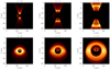 |
Fig. 10. Ray-tracing simulations of an accreting optically thick disk with a relativistic jet around a tidal Schwarzschild-like wormhole with r0 = 1 and a varying α. |
ZTF wormhole: as already observed, for the ZTF traversable wormhole solution with a constant shape function, the photon sphere has the smallest radii (and therefore the accretion disk rin ≈ rph is relatively small). These accretion disk features were seen in the ray-tracing image for the disk-jet system as well. However, here we also see that the actual size of the relativistic jet is smaller in relation to the other cases with α > 0, which is expected.
α = 1, 2 case: on the other hand, for the nonvanishing gravitational potential Φ(r) = − 1/r (or Φ(r) = − 2/r), the accretion disk becomes fainter in relation to the relativistic jet brightness. As previously noted, the angular diameter of the jet grows with the photon sphere radius. Moreover, for inclination angle i = 70°, the photon sphere is easily noticed, even with the EHT resolution.
In all of the cases, the brightness of the relativistic jet dominates over the accretion disk luminosity. However, it can be fixed with the assumption of a higher inner disk temperature, Tin. There is also the brightest area of the relativistic jet, located near its base, which is able to appear because of the photon bending; its radius approximately equals the radius of the photon sphere.
6.2. Model II
Our second and last wormhole model is the charged RN wormhole. Ray-tracing images of the relativistic jet and accretion disks for RN wormholes are shown in Fig. 11. The photon sphere and relativistic jet get slightly smaller as Λ → ∞, and the disk and relativistic jet become fainter with growing DS parameter values.
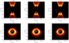 |
Fig. 11. Ray-tracing simulations of an accreting optically thick disk with a relativistic jet around a tidal RN wormhole with M = 0.5, Q = 0.1, and a varying Λ. |
7. Microlensing of the star bulb
The last ray-tracing scenario we study is the microlensing of the star bulb (radiative fluid sphere), caused by the wormhole curvature. In order to produce the ray-tracing images, we used the GYOTO fixed star scenario and placed the star bulb at rst = 10r0 assuming that the star radius is R = 4 (for a Schwarzschild-like wormhole) or R = 6 (for an RN wormhole). With the help of microlensing, one can see how the wormhole shadow changes with changing α and Λ values. We also varied the value of ϕ for a fixed star from ϕ = π up to ϕ = π/2.
7.1. Model I
The main feature to determine for the Schwarzschild wormhole is the radius of the wormhole shadow. Approximate values of the wormhole shadow radius, Rsh, for α = 0, 1, 2 are plotted in Fig. 12. We see that the radius of the wormhole shadow grows linearly with α, which is also validated by the linear regression that fits perfectly for the obtained data set (we also plot the 95% confidence intervals in the figure):
 (51)
(51)
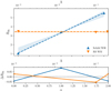 |
Fig. 12. Radius of the Schwarzschild-like (blue triangles) and RN (orange triangles) wormhole shadow with varying α (lower axis) and Λ (upper axis) with the present linear regression fits. |
7.2. Model II
Here we briefly discuss the RN wormhole shadows. It can generally be said that the radius of the RN wormhole shadow shrinks with the growing values of Λ, which coincide with the decreasing radius of the photon ring, as seen in Fig. 8. The linear regression fit for our data set is
 (52)
(52)
8. Concluding remarks
In this article we comprehensively investigate the accretion flows around two exotic wormholes with tidal forces present, namely a Schwarzschild-like wormhole with a constant shape function and an RN wormhole with an electromagnetic field respecting the U(1) local gauge symmetry (for the sake of completeness, we investigate both RN wormholes and a special case with vanishing electromagnetic charge, namely a DS wormhole). In order to examine the accretion flows around the spherically symmetric wormhole solutions, we used effective potential and ray-tracing methods, applied for both geometrically thin and geometrically thick accretion disks.
We used the effective potential normalized by ℒ2 to derive the radius of the photon sphere and observe its dynamics with the change of free parameters (additional degrees of freedom) α and Λ. For the Schwarzschild wormhole we considered both the ZTF case and the case with tidal forces. A detailed discussion of the test particle orbital mechanics and the derivation of Veff can be found in Sect. 3. A graphical representation of the Veff numerical solutions is given in Figs. 2 and 3. We also plot the particle orbits around both of our wormhole models, obtained with the help of lensing, direct ray-tracing, and photon ray-tracing, on Fig. 4.
We have also introduced thin accretion disks and their optical properties. We derived the radiation flux and temperature for Schwarzschild-like and RN wormholes and a Schwarzschild black hole surrounded by an optically thin accretion disk. We find that, generally, both the radiation flux and temperature of accretion disk endangered SS black hole which have the same mass as the wormhole solutions are smaller. Also, the behavior of the radiation flux and the temperature for both wormhole models coincide well with the effective potential. Numerical solutions, obtained with the help of Mathematica numerical integrator NIntegrate for F(r) and T(r), are shown in Fig. 5.
Finally, starting from Sect. 4.1, we used the numerous ray-tracing methods that were applied to our exotic wormhole models. Ray-tracing solutions for our analytical calculations give us images that can be compared against observations from the EHT and related surveys. These synthetic observations allow us to compare features between backgrounds of naked singularities, black holes, and wormholes, based on images of accretion disks with an associated photon sphere. We created these images based on numerical construction techniques developed in the open-source, massively parallel ray-tracing code GYOTO. These numerically constructed images allow us to qualitatively compare our models based on features found in the corresponding photon spheres and accretion tori, giving us further insight into the accretion behavior around these highly compact objects. In order to perform the ray-tracing for our studies, we modified GYOTO. All of the ray-tracing simulation snapshots were obtained on the Sharanga HPC (High Performance Computing) cluster nodes. Firstly, we used the optically thin accreting tori with an electromagnetic field and magnetization parameter σ = 0.01 as a ray-tracing scenario. We find that, for accreting tori, if we assume a Schwarzschild-like wormhole as a background massive and compact object, a photon sphere exists, even for the case with vanishing gravitational potential (however, with the EHT resolution of 20 μas, it may not be recognized). On the other hand, as predicted by the effective potential, the radius of the photon sphere shifts up to radial infinity if α → ∞ (see the ray-tracing images with varying α in Fig. 6). In the interest of accreting torus ray-tracing images around RN wormholes, we fixed the electromagnetic charge to Q = 0.1 < M = 0.5 (which is the physically plausible choice). Therefore, we are left with only one free parameter, namely the DS parameter, Λ, which marks the difference between a charged wormhole and a Schwarzschild black hole. We vary the DS parameter, Λ, in Fig. 7. After a careful numerical examination of the obtained ray-tracing images, we conclude that the radius of the photon sphere shrinks slowly as Λ increases (as prescribed by the effective potential).
We also used the thick disks as a probe of accretion flows around the exotic tidal wormhole solutions. A detailed discussion on this subject is presented in Sect. 5. We modified the standard thick disk GYOTO scenario for our needs and set the inner radius of the thick accretion disk to rin = r0. Moreover, we kept the thick disk opening angle and the magnetization parameter as defaults, and therefore θop = 30° and σ = 0.01. The black-body disk temperature and the inner radius is T(rin) = 8 × 10¹⁰ K and the electron number density ne(rin) = 2.4 × 105 cm−3; furthermore, the velocity, vϕ, was adopted to be purely azimuthal (from this fact it follows that the accretion flow is circularly rotating). On top of the usual ray-tracing simulations, we blurred the images to the EHT resolution of 20 μas (simulations were also approximated to the EHT ones by setting the inclination angle to i = 20° and the observation band to ν = 230 GHz). Images with both regular and blurred resolution can be seen in Figs. 9 and 8 for Schwarzschild-like and RN wormholes, respectively. It is clear that, similar to the accreting tori, the Schwarzschild-like wormhole rph → ∞ as α → ∞ and rph → 0 as Λ → ∞. Keeping that in mind and considering that ring-like asymmetric structures were observed for the M87 SMBH by the EHT with the radius ≈40 μas, we constrain the values of α to be relatively small and positive and Λ to be relatively large and positive in order to respect the EHT observational data.
Within this work we also comprehensively investigated the nature of a relativistic jet+thin accretion disk system for two wormhole models. As revealed by the ray-tracing simulations of null rays, the actual size of the relativistic jet for Schwarzschild-like wormhole grows as α → ∞. In contrast, for an RN wormhole, the relativistic jet size reduces as Λ → ∞. We also noticed that, in both cases, the relativistic jet brightness dominates over the accretion disk brightness (which can be fixed if higher values of inner temperature,Tin, are used).
The last feature that we probed using the GYOTO open source software is the microlensing of the fixed star bulb (with a varying ϕ coordinate) by the curvature of the various exotic wormhole models. Via microlensing, we were able to determine the approximate wormhole shadow radius, shown in Fig. 12. The ZTF Schwarzschild wormhole shadow radius is located very close to the wormhole throat; it then grows linearly with α. Alternatively, the Rsh for the RN wormhole decreases with growing Λ, as expected by theoretical predictions.
There has been some research done within the field of ray-tracing for various black holes and other exotic objects. For example, in Vincent et al. (2021) both Kerr and non-Kerr compact objects, including boson stars and Lamy wormholes, were probed using GYOTO. For nonrotating black holes, Vincent et al. (2021) find that the photon sphere lies inside the accretion disk for rin = rISCO and outside for rin = rH. Since we considered the first case, our results coincide only for relatively small, positive α and |Λ|≪1. On the other hand, if a black hole has spin (it was assumed in Vincent et al. (2021) that the black-hole spin generally equals to a = 0.8M), even for the option with rin = rISCO, rph > rin. Therefore, for that case parameter space for our models is larger, a Schwarzschild-like wormhole could have tidal forces. The situation with boson stars and Lamy wormholes is more complicated. In the boson star ray-tracing images, no particular photon ring was observed, but EHT images of our nontidal Schwarzschild wormhole could match the one obtained for a boson star. However, a Lamy wormhole has a very nontrivial ray-tracing image and a photon ring lensed several times, but if we match some free parameters, low resolution EHT images will converge. In the remarkable work of Rahaman et al. (2021), ray-tracing images of Teo class wormholes with spin surrounded by a Keplerian disk were comprehensively probed. In that paper, numerical dependences of a marginally stable orbit radius, rms, were derived from the dimensionless spin parameter J/M2, while for our models the analytical solution for rms is located in Eqs. (43) and (44). From that dependence, with equal throat radii one could easily distinguish our wormhole models from the Teo wormholes, which could be useful in the discussion on the nature of some compact massive objects.
In addition to the accretion disk ray-tracing, torus-jet images were obtained in Vincent et al. (2019) for the single case of a Schwarzschild black hole. Generally, the relativistic jet for our wormhole models looks very similar to that produced by the curvature of Schwarzschild black-hole space-time, so only the previously discussed constraints on the accretion disk should be applied. Additionally, in this study we compared the radiation flux of a classical Schwarzschild black hole and our wormhole models. We investigated the features of tidal wormholes that could distinguish such wormhole solutions from classical black holes or other exotic objects in observing campaigns such as that of the EHT. We have not considered the accretion disk located in the other universe. We constrained parameters α and Λ in order for wormhole solutions to match current M87 shadow observations performed by the EHT collaboration. In relation to the previous results for various other black-hole and wormhole models, our models can be precisely matched to recent VLBI observations; in future campaigns, we could easily vary the radius of the photon ring and the angular size of the relativistic jet. Furthermore, the James Webb Space Telescope could observe lensing effects caused by supermassive compact objects. Moreover, because of the nonsingular nature of such objects, many cosmological problems that arise from central singularities could be omitted. However, as already noted in many previous papers, with the EHT resolution of 20 μas, one can fine-tune almost any particular model to the observational constraints. In order to better understand the nature of the supermassive object being observed, one needs to increase the resolution of the image.
For the second paper of this series, we are planning to observe the magnetohydrodynamic features of the wormhole models studied in the present work.
Documentation is provided at http://gyoto.obspm.fr
The open source package, which works on the basis of regularized maximum likelihood, can be downloaded via http://github.com/achael/eht-imaging
Acknowledgments
We want to thank the Thibaut Paumard for the fruitful discussion on the GYOTO package and the provided help, guidance. As well, we want to express our sincere gratitude to the Frederic Vincent for the assistance on the EHT synthetic image producing. The authors gratefully acknowledge the computing time provided on the high performance computing facility, Sharanga, at the Birla Institute of Technology and Science – Pilani, Hyderabad Campus. P.K.S. acknowledges National Board for Higher Mathematics (NBHM) under Department of Atomic Energy (DAE), Govt. of India for financial support to carry out the Research project No.: 02011/3/2022 NBHM(R.P.)/R&D II/2152 Dt.14.02.2022. We are very much grateful to the honorable referee and to the editor for the illuminating suggestions that have significantly improved our work in terms of research quality, and presentation.
References
- Abbott, B. P., Abbott, R., Abbott, T. D., et al. 2016a, Phys. Rev. Lett., 116, 061102 [Google Scholar]
- Abbott, B. P., Abbott, R., Abbott, T. D., et al. 2016b, Phys. Rev. Lett., 116, 221101 [NASA ADS] [CrossRef] [Google Scholar]
- Águila, J. C. D., & Matos, T. 2018, CQG, 36, 015018 [Google Scholar]
- Akiyama, K., Alberdi, A., Alef, W., et al. 2019a, ApJ, 875, L1 [NASA ADS] [CrossRef] [Google Scholar]
- Akiyama, K., Alberdi, A., Alef, W., et al. 2019b, ApJ, 875, L2 [NASA ADS] [CrossRef] [Google Scholar]
- Akiyama, K., Alberdi, A., Alef, W., et al. 2019c, ApJ, 875, L5 [NASA ADS] [CrossRef] [Google Scholar]
- Akiyama, K., Alberdi, A., Alef, W., et al. 2019d, ApJ, 875, L6 [NASA ADS] [CrossRef] [Google Scholar]
- Anchordoqui, L. A., Torres, D. F., Trobo, M. L., & Perez Bergliaffa, S. E. 1998, Phys. Rev. D, 57, 829 [NASA ADS] [CrossRef] [Google Scholar]
- Bhattacharyya, S., Thampan, A. V., & Bombaci, I. 2001, A&A, 372, 925 [NASA ADS] [CrossRef] [EDP Sciences] [Google Scholar]
- Bronnikov, K. A., & Grinyok, S. 2002, ArXiv e-prints [arXiv:gr-qc/0205131] [Google Scholar]
- Caceres, E., Kundu, A., Patra, A. K., & Shashi, S. 2020, JHEP, 02, 149 [CrossRef] [Google Scholar]
- Cardoso, V., & Pani, P. 2019, Liv. Rev. Rel., 22, 1 [NASA ADS] [CrossRef] [Google Scholar]
- Cataldo, M., Liempi, L., & Rodríguez, P. 2017, Eur. Phys. J. C, 77, 748 [NASA ADS] [CrossRef] [Google Scholar]
- Chael, A. A., Johnson, M. D., Narayan, R., et al. 2016, ApJ, 829, 11 [Google Scholar]
- Chael, A., Rowan, M., Narayan, R., Johnson, M., & Sironi, L. 2018, MNRAS, 478, 5209 [NASA ADS] [CrossRef] [Google Scholar]
- Davelaar, J., Moscibrodzka, M., Bronzwaer, T., & Falcke, H. 2018, A&A, 612, A34 [NASA ADS] [CrossRef] [EDP Sciences] [Google Scholar]
- Einstein, A., & Rosen, N. 1935, Phys. Rev., 48, 73 [NASA ADS] [CrossRef] [Google Scholar]
- Event Horizon Telescope Collaboration (Akiyama, K. et al.) 2019, ApJ, 875, L4 [Google Scholar]
- Flamm, L. 2015, Gen. Rel. Grav., 47, 72 [NASA ADS] [CrossRef] [Google Scholar]
- Fuller, R. W., & Wheeler, J. A. 1962, Phys. Rev., 128, 919 [NASA ADS] [CrossRef] [Google Scholar]
- Gao, P., Jafferis, D. L., & Wall, A. C. 2017, JHEP, 12, 151 [CrossRef] [Google Scholar]
- Godani, N., & Samanta, G. C. 2021, Ann. Phys., 429, 168460 [NASA ADS] [CrossRef] [Google Scholar]
- Guzmán, F. S. 2006, Phys. Rev. D, 73, 021501 [CrossRef] [Google Scholar]
- Gyulchev, G., Nedkova, P., Vetsov, T., & Yazadjiev, S. 2019, Phys. Rev. D, 100, 024055 [NASA ADS] [CrossRef] [Google Scholar]
- Gyulchev, G., Kunz, J., Nedkova, P., Vetsov, T., & Yazadjiev, S. 2020, Eur. Phys. J. C, 80, 1017 [NASA ADS] [CrossRef] [Google Scholar]
- Harko, T., Kovacs, Z., & Lobo, F. S. N. 2009, CQG, 26, 215006 [NASA ADS] [CrossRef] [Google Scholar]
- Harko, T., Lobo, F. S. N., Mak, M. K., & Sushkov, S. V. 2013, Phys. Rev. D, 87, 067504 [NASA ADS] [CrossRef] [Google Scholar]
- Jusufi, K., Banerjee, A., & Ghosh, S. 2020, Eur. Phys. J. C, 80, 698 [NASA ADS] [CrossRef] [Google Scholar]
- Jusufi, K. K. S., Azreg-Aïnou, M., et al. 2022, Eur. Phys. J. C, 82, 633 [NASA ADS] [CrossRef] [Google Scholar]
- Karimov, R., Izmailov, R., & Kanti Nandi, K. 2019, Eur. Phys. J. C, 79, 952 [NASA ADS] [CrossRef] [Google Scholar]
- Karimov, R. K., Izmailov, R. N., Potapov, A. A., & Nandi, K. K. 2020, Eur. Phys. J. C, 80, 1138 [NASA ADS] [CrossRef] [Google Scholar]
- Karimov, R. K., Izmailov, R. N., Potapov, A. A., & Nandi, K. K. 2022, Eur. Phys. J. C, 82, 239 [NASA ADS] [CrossRef] [Google Scholar]
- Kirillov, A., & Savelova, E. 2020, Eur. Phys. J. C, 80, 1 [CrossRef] [Google Scholar]
- Kovács, Z., & Harko, T. 2010, Phys. Rev. D, 82, 124047 [CrossRef] [Google Scholar]
- Kramer, J. A., & MacDonald, N. R. 2021, A&A, 656, A143 [NASA ADS] [CrossRef] [EDP Sciences] [Google Scholar]
- Kylafis, N., Contopoulos, I., Kazanas, D., & Christodoulou, D. 2012, A&A, 538, A5 [NASA ADS] [CrossRef] [EDP Sciences] [Google Scholar]
- Lemos, J. P. S., & Zaslavskii, O. B. 2008, Phys. Rev. D, 78, 024040 [NASA ADS] [CrossRef] [Google Scholar]
- Lin, F. L., Patel, A., & Pu, H. Y. 2022, ArXiv e-prints [arXiv:2202.13559] [Google Scholar]
- Liu, C., Yang, S., Wu, Q., & Zhu, T. 2022, JCAP, 02, 034 [CrossRef] [Google Scholar]
- Maldacena, J., & Qi, X. L. 2018, ArXiv e-prints [arXiv:1804.00491] [Google Scholar]
- Matyjasek, J. 2020, Phys. Rev. D, 102, 024082 [NASA ADS] [CrossRef] [Google Scholar]
- Mirzaev, T., Abdikamalov, A. B., Abdujabbarov, A. A., et al. 2022, ArXiv e-prints [arXiv:2202.02122] [Google Scholar]
- Misner, C. W., Thorne, K. S., & Wheeler, J. A. 1973, Gravitation (San Francisco: W. H. Freeman) [Google Scholar]
- Mizuno, Y. 2022, Universe, 8, 85 [NASA ADS] [CrossRef] [Google Scholar]
- Moraes, P. H. R. S., Sahoo, P. K., Kulkarni, S. S., & Agarwal, S. 2019, Chin. Phys. Lett., 36, 120401 [NASA ADS] [CrossRef] [Google Scholar]
- Morris, M. S., & Thorne, K. S. 1988, Am. J. Phys., 56, 395 [NASA ADS] [CrossRef] [Google Scholar]
- Móscibrodzka, M., & Falcke, H. 2013, A&A, 559, L3 [NASA ADS] [CrossRef] [EDP Sciences] [Google Scholar]
- Nampalliwar, S., & Bambi, C. 2020, Tutorial Guide to X-ray and Gamma-ray Astronomy (Springer Singapore), 15 [CrossRef] [Google Scholar]
- Novikov, I. D., & Thorne, K. S. 1973, Black Holes (Les Astres Occlus), 343 [Google Scholar]
- Page, D. N., & Thorne, K. S. 1974, ApJ, 191, 499 [NASA ADS] [CrossRef] [Google Scholar]
- Paul, S., Shaikh, R., Banerjee, P., & Sarkar, T. 2020, JCAP, 2020, 055 [CrossRef] [Google Scholar]
- Rahaman, F., Manna, T., Shaikh, R., et al. 2021, Nucl. Phys. B, 972, 115548 [CrossRef] [Google Scholar]
- Ressler, S. M., Quataert, E., White, C. J., & Blaes, O. 2021, MNRAS, 504, 6076 [NASA ADS] [CrossRef] [Google Scholar]
- Shaikh, R., & Joshi, P. S. 2019, JCAP, 2019, 064 [CrossRef] [Google Scholar]
- Shakura, N. I., & Sunyaev, R. A. 1973, A&A, 24, 337 [NASA ADS] [Google Scholar]
- Thorne, K. S. 1974, ApJ, 191, 507 [Google Scholar]
- Torres, D. F. 2002, Nucl. Phys. B, 626, 377 [NASA ADS] [CrossRef] [Google Scholar]
- Vincent, F. H., Paumard, T., Gourgoulhon, E., & Perrin, G. 2011, CQG, 28, 225011 [NASA ADS] [CrossRef] [Google Scholar]
- Vincent, F. H., Meliani, Z., Grandclément, P., Gourgoulhon, E., & Straub, O. 2016, CQG, 33, 105015 [NASA ADS] [CrossRef] [Google Scholar]
- Vincent, F. H., Abramowicz, M. A., Zdziarski, A. A., et al. 2019, A&A, 624, A52 [NASA ADS] [CrossRef] [EDP Sciences] [Google Scholar]
- Vincent, F. H., Wielgus, M., Abramowicz, M. A., et al. 2021, A&A, 646, A37 [NASA ADS] [CrossRef] [EDP Sciences] [Google Scholar]
- Visser, M. 1995, Lorentzian wormholes: From Einstein to Hawking (AIP Series in Computational and Applied Mathematical Physics) [Google Scholar]
- Walker, R. C., Hardee, P. E., Davies, F. B., Ly, C., & Junor, W. 2018, ApJ, 855, 128 [Google Scholar]
- Wang, M., Chen, S., Wang, J., & Jing, J. 2020, Eur. Phys. J. C, 80, 110 [NASA ADS] [CrossRef] [Google Scholar]
- Yuan, F., & Narayan, R. 2014, ARA&A, 52, 529 [NASA ADS] [CrossRef] [Google Scholar]
- Yuan, Y.-F., Narayan, R., & Rees, M. J. 2004, ApJ, 606, 1112 [NASA ADS] [CrossRef] [Google Scholar]
- Yusupova, R. M., Karimov, R. K., Izmailov, R. N., & Nandi, K. K. 2021, Universe, 7, 177 [NASA ADS] [CrossRef] [Google Scholar]
All Figures
|
Fig. 1. Wormhole embedding functions zI and zII for both Schwarzschild and RN wormhole models, with r0 = 1, M = 0.5, and Q = 0.1. |
| In the text | |
|
Fig. 2. Normalized effective potential and its radial derivatives for a Schwarzschild-like wormhole with a varying α parameter. |
| In the text | |
|
Fig. 3. Orbits of null-like particles around Schwarzschild-like and RN wormholes with α = 2, Q = Λ = 0.1, and M = 0.5. Here, blue trajectories are direct, red trajectories are photons, and orange trajectories are reconstructed with the help of lensing. |
| In the text | |
|
Fig. 4. Normalized effective potential and its radial derivatives for an RN wormhole with a varying electromagnetic charge, Q, and Λ parameter. |
| In the text | |
|
Fig. 5. Radiation flux and temperature for Schwarzschild-like wormholes, RN wormholes, and Schwarzschild black holes for comparison, with σ = 1, Q = Λ = 0.1, M = 0.5, r0 = 1 (for the Schwarzschild wormhole), and Ṁ = 10−12 M yr−1. |
| In the text | |
|
Fig. 6. Ray-tracing simulations of an accreting optically thin torus around the Schwarzschild-like wormhole with varying α. |
| In the text | |
|
Fig. 7. Ray-tracing simulations of an accreting optically thin torus around a charged RN wormhole with Q = 0.1, M = 0.5, and a varying Λ. |
| In the text | |
|
Fig. 8. Ray-tracing images of the RN wormhole surrounded by thick accretion disk polar regions with Q = 0.1 and a varying DS parameter, Λ, and rotating accretion flow (vϕ = 1). Using contours, we also depict plunging accretion flows (vϕ = 0). |
| In the text | |
|
Fig. 9. Ray-tracing images of the Schwarzschild-like wormhole surrounded by thick accretion disk polar regions with a varying α. Here we depict both rotating and radially plunging flows (with the use of contours). |
| In the text | |
|
Fig. 10. Ray-tracing simulations of an accreting optically thick disk with a relativistic jet around a tidal Schwarzschild-like wormhole with r0 = 1 and a varying α. |
| In the text | |
|
Fig. 11. Ray-tracing simulations of an accreting optically thick disk with a relativistic jet around a tidal RN wormhole with M = 0.5, Q = 0.1, and a varying Λ. |
| In the text | |
|
Fig. 12. Radius of the Schwarzschild-like (blue triangles) and RN (orange triangles) wormhole shadow with varying α (lower axis) and Λ (upper axis) with the present linear regression fits. |
| In the text | |
Current usage metrics show cumulative count of Article Views (full-text article views including HTML views, PDF and ePub downloads, according to the available data) and Abstracts Views on Vision4Press platform.
Data correspond to usage on the plateform after 2015. The current usage metrics is available 48-96 hours after online publication and is updated daily on week days.
Initial download of the metrics may take a while.