| Issue |
A&A
Volume 561, January 2014
|
|
|---|---|---|
| Article Number | A114 | |
| Number of page(s) | 12 | |
| Section | Interstellar and circumstellar matter | |
| DOI | https://doi.org/10.1051/0004-6361/201219945 | |
| Published online | 17 January 2014 | |
Potential multi-component structure of the debris disk around HIP 17439 revealed by Herschel/DUNES⋆
1 UJF-Grenoble 1/CNRS-INSU, Institut de Planétologie et d’Astrophysique de Grenoble (IPAG) UMR 5274, 38041 Grenoble, France
e-mail:
This email address is being protected from spambots. You need JavaScript enabled to view it.
2 Dpt. de Física Teórica, Facultad de Ciencias, Universidad Autónoma de Madrid, Cantoblanco, 28049 Madrid, Spain
3 Astrophysikalisches Institut und Universitätssternwarte, Friedrich-Schiller-Universität, Schillergäßchen 2-3, 07745 Jena, Germany
4 ESA-ESAC Gaia SOC., PO Box 78, 28691 Villanueva de la Cañada, Madrid, Spain
5 Instituto Nacional de Astrofísica, Óptica y Electrónica, Luis Enrique Erro 1, Sta. Ma. Tonantzintla, Puebla, Mexico
6 European Space Observatory, Alonso de Cordova 3107, Vitacura Casilla 19001, Santiago 19, Chile
7 Jet Propulsion Laboratory, California Institute of Technology, Pasadena, CA 91109, USA
8 NASA Goddard Space Flight Center, Exoplanets and Stellar Astrophysics, Code 667, Greenbelt, MD 20771, USA
9 Institut für Theoretische Physik und Astrophysik, Christian-Albrechts-Universität zu Kiel, Leibnizstraße 15, 24098 Kiel, Germany
10 Onsala Space Observatory, Chalmers University of Technology, 439 92 Onsala, Sweden
11 ESA Astrophysics & Fundamental Physics Missions Division, ESTEC/SRE-SA, Keplerlaan 1, 2201 AZ Noordwijk, The Netherlands
12 Observatoire de Paris, Section de Meudon, Laboratoire d’études spatiales et d’instrumentation en astrophysique, 5 place Jules Janssen, 92195 Meudon Cedex, France
13 Department of Physics and Astrophysics, Open University, Walton Hall, Milton Keynes MK7 6AA, UK
14 Rutherford Appleton Laboratory, Chilton OX11 0QX, UK
Received: 3 July 2012
Accepted: 18 November 2013
Abstract
Context. The dust observed in debris disks is produced through collisions of larger bodies left over from the planet/planetesimal formation process. Spatially resolving these disks permits to constrain their architecture and thus that of the underlying planetary/planetesimal system.
Aims. Our Herschel open time key program DUNES aims at detecting and characterizing debris disks around nearby, sun-like stars. In addition to the statistical analysis of the data, the detailed study of single objects through spatially resolving the disk and detailed modeling of the data is a main goal of the project.
Methods. We obtained the first observations spatially resolving the debris disk around the sun-like star HIP 17439 (HD 23484) using the instruments PACS and SPIRE on board the Herschel Space Observatory. Simultaneous multi-wavelength modeling of these data together with ancillary data from the literature is presented.
Results. A standard single component disk model fails to reproduce the major axis radial profiles at 70 μm, 100 μm, and 160 μm simultaneously. Moreover, the best-fit parameters derived from such a model suggest a very broad disk extending from few au up to few hundreds of au from the star with a nearly constant surface density which seems physically unlikely. However, the constraints from both the data and our limited theoretical investigation are not strong enough to completely rule out this model. An alternative, more plausible, and better fitting model of the system consists of two rings of dust at approx. 30 au and 90 au, respectively, while the constraints on the parameters of this model are weak due to its complexity and intrinsic degeneracies.
Conclusions. The disk is probably composed of at least two components with different spatial locations (but not necessarily detached), while a single, broad disk is possible, but less likely. The two spatially well-separated rings of dust in our best-fit model suggest the presence of at least one high mass planet or several low-mass planets clearing the region between the two rings from planetesimals and dust.
Key words: infrared: stars / circumstellar matter / stars: individual: HIP 17439
Herschel is an ESA space observatory with science instruments provided by European-led Principal Investigator consortia and with important participation from NASA.
New affiliation: European Southern Observatory, Alonso de Cordova 3107, Vitacura, Casilla 19001, Santiago, Chile
© ESO, 2014
1. Introduction
Circumstellar debris disks around main-sequence stars are most usually observed as excesses above the stellar photospheric emission at far-infrared wavelengths due to dust emission. The dust in these disks is thought to be produced by collisions of planetesimals left over from the planet formation process in the system (see Krivov 2010 for a recent review). In addition to the stellar gravity and radiation, the presence of planets in the system may significantly sculpt the distribution of the dust and planetesimals through their gravitational interaction (Dominik & Decin 2003; Kenyon & Bromley 2004; Wyatt 2008; Ertel et al. 2012b). This can result in different features of the disk such as clumpy structures and multiple rings depending on the configuration and history (e.g., migration) of the underlying planetary system (Wyatt 2008; Ertel et al. 2012b). Indeed, candidates for such complex architectures have been observed in several systems (e.g., ϵ Eridani: Backman et al. 2009; Fomalhaut: Acke et al. 2012).
HIP 17439 (HD 23484) is a sun-like (sp. type K2 V, Torres et al. 2006; Gray et al. 2006), nearby (d = 16.0 pc, van Leeuwen 2007) main-sequence star with an estimated age of 760 Myr (Maldonado et al. 2010). The first conclusive detection of far-infrared excess was reported by Koerner et al. (2010) based on Spitzer/MIPS observations. Earlier detections of the excess were ascribed to contamination by galactic cirrus (Moór et al. 2006; Silverstone 2000). In this paper, we present far-infrared Herschel (Pilbratt et al. 2010) PACS (Poglitsch et al. 2010) and SPIRE (Griffin et al. 2010; Swinyard et al. 2010) images of the debris disk obtained in the context of our Herschel open time key program DUNES (DUst around NEarby Stars, Eiroa et al. 2010, 2013). These data are complemented by a re-reduction of the available Spitzer data (MIPS and IRS) as well as by other data from the literature. We present simultaneous multi-wavelength modeling of the debris disk considering all available, relevant data in order to constrain the architecture of the dust and planetesimal disk beyond the possibilities of single data sets. This way, we put constraints on the underlying planetary/planetesimal system potentially responsible for the complex disk structure.
We present the available data in Sect. 2, including predictions of the stellar photospheric flux and a re-reduction of the Spitzer data being the most relevant, complementary data to the new Herschel observations. In this section, we also describe the new Herschel data summarizing the observations, the data reduction, results, and present a basic analysis of the Herschel images (image deconvolution and radial profile extraction). In Sect. 3, analytical, simultaneous model fitting to all available data is presented including a detailed interpretation of the results. A summary and conclusions are given in Sect. 4.
2. Observations and data analysis
In this section, we present the observational data of the HIP 17439 system. This includes the characterization of the host star and the fitting of a stellar photosphere model, a re-reduction of the available Spitzer data, as well as a detailed description of our new Herschel observations, and the subsequent data reduction and analysis. This work is done analogous to the whole survey sample. For more details on the general observing strategy and data reduction of the DUNES survey see Eiroa et al. (2013).
2.1. Stellar parameters and photosphere estimation
Table 1 provides fundamental stellar parameters of HIP 17439. The bolometric luminosity has been estimated from the absolute V magnitude and the bolometric correction from Flower (1996). Effective temperature, surface gravity and metallicity are mean values of spectroscopic estimates by Valenti & Fischer (2005) and Santos et al. (2004). The projected rotational velocity is taken from Torres et al. (2006). HIP 17439 is an active star with a Ca ii  index of − 4.534 (Gray et al. 2006). The observed ROSAT X-ray luminosity LX/Lbol, is also given. The age of the star estimated from the index (Mamajek & Hillenbrand 2008) is 0.8 Gyr while from the X-ray luminosity following Garcés et al. (2010) it is 0.9 Gyr. A recent estimate using evolutionary tracks gives 3.7 Gyr (Fernandes et al. 2011), although we note that isochrones are highly degenerate for stars located right on the main sequence and are very sensitive to metallicity (Holmberg et al. 2009). Thus, we favor the consistent values estimated from the X-ray luminosity and activity index. The mass of the star using the gravity and stellar radius is 0.63 M⊙, while Fernandes et al. (2011) obtain 0.83 M⊙.
The stellar photosphere contribution to the total flux was calculated from a synthetic stellar atmosphere model interpolated from the PHOENIX/Gaia grid (Brott & Hauschildt 2005). After a comparison of possible normalization methods (e.g. to all near-infrared data, WISE-only or the Spitzer/IRS spectrum) the stellar models were scaled to the combined near-infrared and WISE band 3 fluxes following Bertone et al. (2004), as being the optimum solution. WISE band 2 was omitted due to saturation and WISE band 4 is in a region of the spectral energy distribution (SED) already exhibiting excess emission in the Spitzer/IRS spectrum.
Physical properties of HIP 17439, cf. discussion in Sect. 2.1.
2.2. Spitzer observations and photometry
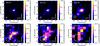 |
Fig. 1 Herschel/PACS and Herschel/SPIRE observations of HIP 17439. The band is noted in the upper left corner of each panel. The white circle in the lower left of each panel illustrates the FWHM of the theoretical, circular PSF. |
Our data analysis for the Spitzer/MIPS images (program ID: 30490, PI: Koerner et al. 2010) is similar to that described in Bryden et al. (2009). At 24 μm, images are created from the raw data using software developed by the MIPS instrument team (Gordon et al. 2005), with image flats chosen as a function of scan mirror position to correct for dust spots and with individual frames normalized to remove large scale gradients (Engelbracht et al. 2007). At 70 μm, images are also processed with the MIPS instrument team pipeline, including added corrections for time-dependent transients (Gordon et al. 2007). Aperture photometry at 24 μm and 70 μm is performed as in Beichman et al. (2005) with aperture radii of  and
and  , background annuli of
  and
and  , and aperture corrections of 1.15 and 1.79 at 24 μm and 70 μm, respectively. The 24 μm centroid positions, which are consistent with the telescope pointing accuracy of <1″ (Werner et al. 2004), are used as the target coordinates for both wavelengths. HIP 17439 is observed at 24 μm with high S/N; uncertainty at that wavelength is dominated by systematics at the level of ~2% for overall calibration and <1% for repeatability (Engelbracht et al. 2007). The 70 μm uncertainties are calculated from direct measurement of the sky background variation in each field, using the same apertures and corrections as for the photometry. A calibration uncertainty of 5% and a repeatability uncertainty of 4.5% (Gordon et al. 2007) are also included. The different contributions to the uncertainties are added quadratically. Color corrections of 1.12 and 0.893 at 24 μm and 70 μm, respectively, have been applied.
The Spitzer/IRS (Houck et al. 2004) spectrum of HIP 17439 (program ID: 50150, PI: Rieke) spans the two long wavelength, low resolution modules covering 14 μm − 40 μm. The spectrum presented here was taken from the CASSIS1 archive (Lebouteiller et al. 2011). Data are taken with the star at two locations along the slit to permit background subtraction. The final spectrum is the average of the two slit positions, whilst the uncertainty is estimated from the difference between the value at each wavelength. The slit width (~ ) is greater than the Spitzer pointing uncertainty of <1″, so flux loss outside the slit is minimal and no scaling of the individual modules is required (Werner et al. 2004). The CASSIS spectrum lies systematically above the model photosphere and we have therefore scaled the IRS spectrum by a factor of 0.93 to fit the predicted photosphere model at 14 μm. After scaling, fluxes in bands centered at 17 μm and 32 μm were calculated to look for evidence of warm excess and the rising excess from cold dust grains. The fluxes were measured in each band by summing the error-weighted fluxes of all points on the spectrum lying between 15 μm − 19 μm and 30 μm − 34 μm following Chen et al. (2006, 2007).
2.3. Herschel observations and photometry
HIP 17439 was observed with both PACS and SPIRE instruments. The resulting images at 70 μm to 500 μm are shown in Fig. 1 along with a circle illustrating the angular resolution of the observations (the full width at half maximum, FWHM, of the point spread function, PSF, assumed to be circular). We see no evidence of potential contamination from cirrus emission in the Herschel/PACS 70 μm image, confirming the circumstellar nature of the excess emission. Nearby background sources to the southeast and north become visible at 100 μm and 160 μm, but these can be clearly differentiated from the extended emission of the circumstellar disk in the PACS images presented in Fig. 1. In the SPIRE sub-mm images, measurement of the disk extent and source flux is complicated due to the decreasing source flux and the blending of the background sources with the disk due to the larger telescope beam size at those wavelengths.
Scan map observations of HIP 17439 were taken with both PACS 70/160 and 100/160 channel combinations. The observations were set up following the recommended parameters laid out in the scan map release note2, each scan map consisting of 10 legs of 3′, with a 4″ separation between legs, scanning at the medium slew speed (20″ per second). Each target was observed at two array orientation angles (70° and 110°) to improve noise suppression and assist in the removal of low frequency (1/f) noise, instrumental artifacts and glitches from the images by mosaicking. A SPIRE observation in small map mode3 was also taken of HIP 17439, producing a fully sampled map covering a region 4′ wide around the target. The Herschel observations are summarized in Table 2.
All data reduction is carried out in HIPE (Herschel Interactive Processing Environment, Ott 2010), using calibration version 45 for the data reduction and user release version 10 for the PACS data and calibration version 10 for the SPIRE data. The individual PACS scans are processed with a high-pass filter to remove 1/f noise, using high-pass filter widths of 15 frames at 70 μm, 20 frames at 100 μm and 25 frames at 160 μm, suppressing structures larger than 62″, 82″ and 102″ in the final images. For the filtering process, regions of the map where the pixel brightness exceeds a threshold defined as twice the standard deviation of the non-zero flux elements in the map are masked from the high-pass filter. De-glitching is carried out using the second level spatial deglitching task. The maps are created using the HIPE photProject task. The PACS scan pairs at 70 μm and 100 μm, and the four 160 μm scans (two each from PACS 70/160 and 100/160 observations) are mosaicked to produce the final images for each band. Final image scales are 1″ per pixel at 70 μm and 100 μm and 2″ per pixel at 160 μm, compared to native instrument pixel sizes of 3.2″ at 70 μm and 100 μm, and 6.4″ at 160 μm, respectively. For the SPIRE observations, the small maps are created using the standard pipeline routine in HIPE and the naïve mapper option. Image scales of 6″, 10″ and 14″ per pixel are used at 250 μm, 350 μm and 500 μm. The sky background and rms uncertainty is estimated from the mean and standard deviation of the total fluxes in 25 boxes of 7 × 7 pixels at 70 μm, 9 × 9 pixels 100 μm and 7 × 7 pixels at 160 μm placed randomly around the center of the image. The box sizes are chosen to match the size of a circular aperture with maximum signal-to-noise at each wavelength which was determined from an analysis adopted to point-like sources. Since our source is extended and the aperture size is much larger than that the boxes are tailored for, we scale the measured per pixel noise to reflect the larger aperture area used to measure the fluxes of HIP 17439. Regions are rejected if part of the box covers a region brighter than the threshold level as defined for the high-pass filtering and are spatially constrained to lie between 30″ and 60″ from the source position to avoid it and the lower coverage at larger distances from the center. The two nearby background sources are both fitted with a scaled and rotated (to account for the not perfectly circular shape of the telescope PSF with three side lobes the orientation of which depends on the telescope position angle during observations, here angle to be used is −103.4°) observation of α Boo as a point source model and subtracted from the images before flux measurement.
Summary of Herschel observations of HIP 17439.
The source flux in each of the three PACS images is measured using a circular aperture of radius 20″. The aperture radii are chosen to encompass the full extent of the disk at all three wavelengths. The measured PACS fluxes are corrected for the aperture radius following PICC-ME-TN-037 (their Table 15). Color correction is applied as a combination of two temperature components (the stellar photosphere and the dust) using an interpolated value of the appropriate correction from Table 1 in PICC-ME-TN-038 after fitting a black body to the dust thermal emission to gauge its temperature. Corrections applied are 1.016, 1.034, and 1.074 at 70 μm, 100 μm, and 160 μm, respectively, for the star (the contribution of the photosphere at SPIRE wavelengths is negligible), and 0.982, 0.985, 1.010, 0.9417, 0.9498, and 0.9395 at 70 μm, 100 μm, 160 μm, 250 μm, 350 μm, and 500 μm, respectively, for the disk. Raw values of the fluxes are 73.3 mJy, 90.0 mJy, and 92.8 mJy at 70 μm, 100 μm, and 160 μm, respectively, and 53.0 mJy, 32.2 mJy, and 12.7 mJy at 250 μm, 350 μm, and 500 μm, respectively. The PACS values are consistent with, but different from the ones in Eiroa et al. (2013), because they have been derived with another version of the pipeline (differces in calibration version, pointing reconstruction and mosaicking). While the version used in the present work is newer, the values in Eiroa et al. (2013) are consistently derived for all targets and thus to be preferred when studying the whole sample instead of modeling a single object. Using the values in Eiroa et al. (2013) for the fitting presented in the present work would not alter the results significantly, but would slightly increase their significance.
Optical and infrared photometry of HIP 17439.
At SPIRE wavelengths, the source is pointlike and the fluxes are measured in apertures of radii 22″, 30″, and 42″ at 250 μm, 350 μm, and 500 μm, with the sky background estimated from an annulus of 60″ − 90″ following the SPIRE aperture photometry recipe4. A summary of the optical and infrared photometry used in the SED fitting (including the new Spitzer and Herschel fluxes) is presented in Table 3. In the SPIRE images the background sources are modeled as Gaussians with the appropriate beam FWHM for the wavelength of observation and are also subtracted before flux measurement.
Uncertainties on the photometry have been computed as the quadratic sum of sky noise and calibration uncertainties (5% for PACS and 15% for SPIRE, see Eiroa et al. 2013 for details).
A full list of all photometric data of the HIP 17439 system considered is given in Table 3.
2.4. Observational results
We find the far-infrared emission to be associated with the star and interpret it as a circumstellar debris disk. The emission is extended compared to the PACS beam. From the SED we find that the emission is dominated by cold dust that must be located not too close to the star (significant emission starts between 24 μm and 32 μm, black body grains peaking at these wavelengths would be located at 1.35 au and 1.56 au from the star, respectively, which can be considered as a lower limit of the inner edge of the disk). We find no evidence for significant amounts of warm dust at few au from the star or less at the sensitivity of the available photometry. From a black body fit to the disk’s SED we find a temperature of 45.8 K and fractional luminosity Ldisk/Lstar = 10-4, which represent the first direct measurement of these values for the HIP 17439 disk (note the lower limit derived by Koerner et al. (2010) based on the Spitzer 70 μm flux only which is in good agreement with our value). In the following, we discuss the constraints that can already be put on the disk structure from the spatially resolved images. We will present deconvolved images of the debris disk as well as radial profiles that will be used later for model fitting.
2.4.1. Disk geometry and deconvolved images
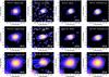 |
Fig. 2 Original images and deconvolved images at the three Herschel/PACS bands. Image type, wavelength and deconvolution method are noted in the upper left corner of each panel, respectively. The images are oriented north up, east left. Contours denote positive surface brightness values and are drawn in steps of 10% of the peak surface brightness. The color scale is linear and ranges from zero to the peak surface brightness. |
To derive a first estimate of the radial extent of the disk, its position angle, and its inclination, we fit a two dimensional Gaussian to the disk images at 70 μm, 100 μm, and 160 μm. In the images at SPIRE wavelengths, the disk is only marginally resolved (or not resolved at all). Thus, we do not consider these images. From the FWHM Aimage of the disk image at each wavelength measured along the major axis, we estimate the disk extent Adisk (the extent of the structure dominating the emission at each wavelength) through deconvolution using the following formula (convolving a Gaussian with another Gaussian): 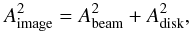 (1)where Abeam is the FWHM of the beam. While Adisk measured along the major axis of an image is representative of the diameter of the structure dominating the emission at this wavelength, the ratio between the deconvolved FWHM derived along the major axis, Adisk, and the minor axis, Bdisk (derived from the FWHM of the image along the minor axis, Bimage), gives an estimate of the disk inclination θ from face-on (assuming a geometrically thin, circular disk):
 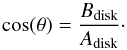 (2)Note that this inclination has to be considered as a lower limit due to the limited angular resolution of the observations. The results of this analysis are listed in Table 4.
Disk geometry measured from the PACS images.
Trying to resolve the dust depletion expected in the inner regions of the disk and in order to search for potential disk structures at the highest possible angular resolution, we perform image deconvolution on the PACS images. This deconvolution is a two-step process. Firstly, the stellar photosphere contribution is removed from each image by subtraction of a PSF rotated to the same position angle as the observations with a total flux scaled to the predicted photospheric level in that image centered on the stellar position determined from isophotal fitting of the 70 μm image. Secondly, after star subtraction, the image is deconvolved using an implementation of the van Cittert algorithm and the IRAF stsdas packages for modified Wiener and Richardson-Lucy deconvolution to check the suitability of the individual methods and the repeatability of any structure observed in the deconvolved images. The observation of α Boo adopted as a model PSF for the deconvolution process is assumed to be representative of a point source. However, analysis by Kennedy et al. (2012) have identified variations at the 10% level in the extent of the PSF FWHM at 70 μm for a variety of point source calibrators depending on the date and mode of observation (a smaller variation of 2–4% is seen at 100 μm). Variation at this level does not negate the interpretation of this target as an extended source, but should be kept in mind to avoid over interpretation of the extended structure revealed through the deconvolution process or of the results of the model fitting presented later, as the model images are concolved with the same PSF images in order to produce simulated observations. A comparison of the extent of the disk at different wavelengths in the PACS images is still valid, as the data have been obtained at the same day in the same observing mode.
A comparison of the three deconvolution methods used in this work is provided in Fig. 2. No significant structure or asymmetry is visible in these deconvolved images. Furthermore, despite the increased angular resolution, no dip or plateau of the surface brightness in the inner regions that would be indicative of an inner hole is visible. Thus, we conclude that the diameter of any depleted inner region of the disk is not significantly larger than the resolution reached after deconvolution (typically about a factor of two improvement over original resolution, i.e., approx. 50 au at 70 μm).
Furthermore, it becomes obvious that the extent of the disk measured at different wavelengths is significantly different according to both Eq. (1) and image deconvolution (a factor of two from 70 μm to 160 μm according to Eq. (1)). The possibility that this is caused by the lower angular resolution at longer wavelengths and imperfect deconvolution cannot be ignored. In contrast, in previous, similar data of HD 207129 (Löhne et al. 2012), we found for a disk with a confined, ring-like shape a good agreement between the extent measured at different wavelengths. Thus, we conclude that our present findings are indicative of a radially very extended disk with a shallow surface density profile (colder dust further away from the star emits more efficiently at longer wavelengths) or of a disk composed of multiple rings at significantly different radial distance from the star, and with flux ratios that vary significantly with wavelength in the Herschel/PACS spectral range. We will further discuss these scenarios in the modeling section.
2.4.2. Radial profiles
Radial profiles are useful to visualize extended emission. Furthermore, we use radial profiles in our simultaneous multi-wavelength fitting of the data presented later in this paper. We produce radial profiles of the source for each PACS wavelength in the following manner: a cutout of the mosaic image at each wavelength is centered on the stellar position and the disk position angle is determined by fitting a 2D Gaussian to the source brightness profile at 100 μm (same procedure as in the previous section). Each cutout is then rotated such that the disk major axis lies along the rotated image’s x-axis. The cutout is then interpolated using the IDL INTERPOLATE routine to a grid with ten times the density of points, equivalent to spacings of 0.1″ per element at 70 μm and 100 μm and 0.2″ per element at 160 μm (rebinning by a factor of 10 for each wavelength). The (sub-) pixel values of two regions of this interpolated image on opposite sides of the center, covering 11×11 pixels on a side are averaged at distance intervals equivalent to 1″ from the source center along the image x-axis at 70 μm and 100 μm and at intervals of 2″ at 160 μm to derive the values of the radial profile. The uncertainty is taken by combining the sky noise (determined from aperture photometry) and difference in the mean of the two sub-regions in quadrature. The same method is applied along the y-axis to generate the radial profile of the source minor axis. The model PSF images are processed in the same manner after rotation to the same position angle as the observations to provide a point source radial profile for comparison. Due to the decreasing source flux, contamination from background sources, larger rms background uncertainties, broader instrument PSF and lower spatial sampling of the source radial profile we do not consider the images at SPIRE wavelengths (being consistent with the point source model). The resulting radial profiles are shown in Fig. 3.
3. Analytical multi-wavelength modeling of the disk
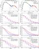 |
Fig. 3 Observed SED and radial profiles plotted along with simulated data from our one-component (left column) and two-component best-fit models (right column). In the SED plots, red data points are our new Herschel data, the light blue line represents the available Spitzer/IRS spectrum, blue points represent synthetic photometry extracted from this spectrum in order to consider them for the model fitting, gray points illustrate the photosphere subtracted photometry longward of 10 μm, and remaining points are ancillary data from the literature. Green points represent the data used for the normalization of the stellar spectrum. Data longward of 10 μm have been considered for the disk model fitting. In the radial profile plots, the thick black line represents the stellar contribution (an observation of the PSF reference star α Boo scaled to the stellar flux of HIP 17439), with its width representing the difference between major axis and minor axis. The remaining lines represent the model data and points with uncertainties represent the observed profiles. The major axis is plotted in red, the minor axis in blue. In the right column showing the results for the two-component fit, dotted lines illustrate the contribution of the two-components (inner/warm and outer/cold). |
In the previous section, we found indications that the disk is either radially very extended (from <65 au to >125 au, see values for Adisk in Table 4), or is composed of multiple belts of dust. A final conclusion was, however, not possible. To investigate the two scenarios and to further constrain the dust spatial distribution and composition, we now perform detailed analytical5 model fitting to the SED and the radial profiles of the system simultaneously.
3.1. Single-component model with variable radial width
The standard approach for modeling spatially resolved data of debris disks used in the context of Herschel/DUNES employs a disk model composed of a single disk component (Löhne et al. 2012; Ertel 2012). The one-component model we consider here is described by two power-laws. The spatial distribution of the dust is described by a power-law radial surface density distribution (exponent α) with inner radius Rin and outer radius Rout. The differential size distribution of the dust grains is described by a power-law (exponent γ) with lower grain size amin and upper grain size amax. In the present work, amax has been fixed to a reasonably large value of 2 mm, so that the effect of this parameter is negligible for reasonably steep grain size distributions (γ < −3.0). Although larger values of γ are considered in the parameter space explored, our best-fit values lie well below −3.0. Absorption coefficients of the dust grains (assumed to be spherical and compact) are computed employing Mie theory assuming the dust to be composed of astronomical silicate (Draine 2003). Composition and size distribution of the dust grains are thereby assumed to be the same throughout the whole disk. The dust mass M1mm in grains up to 1 mm (different from the value of amax because 1 mm is a common value used in the literature that permits easier comparison with other studies) and the disk inclination θ from face-on orientation completes the suit of model parameters. For the fitting we consider a total of 98 data points (SED and radial profile points as illustrated in Fig. 3).
To fit this model to the data, we use the tool SAnD described in detail by Ertel et al. (2012a) and Ertel (2012), and applied to spatially resolved data in Löhne et al. (2012) and Ertel (2012). It uses a simulated annealing approach to find the global best-fit parameters in a high dimensional parameter space. The parameter space explored in this approach is summarized in Table 5 along with the best-fit parameters found. The resulting best-fit SED and profiles are shown in the left column of Fig. 3.
Parameter space explored and best-fit values for the one-component model (top), and the two-component model (bottom).
Comparing the data observed and simulated from our one-component best-fit model, we find that most observations are well reproduced by the model. However, there is a significant deviation for the 100 μm profile along the major axis. Along this axis, the modeled profile is significantly less extended than the observed one. Nonetheless, the overall reduced χ2 is reasonably low (2.35) and considering the whole data set, this deviation may or may not be considered as critical.
A more important indication that the model used is unable to reproduce the data in a reasonable way is the set of best-fit parameters derived. These parameters indicate a very broad disk ranging from a few au up to few hundreds of au from the star with a surface density that is approximately constant. The formation of such a disk would be hard to explain. A constant surface density would be expected from a transport dominated disk (spatial distribution of the dust due to Poynting-Robertson drag dominates over local production due to collisions). Table 5 lists the collisional life time tcoll and Poynting-Robertson life time tPR for our model at the inner and outer radius of the disk. Poynting-Robertson life times are computed following Gustafson (1994) assuming grains with β = 0.5 with β being the ratio between radiation pressure force and gravitational force. Indeed, tPR and tcoll of the dust in our best-fit are of the same order, suggesting that transport mechanisms may have a significant contribution to the dust dynamics.
Estimating lifetimes for β = 0.5 grains, we implicitly assumed the grains close to the blowout size to be the most abundant in the disk. However, the grains around HIP 17439 may not reach β = 0.5, at least assuming spherical compact grains of standard composition (e.g. astronomical silicate or silicate-ice mixtures; e.g., Kirchschlager & Wolf 2013). As a result, even smaller, submicron-sized grains may be able to stay in bound orbits drifting inward to the star. Reidemeister et al. (2011) have demonstrated how disks around low-luminosity stars, where the blowout limit does not exist, may become transport-dominated even at high levels of the optical depth and thus relatively short collisional lifetimes. This may become even more efficient, if additional processes such as stellar winds are operating in the system.
However, the transport-dominated scenario faces some difficulties. One of them is that, whereas transport should be the most efficient for submicron sizes, the smallest grains found by our fitting are a few microns in size. This discrepancy can potentially be mitigated in several ways, for instance by changing assumptions about the grains properties (chemical composition, porosity, etc.). Another, more serious difficulty is that in this scenario the majority of the dust would have to be produced through collisions of larger bodies close to the outer edge of the disk, suggesting a significant amount of planetesimals at few hundreds of au from the star (~200 au or larger considering the uncertainties on Rout), which at least remains questionable. While an even smaller Rout would still be possible within the error bars, this needs to be compensated by changes in other parameters such as an outwards increasing surface density slope.
An alternative explanation to the transport dominated disk would be that the dust is produced locally throughout the whole disk with a local production rate that results in a constant surface density. To check whether this is feasible, we employ an analytic model of dust production in a steady-state collisional cascade, operating in a planetesimal disk (Löhne et al. 2008). We assume that the planetesimal disk initially had a solid surface density of the standard minimum mass solar nebula (MMSN) model (Weidenschilling 1977; Hayashi 1981), Σ = 1M⊕ au-2(r/au)− 3/2, and consider two possible mechanisms of the cascade activation. One is self-stirring, in which the cascade is assumed to start at a distance r at the moment when the 1000 km-sized planetesimals form there (Kenyon & Bromley 2008). In another case the cascade is ignited by the stirring front from a planet residing inside the disk (Mustill & Wyatt 2009). The mass of the central star is set to M⋆ = 0.7 M⊙. We assume that 10% of the available MMSN mass in solids went into formation of planetesimals up to 100 km in radius. The “primordial” slope of the differential mass distribution of planetesimals (i.e., that of the planetesimals that are sufficiently big to have collisional lifetimes longer than the time elapsed from the cascade ignition) is taken to be qp = 1.87 (cf. Löhne et al. 2008), which corresponds to a slope of the differential size distribution of γ = −3.61 assuming a constant bulk density of bodies of different size (n(a)da ∝ aγda ∝ m2 − 3qdm). For the mean eccentricities and inclinations of dust-producing planetesimals after the ignition of the cascade, we adopt e ~ 2I = 0.1. The critical shattering energy  is chosen as in Benz & Asphaug (1999). In the planetary stirring case, we assume a Jupiter-mass planet with a semi-major axis of 10 au and an orbital eccentricity of 0.1.
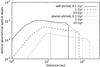 |
Fig. 4 Radial profiles of the vertical geometrical optical depth of a steady-state debris disk stirred by embedded Pluto-size objects (self-stirred, black lines) and by a planet in the inner cavity of the disk (planet-stirred, gray lines), and at different time instants: after 0.1 Gyr (solid), 1 Gyr (dashed), and 10 Gyr (dot-dashed) after the beginning of the collisional evolution. The lines of the planet-stirred case have been scaled by a factor of 1.1 for better visibility. |
Typical results for one particular set of parameters, in the form of the radial profiles of the disk’s vertical optical depth τ⊥, are presented in Fig. 4. The inner parts of the modeled disk (≲10 au) have τ⊥ increasing outward with a slope of 7/3, as expected in the case where the collisional age of the system is longer than the collisional lifetime of the largest planetesimals (see, e.g., Kennedy & Wyatt 2010; Wyatt et al. 2012). Farther out from the star, the profiles change to a nearly horizontal plateau, whose outer edge corresponds to the current position of the stirring front. Both the knee between the regions of increasing and constant τ⊥ and the outer edge of the disk moves to larger distances at later times. Thus, these simulations seem to be able to yield broad disks with a nearly constant τ⊥. However, it proves very difficult to get a disk extending to more than ~100 au, as required to reproduce the observations of the HIP 17439 disk. Varying the parameters of the model would not substantially change the results. Furthermore, as argued before against the scenario of a transport dominated disk, it is unlikely that sufficient mass in solids can be available at hundreds of au from the star. Even if it is, it would be difficult for Pluto-sized stirrers to form in the disk at those distances in ~1 Gyr. Moreover, in both planetary and self-stirring scenarios, at such large distances from the star only small bodies – which are in the strength regime and are harder to break – have collisional times shorter than the age of the system, and so only little dust is produced. This explains the second knee in Fig. 4 where τ⊥ starts to drop (at ~120 au in the 10 Gyr curves). We note, however, that the current planetesimal formation models are very uncertain, being very sensitive, for instance, to the assumed initial sizes of the seed planetesimals (Kenyon & Bromley 2010). Besides, there exist alternative mechanisms to rapidly form sufficiently large stirrers at large distances from the star, based on concentration by instabilities followed by local clumping (e.g., Johansen et al. 2012).
We summarize that we cannot rule out the broad ring model observationally due to the limited angular resolution and large uncertainties in the radial profiles. Furthermore, we cannot rule it out theoretically, since our modeling does not cover all possible scenarios, is limited by some assumptions, and not all parameters of the models have been fully explored (this is beyond the scope of this paper and we refer here to a subsequent paper by Schüppler et al., in prep.). However, based on the combination of the facts that the fit of this model to the data is imperfect and that our modeling did not result in any plausible scenario that could explain such a broad, extended disk, we conclude that such a scenario is rather unlikely.
3.2. Adding a second disk component
The results from our first fitting approach demonstrate that a single power-law disk model with the same dust composition and grain size distribution over the whole disk is unable to reproduce all data simultaneously. This is because any such disk model that results in sufficiently extended emission at 100 μm also results in significantly extended emission at 70 μm, which is not observed. Possible ways to improve over such a model would in general require an extension of it that can be considered as an additional disk component. In such a case, the outer component producing the extended emission at 100 μm must have properties that result in very low emission at 70 μm. These might be a large lower grain size resulting in a low emissivity at this wavelength and/or in a low temperature, or a large distance from the star also resulting in a low temperature (the distance from the star is, however, constrained by the extent of the disk images).
To explore these possibilities, we set up a new model featuring two independent power-law disk components each of which is identical to the single-component model used before, with slightly different sets of free and fixed parameters, as described in the following and listed in Table 5. These two components are weighted against each other and added up to the final model. Thus, for each component i (i ∈ [1,2]) there is an inner disk radius Rin,i, an outer disk radius Rout,i, an exponent αi, a lower grain size amin,i, an upper grain size amax,i, an exponent γi, and a dust mass M1mm,i in grains up to 1 mm in size. On the other hand, the inclination θ is assumed to be the same for both components. While this assumption might not be fulfilled, the 70 μm emission (most constraining the orientation of any assumed inner component) is barely resolved and thus our assumption does not significantly affect the results. Furthermore, we now consider two possible compositions of the dust – pure astronomical silicate (Draine 2003) and a 1:1 mixture of astronomical silicate and ice (Li & Greenberg 1998; Löhne et al. 2012; Ertel et al. 2012a). The volume fraction  of water ice in the silicate and ice dust grains is initially assumed to be the same for both components. In addition, we consider sublimation of the water ice in a way that the ice is replaced by vacuum if the grain temperature exceeds the sublimation temperature of the ice (Lebreton et al. 2012). Finally, we fix the outer radius of both components to 500 au. This allows us to further limit the number of free parameters to be fitted. The consequence in the model is that the surface density profile of both components is most probably forced to be decreasing outwards which results in two overlapping disk components that can be interpreted as two belts where the emission of each belt is dominated by its inner rim, respectively. The values of αi are then a measure of the width of each belt, and if the slope of the surface density of the inner belt is steep enough, the two components can be considered as detached. This way we have a total of 12 parameters to be fitted, of which M1mm,i (technically, the total mass and the mass ratio of the two components) are determined for each set of the other 10 parameters using a downhill χ2 minimization.
In order to explore a 10-dimensional parameter space, we use a hybrid approach between a precomputed model grid and the simulated annealing approach of SAnD. We use the tool GRaTer (Augereau et al. 1999; Lebreton et al. 2012; Löhne et al. 2012) to compute and store a grid of model data for each of the two components separately. On these grids of precomputed model data, we perform model fitting using a simulated annealing approach analogous to that used by SAnD. We combine for each step of the simulated annealing random walk one simulated data set from each of the two model grids and fit them to the data after proper scaling. Uncertainties on the best-fit parameters are estimated analogous to the approach used in SAND. In order to not confuse the two components in the error estimation, we ensure that Rin,1 < Rin,2 for each step.
The effectively explored parameter space, the resulting best-fit parameters, and the uncertainties on them are listed in Table 5. The SED and radial profiles simulated for this best-fit model are shown in the right panel of Fig. 3. It is important to note that given the high dimensional and extremely complex parameter space and the fact that we can only perform a limited number of runs in a reasonable time, we cannot claim anymore having found the global best-fit in the parameter space. However, we performed in total 10 independent runs with different limitations of the parameter space, all end up in the same sink of χ2 in the parameter space and do not find a deeper one.
We are able to significantly improve the fit to the 100 μm major axis profile without significantly degrading the fit to the other data. The constraints on the disk parameters are in general weak in this approach due to the intrinsic degeneracies of the model and the low spatial resolution of the data. Furthermore, models similar to our one-component best-fit model are included in the parameter space of both components. In the previous section, we already found that this model results in a fit of limited, but still acceptable quality (χ2 = 2.35). Thus, one of the two components in the present approach alone can reproduce the data sufficiently within 3σ uncertainties of the model parameters, in which case the other component can assume nearly arbitrary values. This is a major source of the large 3σ uncertainties on the model parameters. The best-fit two-component model consists of two well detached components both of which are extended disks with inner radii of ~30 au and ~90 au, respectively, and with outwards decreasing surface density profiles. Both components are collision dominated. The vertical optical depth is by a factor of ~3.5 higher for the inner component compared to the outer one. Deviations from standard parameters expected from such fits are the rather steep grain size distributions and the large lower grain size in both components, in particular in the outer component. However, the uncertainties for all these parameters are large and nearly all parameters are consistent with standard values (micron or sub-micron sized for the smallest grains, a standard value of − 3.5 for the slope of the differential size distribution) within 3σ fitting uncertainties.
The fact that the constraints on the parameters of the best-fit two-component model are weak raises the question whether a normal ring of debris at few tens of au and an additional halo of small, barely bound grains produced in this ring and drawn to large orbits by radiation pressure or stellar winds might reproduce the data as well. While the grains in such a halo should be the smallest grains present in the system, we note that our best-fit result of the two-component model suggests that the emission in the outer disk component is most likely dominated by larger grains than that of the inner component. While we cannot completely rule out that the outer disk is composed mostly of small grains due to the barely constrained outer disk parameters, we rate this scenario as very unlikely. Such small grains (a ~ 1 μm) barely emit at wavelengths as long as 100 μm, but emit more efficiently at shorter wavelength. This is inconsistent with our observation that the outer disk becomes visible only at 100 μm and longer, as long as the other model parameters do not assume very extreme values like a constant surface density, which would then be again inconsistent with a halo. Furthermore, given the luminosity of the star being at the border to not producing blow-out grains at all, it heavily depends on the parameters of the dust (e.g., composition, density, porosity, e.g., Kirchschlager & Wolf 2013) whether there are barely bound grains at all.
4. Conclusions
We have spatially resolved for the first time the debris disk around HIP 17439. The disk morphology changes significantly from 70 μm to 100 μm suggesting a very extended disk or a disk composed of multiple components to be present. Our simultaneous multi-wavelength modeling of all available data of this disk including the radial profiles obtained from our resolved observations shows that a single-component model does reproduce most of the data in a reasonable way but fails in reproducing the profiles at 70 μm and 100 μm simultaneously, i.e., in reproducing the change in disk morphology between these two wavelengths. We furthermore have demonstrated with an analytical approach that the resulting best-fit model as well as most models allowed within 3σ of the uncertainties on the model parameters are physically unlikely. In contrast, we have demonstrated that a two-component disk model is able to reproduce all data simultaneously and results in a physically more plausible result. This best-fit model is composed of two rings of debris located at ~30 au and at ~90 au from the star. The dust mass derived from our model puts the disk among the least massive debris disks spatially resolved so far. Depending on the disk geometry (which strongly affects the vertical optical depth, but could not be unambiguously constrained in the present work), transport mechanisms may play a significant role in the dust dynamics. This potentially makes the disk similar to that of HD 207129 (Löhne et al. 2012), and interesting to study dust dynamics and evolution in debris disks with low surface density. It is also particularly interesting as the disk does not have a particularly low fractional luminosity compared to other debris disks detected by Spitzer or Herschel (e.g., Bryden et al. 2006; Beichman et al. 2006; Hillenbrand et al. 2008; Bryden et al. 2009; Eiroa et al. 2013). This means that in a significant fraction of known debris disks transport mechanisms might not be negligible. This is in contrast to the estimates by Wyatt (2005), who assumed debris disks to be narrow rings which might not be the case for HIP 17439.
In the lack of higher spatial resolution, which would require a higher sensitivity to surface brightness than can be achieved with current instruments (including ALMA judged from our best-fit models, see predictions by Ertel et al. 2012b, their Fig. 5, left) only spatially resolved multi-wavelength observations and the detailed simultaneous modeling of all available data were able to reveal the multi-component (or possible extremely extended) structure of the disk. A more detailed modeling of the system’s dust distribution considering self consistently the dynamical and collisional evolution of both the planetesimals and the dust in order to investigate whether the scenarios found are physically really plausible is beyond the scope of this paper. We postpone this to a later study (Schüppler et al., in prep.). This study will potentially reveal the conditions under which the scenarios found are physical and further constrain possible disk architectures, including the locations of dust-producing planetesimal belts analogous to previous studies for other objects (Reidemeister et al. 2011; Löhne et al. 2012).
In recent years, more an increasing number of debris disks have been modeled in detail and revealed to consist of several components, more or less similar to the architecture of our own solar system (e.g., ϵ Eri: Backman et al. 2009; HR 8799: Su et al. 2009; η Crv: Matthews et al. 2010; HD 107146: Ertel et al. 2011; Fomalhaut: Acke et al. 2012, Su et al. 2013; HD 32297: Donaldson et al. 2013; Vega: Su et al. 2013; γ Dor: Broekhoven-Fiene et al. 2013; κ CrB: Bonsor et al. 2013, including exozodiacal dust systems, e.g., around Vega: Absil et al. 2006, Defrère et al. 2011; Fomalhaut: Absil et al. 2009, Mennesson et al. 2013, Lebreton et al. 2013; β Pic: Defrère et al. 2012). Some of these stars harbor (candidate) planetary companions at a similar distance from the star as the dust (i.e., HR8799: Marois et al. 2008, Martínez-Arnáiz et al. 2010; Fomalhaut: Kalas et al. 2008; β Pic: Lagrange et al. 2010; our solar system), possibly being responsible for the gap between the multiple components of the disk. This raises the question of whether such a companion might also exist around HIP 17439. It is interesting to note that the configuration of the two rings as found by the present study closely resembles structures simulated by Ertel et al. (2012b, their model sequence III), suggesting that a single, Jovian mass planet might be sufficient to explain the configuration of the belts in our best-fit model. However, it is important not to over interpret these similarities. On the one hand, the parameters found from our best-fit come with large uncertainties. On the other hand, it was not the goal of Ertel et al. (2012b) to produce highly accurate structures suited for comparison with real observations, but to produce reasonable structures to be used for the subsequent analysis of their observability carried out. More detailed conclusions require better constraints on the configuration of the system as well as dedicated simulations of planet-disk interaction. A clear proof that planets are responsible for the multi-component structures in these systems would allow to study a new class of planets (large separation form the host star, possible low/intermediate mass or higher age compared to the planets discovered at such distance by direct imaging or hinted at by long term radial velocity trends) not accessible to any other observing technique available.
The Cornell Atlas of Spitzer/IRS Sources (CASSIS) is a product of the Infrared Science Center at Cornell University, supported by NASA and JPL.
See PICC-ME-TN-036, Sect. 1 for details.
See SPIRE observer’s manual, Sect. 3.2.2 for details.
SPIRE observer’s manual, Sect. 5.2.
Here, the term “analytical” refers to fitting of the observational data to spatial and size distributions of dust, assumed to be power laws. It is used to distinguish this kind of modeling from collisional and dynamical simulations that address physical processes of the dust production and evolution and deal with dust distributions that are more complex than power laws.
Acknowledgments
S. Ertel and J.-C. Augereau thank the French National Research Agency (ANR, contract ANR-2010 BLAN-0505-01, EXOZODI) and PNP-CNES for financial support. C. Eiroa, J. Maldonado, J. P. Marshall, and B. Montesinos are partially supported by Spanish grant AYA 2011-26202. A. V. Krivov acknowledges support from the DFG, grant Kr 2164/10-1. T. Löhne acknowledges support from the DFG, grant Lo 1715/1-1. R. Liseau acknowledges the continued support by the Swedish National Space Board (SNSB). We thank the anonymous referee for valuable comments. S. Ertel thanks K. Ertel for general support.
References
- Absil, O., di Folco, E., Mérand, A., et al. 2006, A&A, 452, 237 [NASA ADS] [CrossRef] [EDP Sciences] [Google Scholar]
- Absil, O., Mennesson, B., Le Bouquin, J., et al. 2009, ApJ, 704, 150 [NASA ADS] [CrossRef] [Google Scholar]
- Acke, B., Min, M., Dominik, C., et al. 2012, A&A, 540, A125 [NASA ADS] [CrossRef] [EDP Sciences] [Google Scholar]
- Augereau, J. C., Lagrange, A. M., Mouillet, D., Papaloizou, J. C. B., & Grorod, P. A. 1999, A&A, 348, 557 [NASA ADS] [Google Scholar]
- Backman, D. E., & Paresce, F. 1993, in Protostars and Planets III, eds. E. H. Levy, & J. I. Lunine, 1253 [Google Scholar]
- Backman, D., Marengo, M., Stapelfeldt, K., et al. 2009, ApJ, 690, 1522 [NASA ADS] [CrossRef] [Google Scholar]
- Beichman, C. A., Bryden, G., Rieke, G. H., et al. 2005, ApJ, 622, 1160 [NASA ADS] [CrossRef] [Google Scholar]
- Beichman, C. A., Bryden, G., Stapelfeldt, K. R., et al. 2006, ApJ, 652, 1674 [NASA ADS] [CrossRef] [Google Scholar]
- Benz, W., & Asphaug, E. 1999, Icarus, 142, 5 [NASA ADS] [CrossRef] [Google Scholar]
- Bertone, E., Buzzoni, A., Chávez, M., & Rodríguez-Merino, L. H. 2004, AJ, 128, 829 [NASA ADS] [CrossRef] [Google Scholar]
- Bonsor, A., Kennedy, G. M., Crepp, J. R., et al. 2013, MNRAS, 431, 3025 [NASA ADS] [CrossRef] [Google Scholar]
- Broekhoven-Fiene, H., Matthews, B. C., Kennedy, G. M., et al. 2013, ApJ, 762, 52 [NASA ADS] [CrossRef] [Google Scholar]
- Brott, I., & Hauschildt, P. H. 2005, in The Three-Dimensional Universe with Gaia, eds. C. Turon, K. S. O’Flaherty, & M. A. C. Perryman, ESA SP, 576, 565 [Google Scholar]
- Bryden, G., Beichman, C. A., Trilling, D. E., et al. 2006, ApJ, 636, 1098 [NASA ADS] [CrossRef] [Google Scholar]
- Bryden, G., Beichman, C. A., Carpenter, J. M., et al. 2009, ApJ, 705, 1226 [NASA ADS] [CrossRef] [Google Scholar]
- Chen, C. H., Sargent, B. A., Bohac, C., et al. 2006, ApJS, 166, 351 [NASA ADS] [CrossRef] [Google Scholar]
- Chen, C. H., Li, A., Bohac, C., et al. 2007, ApJ, 666, 466 [NASA ADS] [CrossRef] [Google Scholar]
- Cutri, R. M., & et al. 2012, VizieR Online Data Catalog, II/307 [Google Scholar]
- Defrère, D., Absil, O., Augereau, J.-C., et al. 2011, A&A, 534, A5 [NASA ADS] [CrossRef] [EDP Sciences] [Google Scholar]
- Defrère, D., Lebreton, J., Le Bouquin, J.-B., et al. 2012, A&A, 546, L9 [NASA ADS] [CrossRef] [EDP Sciences] [Google Scholar]
- Dominik, C., & Decin, G. 2003, ApJ, 598, 626 [NASA ADS] [CrossRef] [Google Scholar]
- Donaldson, J. K., Lebreton, J., Roberge, A., Augereau, J.-C., & Krivov, A. V. 2013, ApJ, 772, 17 [NASA ADS] [CrossRef] [Google Scholar]
- Draine, B. T. 2003, ApJ, 598, 1017 [NASA ADS] [CrossRef] [Google Scholar]
- Eiroa, C., Fedele, D., Maldonado, J., et al. 2010, A&A, 518, L131 [NASA ADS] [CrossRef] [EDP Sciences] [Google Scholar]
- Eiroa, C., Marshall, J. P., Mora, A., et al. 2013, A&A, 555, A11 [NASA ADS] [CrossRef] [EDP Sciences] [Google Scholar]
- Engelbracht, C. W., Blaylock, M., Su, K. Y. L., et al. 2007, PASP, 119, 994 [NASA ADS] [CrossRef] [Google Scholar]
- Ertel, S. 2012, Ph.D. Thesis, Christian-Albrechts-Universität zu Kiel, http://eldiss.uni-kiel.de/macau/receive/dissertation_diss_00007810 [Google Scholar]
- Ertel, S., Wolf, S., Metchev, S., et al. 2011, A&A, 533, A132 [NASA ADS] [CrossRef] [EDP Sciences] [Google Scholar]
- Ertel, S., Wolf, S., Marshall, J. P., et al. 2012a, A&A, 541, A148 [NASA ADS] [CrossRef] [EDP Sciences] [Google Scholar]
- Ertel, S., Wolf, S., & Rodmann, J. 2012b, A&A, 544, A61 [NASA ADS] [CrossRef] [EDP Sciences] [Google Scholar]
- Fernandes, J. M., Vaz, A. I. F., & Vicente, L. N. 2011, A&A, 532, A20 [NASA ADS] [CrossRef] [EDP Sciences] [Google Scholar]
- Flower, P. J. 1996, ApJ, 469, 355 [NASA ADS] [CrossRef] [Google Scholar]
- Garcés, A., Ribas, I., & Catalán, S. 2010, in Pathways Towards Habitable Planets, eds. V. Coudé Du Foresto, D. M. Gelino, & I. Ribas, ASP Conf. Ser., 430, 437 [Google Scholar]
- Gordon, K. D., Rieke, G. H., Engelbracht, C. W., et al. 2005, PASP, 117, 503 [NASA ADS] [CrossRef] [Google Scholar]
- Gordon, K. D., Engelbracht, C. W., Fadda, D., et al. 2007, PASP, 119, 1019 [NASA ADS] [CrossRef] [Google Scholar]
- Gray, R. O., Corbally, C. J., Garrison, R. F., et al. 2006, AJ, 132, 161 [NASA ADS] [CrossRef] [Google Scholar]
- Griffin, M. J., Abergel, A., Abreu, A., et al. 2010, A&A, 518, L3 [Google Scholar]
- Gustafson, B. A. S. 1994, Ann. Rev. Earth Planet. Sci., 22, 553 [Google Scholar]
- Hauck, B., & Mermilliod, M. 1998, A&AS, 129, 431 [NASA ADS] [CrossRef] [EDP Sciences] [Google Scholar]
- Hayashi, C. 1981, Prog. Theor. Phys. Suppl., 70, 35 [NASA ADS] [CrossRef] [MathSciNet] [Google Scholar]
- Hillenbrand, L. A., Carpenter, J. M., Kim, J. S., et al. 2008, ApJ, 677, 630 [Google Scholar]
- Holmberg, J., Nordström, B., & Andersen, J. 2009, A&A, 501, 941 [NASA ADS] [CrossRef] [EDP Sciences] [Google Scholar]
- Houck, J. R., Roellig, T. L., van Cleve, J., et al. 2004, ApJS, 154, 18 [NASA ADS] [CrossRef] [Google Scholar]
- Ishihara, D., Onaka, T., Kataza, H., et al. 2010, VizieR Online Data Catalog: II/297 [Google Scholar]
- Johansen, A., Youdin, A. N., & Lithwick, Y. 2012, A&A, 537, A125 [NASA ADS] [CrossRef] [EDP Sciences] [Google Scholar]
- Kalas, P., Graham, J. R., Chiang, E., et al. 2008, Science, 322, 1345 [NASA ADS] [CrossRef] [PubMed] [Google Scholar]
- Kennedy, G. M., & Wyatt, M. C. 2010, MNRAS, 405, 1253 [NASA ADS] [Google Scholar]
- Kennedy, G. M., Wyatt, M. C., Sibthorpe, B., et al. 2012, MNRAS, 426, 2115 [NASA ADS] [CrossRef] [Google Scholar]
- Kenyon, S. J., & Bromley, B. C. 2004, AJ, 127, 513 [NASA ADS] [CrossRef] [Google Scholar]
- Kenyon, S. J., & Bromley, B. C. 2008, ApJS, 179, 451 [NASA ADS] [CrossRef] [Google Scholar]
- Kenyon, S. J., & Bromley, B. C. 2010, ApJS, 188, 242 [NASA ADS] [CrossRef] [Google Scholar]
- Kirchschlager, F., & Wolf, S. 2013, A&A, 552, A54 [NASA ADS] [CrossRef] [EDP Sciences] [Google Scholar]
- Koerner, D. W., Kim, S., Trilling, D. E., et al. 2010, ApJ, 710, L26 [NASA ADS] [CrossRef] [Google Scholar]
- Krivov, A. V. 2010, RA&A, 10, 383 [Google Scholar]
- Lagrange, A.-M., Bonnefoy, M., Chauvin, G., et al. 2010, Science, 329, 57 [NASA ADS] [CrossRef] [PubMed] [Google Scholar]
- Lebouteiller, V., Barry, D. J., Spoon, H. W. W., et al. 2011, ApJS, 196, 8 [NASA ADS] [CrossRef] [Google Scholar]
- Lebreton, J., Augereau, J.-C., Thi, W.-F., et al. 2012, A&A, 539, A17 [NASA ADS] [CrossRef] [EDP Sciences] [Google Scholar]
- Lebreton, J., van Lieshout, R., Augereau, J.-C., et al. 2013, A&A, 555, A146 [NASA ADS] [CrossRef] [EDP Sciences] [Google Scholar]
- Li, A., & Greenberg, J. M. 1998, A&A, 331, 291 [NASA ADS] [Google Scholar]
- Löhne, T., Krivov, A. V., & Rodmann, J. 2008, ApJ, 673, 1123 [NASA ADS] [CrossRef] [Google Scholar]
- Löhne, T., Augereau, J.-C., Ertel, S., et al. 2012, A&A, 537, A110 [NASA ADS] [CrossRef] [EDP Sciences] [Google Scholar]
- Maldonado, J., Martínez-Arnáiz, R. M., Eiroa, C., Montes, D., & Montesinos, B. 2010, A&A, 521, A12 [NASA ADS] [CrossRef] [EDP Sciences] [Google Scholar]
- Mamajek, E. E., & Hillenbrand, L. A. 2008, ApJ, 687, 1264 [NASA ADS] [CrossRef] [Google Scholar]
- Marois, C., Macintosh, B., Barman, T., et al. 2008, Science, 322, 1348 [NASA ADS] [CrossRef] [PubMed] [Google Scholar]
- Martínez-Arnáiz, R., Maldonado, J., Montes, D., Eiroa, C., & Montesinos, B. 2010, A&A, 520, A79 [NASA ADS] [CrossRef] [EDP Sciences] [Google Scholar]
- Matthews, B. C., Sibthorpe, B., Kennedy, G., et al. 2010, A&A, 518, L135 [NASA ADS] [CrossRef] [EDP Sciences] [Google Scholar]
- Mennesson, B., Absil, O., Lebreton, J., et al. 2013, ApJ, 763, 119 [NASA ADS] [CrossRef] [Google Scholar]
- Moór, A., Ábrahám, P., Derekas, A., et al. 2006, ApJ, 644, 525 [NASA ADS] [CrossRef] [Google Scholar]
- Moshir, M., et al. 1990, in IRAS Faint Source Catalogue, version 2.0 [Google Scholar]
- Mustill, A. J., & Wyatt, M. C. 2009, MNRAS, 399, 1403 [NASA ADS] [CrossRef] [Google Scholar]
- Ott, S. 2010, in Astronomical Data Analysis Software and Systems XIX, eds. Y. Mizumoto, K.-I. Morita, & M. Ohishi, ASP Conf. Ser., 434, 139 [Google Scholar]
- Perryman, M. A. C., Lindegren, L., Kovalevsky, J., et al. 1997, A&A, 323, L49 [NASA ADS] [Google Scholar]
- Pilbratt, G. L., Riedinger, J. R., Passvogel, T., et al. 2010, A&A, 518, L1 [CrossRef] [EDP Sciences] [Google Scholar]
- Poglitsch, A., Waelkens, C., Geis, N., et al. 2010, A&A, 518, L2 [NASA ADS] [CrossRef] [EDP Sciences] [Google Scholar]
- Reidemeister, M., Krivov, A. V., Stark, C. C., et al. 2011, A&A, 527, A57 [NASA ADS] [CrossRef] [EDP Sciences] [Google Scholar]
- Santos, N. C., Israelian, G., & Mayor, M. 2004, A&A, 415, 1153 [NASA ADS] [CrossRef] [EDP Sciences] [Google Scholar]
- Silverstone, M. D. 2000, Ph.D. Thesis, University of California, Los Angeles [Google Scholar]
- Skrutskie, M. F., Cutri, R. M., Stiening, R., et al. 2006, AJ, 131, 1163 [NASA ADS] [CrossRef] [Google Scholar]
- Su, K. Y. L., Rieke, G. H., Stapelfeldt, K. R., et al. 2009, ApJ, 705, 314 [NASA ADS] [CrossRef] [Google Scholar]
- Su, K. Y. L., Rieke, G. H., Malhotra, R., et al. 2013, ApJ, 763, 118 [NASA ADS] [CrossRef] [Google Scholar]
- Swinyard, B. M., Ade, P., Baluteau, J.-P., et al. 2010, A&A, 518, L4 [Google Scholar]
- Torres, C. A. O., Quast, G. R., da Silva, L., et al. 2006, A&A, 460, 695 [NASA ADS] [CrossRef] [EDP Sciences] [Google Scholar]
- Valenti, J. A., & Fischer, D. A. 2005, VizieR Online Data Catalog, 215, 90141 [NASA ADS] [Google Scholar]
- van Leeuwen, F. 2007, A&A, 474, 653 [NASA ADS] [CrossRef] [EDP Sciences] [Google Scholar]
- Weidenschilling, S. J. 1977, Ap&SS, 51, 153 [Google Scholar]
- Werner, M. W., Roellig, T. L., Low, F. J., et al. 2004, ApJS, 154, 1 [Google Scholar]
- Wyatt, M. C. 2005, A&A, 433, 1007 [NASA ADS] [CrossRef] [EDP Sciences] [Google Scholar]
- Wyatt, M. C. 2008, ARA&A, 46, 339 [NASA ADS] [CrossRef] [Google Scholar]
- Wyatt, M. C., Kennedy, G., Sibthorpe, B., et al. 2012, MNRAS, 424, 1206 [NASA ADS] [CrossRef] [Google Scholar]
All Tables
Parameter space explored and best-fit values for the one-component model (top), and the two-component model (bottom).
All Figures
|
Fig. 1 Herschel/PACS and Herschel/SPIRE observations of HIP 17439. The band is noted in the upper left corner of each panel. The white circle in the lower left of each panel illustrates the FWHM of the theoretical, circular PSF. |
| In the text | |
|
Fig. 2 Original images and deconvolved images at the three Herschel/PACS bands. Image type, wavelength and deconvolution method are noted in the upper left corner of each panel, respectively. The images are oriented north up, east left. Contours denote positive surface brightness values and are drawn in steps of 10% of the peak surface brightness. The color scale is linear and ranges from zero to the peak surface brightness. |
| In the text | |
|
Fig. 3 Observed SED and radial profiles plotted along with simulated data from our one-component (left column) and two-component best-fit models (right column). In the SED plots, red data points are our new Herschel data, the light blue line represents the available Spitzer/IRS spectrum, blue points represent synthetic photometry extracted from this spectrum in order to consider them for the model fitting, gray points illustrate the photosphere subtracted photometry longward of 10 μm, and remaining points are ancillary data from the literature. Green points represent the data used for the normalization of the stellar spectrum. Data longward of 10 μm have been considered for the disk model fitting. In the radial profile plots, the thick black line represents the stellar contribution (an observation of the PSF reference star α Boo scaled to the stellar flux of HIP 17439), with its width representing the difference between major axis and minor axis. The remaining lines represent the model data and points with uncertainties represent the observed profiles. The major axis is plotted in red, the minor axis in blue. In the right column showing the results for the two-component fit, dotted lines illustrate the contribution of the two-components (inner/warm and outer/cold). |
| In the text | |
|
Fig. 4 Radial profiles of the vertical geometrical optical depth of a steady-state debris disk stirred by embedded Pluto-size objects (self-stirred, black lines) and by a planet in the inner cavity of the disk (planet-stirred, gray lines), and at different time instants: after 0.1 Gyr (solid), 1 Gyr (dashed), and 10 Gyr (dot-dashed) after the beginning of the collisional evolution. The lines of the planet-stirred case have been scaled by a factor of 1.1 for better visibility. |
| In the text | |
Current usage metrics show cumulative count of Article Views (full-text article views including HTML views, PDF and ePub downloads, according to the available data) and Abstracts Views on Vision4Press platform.
Data correspond to usage on the plateform after 2015. The current usage metrics is available 48-96 hours after online publication and is updated daily on week days.
Initial download of the metrics may take a while.