| Issue |
A&A
Volume 560, December 2013
|
|
|---|---|---|
| Article Number | A81 | |
| Number of page(s) | 12 | |
| Section | Extragalactic astronomy | |
| DOI | https://doi.org/10.1051/0004-6361/201322842 | |
| Published online | 09 December 2013 | |
An optical spectroscopic survey of the 3CR sample of radio galaxies with z < 0.3
V. Implications for the unified model for FR IIs⋆
1 SISSA-ISAS, via Bonomea 265, 34136 Trieste, Italy
e-mail: This email address is being protected from spambots. You need JavaScript enabled to view it.
2 INAF − Osservatorio Astrofisico di Torino, Strada Osservatorio 20, 10025 Pino Torinese, Italy
3 INAF − Osservatorio Astronomico di Padova, Vicolo dell’Osservatorio 5, 35122 Padova, Italy
4 Space Telescope Science Institute, 3700 San Martin Drive, Baltimore, MD 21218, USA
5 INAF − Istituto di Radio Astronomia, via P. Gobetti 101, 40129 Bologna, Italy
6 Center for Astrophysical Sciences, Johns Hopkins University, 3400 N. Charles Street Baltimore, MD 21218, USA
7 INAF − Osservatorio Astronomico di Brera, via E. Bianchi 46, 23807 Merate, Italy
8 INFN − Sezione di Trieste, via Valerio 2, 34127 Trieste, Italy
Received: 14 October 2013
Accepted: 30 October 2013
Abstract
We explore the implications of our optical spectroscopic survey of 3CR radio sources with z < 0.3 for the unified model (UM) for radio-loud AGN, focusing on objects with a “edge-brightened” (FR II) radio morphology. The sample contains 33 high ionization galaxies (HIGs) and 18 broad line objects (BLOs). According to the UM, HIGs, the narrow line sources, are the nuclearly obscured counterparts of BLOs. The fraction of HIGs indicates a covering factor of the circumnuclear matter of 65% that corresponds, adopting a torus geometry, to an opening angle of 50° ± 5. No dependence on redshift and luminosity on the torus opening angle emerges. We also consider the implications for a “clumpy” torus. The distributions of total radio luminosity of HIGs and BLOs are not statistically distinguishable, as expected from the UM. Conversely, BLOs have a radio core dominance, R, more than ten times larger with respect to HIGs, as expected in case of Doppler boosting when the jets in BLOs are preferentially oriented closer to the line of sight than in HIGs. Modeling the R distributions leads to an estimate of the jet bulk Lorentz factor of Γ ~ 3−5. The test of the UM based on the radio source size is not conclusive due to the limited number of objects and because the size distribution is dominated by the intrinsic scatter rather than by projection effects. The [O II] line luminosities in HIGs and BLOs are similar but the [O III] and [O I] lines are higher in BLOs by a factor of ~2. We ascribe this effect to the presence of a line emitting region located within the walls of the obscuring torus, visible in BLOs but obscured in HIGs, with a density higher than the [O II] critical density. We find evidence that BLOs have broader [O I] and [O III] lines than HIGs of similar [O II] width, as expected in the presence of high density gas in the proximity of the central black hole. In conclusion, the radio and narrow line region (NLR) properties of HIGs and BLOs are consistent with the UM predictions when the partial obscuration of the NLR is taken into account. We also explored the radio properties of 21 3CR low ionization galaxies with a FR II radio morphology at z < 0.3. We find evidence that they cannot be part of the model that unifies HIGs and BLOs, but they are instead intrinsically different source, still reproduced by a randomly oriented population.
Key words: galaxies: active / galaxies: jets / galaxies: nuclei
Table 1 is available in electronic form at http://www.aanda.org
© ESO, 2013
1. Introduction
The unified model (UM) for active galactic nuclei (AGN) postulates that different classes of objects might actually be intrinsically identical and differ solely for their orientation with respect to our line of sight (see, e.g., Antonucci 1993 for a review). The origin of the aspect dependent classification is due to the presence of: i) circumnuclear absorbing material (usually referred to as the obscuring torus) that produces selective absorption when the source is observed at a large angle from its radio axis; ii) Doppler boosting associated with relativistic motions in AGN jets.
According to this model, for radio-loud AGN a source appears as a quasar only when its radio axis is oriented within a small cone opening around the observers line of sight (Barthel 1989). In the unification scheme of radio loud AGN (e.g., Urry & Padovani 1995) narrow-lined radio galaxies of FR II type (Fanaroff & Riley 1974) and broad-lined FR IIs together with RL QSOs, also called broad line objects (BLO), are considered to be intrinsically indistinguishable. Their different aspect (in particular the absence of broad emission lines in FR IIs) is only related to their orientation in the sky with respect to our line of sight. Therefore, the UM, in its stricter interpretation of a pure orientation scheme, predicts that narrow-line and broad-line FR II are drawn from the same parent population. Among the several pieces of evidence in favor of the UM, probably the most convincing one is the detection of broad lines in the polarized spectra of narrow-line objects (Antonucci 1982, 1984) interpreted as the result of scattered light from an otherwise obscured nucleus.
The FR II radio galaxies population consists of two main families, based on the optical narrow emission-line ratios: high ionization galaxies (HIG) and low ionization galaxies1 (LIG; Hine & Longair 1979; Jackson & Rawlings 1997; Buttiglione et al. 2010). Such a dichotomy also corresponds to a separation in nuclear properties at different wavelengths (e.g., Chiaberge et al. 2002; Hardcastle et al. 2006; Baldi et al. 2010).
In Buttiglione et al. (2010) we noted that all BLOs have a high ionization spectrum, based on the ratios between narrow emission lines. Since this spectroscopic classification should not depend on orientation (an issue that, however, we will discuss later in more detail) this suggests to consider the narrow-lined HIGs as the nuclearly obscured counterpart of the BLO population. On the other hand, LIGs appear to be a different class of AGN. In fact Laing et al. (1994) have pointed out that LIGs are unlikely to appear as quasars when seen face-on and that these should be excluded from a sample while testing the unified scheme model (see also Wall & Jackson 1997 and Jackson & Wall 1999). Therefore, in order to test the validity of the UM for RL AGN, it is necessary to treat separately FR II HIGs (with BLOs) and LIGs because of their different nuclear properties and spectroscopic classifications.
The Revised Third Cambridge Catalog 3CR (Bennett 1962a,b; Spinrad et al. 1985) is perfectly suited to test the validity and to explore the implications for the UM for local powerful radio-loud AGN. This is because it is based on the low frequency radio emission which should make it free from orientation biases. Furthermore, the results of a complete optical spectroscopic survey obtained for the 3CR radio sources, limited to z < 0.3 (Buttiglione et al. 2009, 2010, 2011) gives a robust spectral classification of all objects.
The completeness and the homogeneity of the sample, reached with the 3CR spectroscopic survey, are fundamental for obtaining results with a high statistical foundation. Thanks to these conditions, our intention is to test various predictions and to discuss the implications of the UM on the properties of the sample of 3CR FR II radio galaxies with results more robust than in previous works.
The UM validity, that can be tested with the available data, is represented by the consistency of the isotropic properties of the two sub-samples of HIGs and BLOs. According to the “zeroth-order approximation” of the AGN UM, the extended radio emission and the narrow line region (NLR) are supposed to be insensitive to orientation. The extended radio emission is the main characteristic of radio-loud AGN: it is isotropic, it extends far beyond the host galaxy dimensions, and it is not affected by absorption. The narrow lines are observed in all AGNs (except in BL Lac objects, where the beamed nuclear emission dominates the spectrum, diluting their intrinsically weak emission lines, Capetti et al. 2010) and their extent, up to kpc scales, is certainly larger than the size of the torus and they cannot be completely obscured. Thus these quantities can be compared in BLOs and HIGs to test the UM. Another important aspect of orientation is an apparent change of the radio core luminosity: since the core emission is subject to relativistic beaming effects, when the jet is pointing in a direction close to our line of sight (face-on AGN) its emission will be enhanced while, in the case the AGN is edge-on the core emission, should be de-beamed. The separation in radio core power between HIGs and BLOs can be modeled to extract information on the jet properties. In addition, the orientation scheme has also the geometric effect of producing the projected sizes of BLOs in radio images smaller than those of HIGs. Such a difference can be also used to test the validity of the UM for RL AGN.
Finally, we consider the FR II LIG sub-sample to study how they fit into in the oriented-based unified scheme, bearing in mind that Laing et al. (1994) already suggest that LIGs appear to be a intrinsically different RL AGN population from HIGs and BLOs.
The structure of this paper is as follows: in Sect. 2 we define the sample considered and list the main properties of the sources; the separation between BLOs and HIGs is critically reviewed in Sect. 3. In Sect. 4 we derive the geometric properties of the obscuring material. The implications of the UM on the radio and emission line properties are presented in Sect. 5 through 7. The role of LIGs in the UM is addressed in Sect. 8. The results are discussed in Sect. 9 and summarized in Sect. 10, where we also draw our conclusions.
2. The sample
We consider all the 3CR FR II radio sources with a limiting redshift of z < 0.3 and an optical spectrum characterized by emission lines of high ionization. As explained in the Introduction, HIGs and BLOs differ by definition for the presence of broad emission lines in their optical spectra. Finally, we also consider separately the 3CR FR II LIG sources, again with z < 0.3.
The main data for these sources are reported in Table 1. The spectroscopic data are taken from Buttiglione et al. (2009, 2011), while the spectral classification is from Buttiglione et al. (2010, 2011). The total radio luminosities at 178 MHz are from Spinrad et al. (1985), while the radio core power at 5 GHz are from the compilation of literature data presented by Baldi et al. (2010).
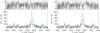 |
Fig. 1 Left panel: fit to the spectrum of 3C 133 obtained by forcing the presence of a broad Hα. Right panel: result of the fit with only narrow line components. The original spectrum is in black, the narrow lines are in green, and the broad Hα is in blue. The residuals are shown in the top panel of both figures. |
3. Are the broad lines really missing in the HIGs spectra?
BLOs are defined as the objects in which emission from a BLR is clearly detected in the optical spectra in the form of a broad Balmer line emission underlying the forbidden narrow emission lines; a fit including only narrow components leaves strong positive residuals. Conversely, a BLR is apparently missing in HIGs. But is it possible that lines are not detected in HIGs broad only because of observational limitations, such as they are hidden by the continuum emission or by the narrow emission lines, and/or they are not visible just due an insufficient quality of the spectra? In other words, how reliable is the separation between BLOs and HIGs?
In order to answer this question we looked more closely for broad lines footprints in HIGs. We focused on the Hα emission line because it is the brightest permitted emission lines in the optical spectra. We used the specfit package from the IRAF data reduction software forcing the program to fit a broad line underlying the complex of [N II]+Hα emission lines even in absence of clear residuals. We tested different line widths, fixing its value in specfit within the range 4000−8000 km s-1 as measured in BLOs. We then assessed the reliability of the presence of the broad Hα line with a likelihood ratio test (F-test, Bevington & Robinson 2003). This compares the residuals of the fit with and without an additional component in the model, taking into account the increased number of degrees of freedom. By setting a significance threshold at 95% a broad line is not detected in any HIGs with the exception of 3C 234. We then set as upper limit to the broad Hα flux 3 times the measurement errors. As an example we report in Fig. 1 the case of 3C 133, the object with the largest allowed broad line flux.
The result of this analysis is shown in Fig. 2. Buttiglione et al. (2010) noted that for BLOs there is a proportionality between the broad and narrow emission line fluxes, as a consequence of the fact that both originate from the same ionizing radiation. The average relation between the [O III] and Hα broad line fluxes derived from the BLOs is reported as the solid line in the Fig. 2. Conversely, HIGs are all (but one) located well below (by a factor of 10−1000) the relation defined by BLOs. The only object consistent with the broad Hα − [O III] ratio of BLOs is 3C 284, whose spectrum is of rather poor quality and has the lowest value of [O III] flux. We conclude that the broad Hα line flux in HIGs is significantly lower than it would have been expected based on their [O III] flux. This implies that any broad line in HIGs does not obey to the same scaling of BLOs and that the separation between the two classes is robust and reliable.
The only exception to this scheme is 3C 234 where a BLR is seen, although ~20 times fainter that one would predict from its [O III] flux. However, spectro-polarimetric studies of this source revealed that its broad lines are highly polarized and they are the ascribed to of scattered nuclear light (Antonucci 1984). This is actually one of the observational results at the very foundation of the UM. In 3C 234 we do not have a direct view of the BLR, but given its high flux, the small scattered fraction is sufficient to see a broad line in its total intensity spectrum.
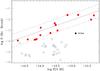 |
Fig. 2 Comparison between the narrow [O III] line and the broad Hα fluxes. Red squares are BLOs, black circles are HIGs, with empty symbols representing upper limits. The fluxes are in erg cm-2 s-1. The solid line marks the average ratio between the two emission lines as measured in BLOs, (FHα broad/F[O III] ~ 8). The dashed lines illustrate a change of a factor of 4 in this value. |
4. Geometry of the obscuring torus
Considering that our sample is complete for redshift z < 0.3 and not subject to selection biases, we can use the ratio between the number of BLOs and HIGs to study the geometry of the circumnuclear obscuring material. This analysis implicitly assumes the validity of the UM, i.e., that the differences between HIGs and BLOs are solely due to a different orientation with respect to the line of sight and to the presence of selective obscuration. We initially limit ourselves to a simple structure, assuming that it produces complete obscuration toward the nucleus when its axis forms with the line of sight an angle larger than a critical value (θc), while it leaves a free view for smaller angles, i.e., that it takes the form of a torus with sharp boundaries.
For angles smaller than θc we then expect to look inside the torus, to see the BLR and thence to observe a BLO; for angles larger than θc the BLR is obscured by the torus, thus we observe a HIG. For a randomly oriented set of sources, the probability of finding an object within the cone with an opening angle θc is P(θ < θc) = 1 − cos θc (Barthel 1989). In the complete 3CR sample for z < 0.3 we have 18 BLOs and 33 HIGs from the optical spectroscopic classification. The resulting value for the critical angle is θc = 49.7°.
In order to estimate the uncertainty on θc related to the limited size of our sample, we ran a set of Monte Carlo simulations. More specifically, we measured the distribution of the number ratio between HIGs and BLOs in 1000 realizations of a sample of 51 randomly oriented sources and derived the corresponding value of θc. This procedure yields a dispersion of 5°. The final result is then θc = 50° ± 5°.
We also split the radio sources in two sub-samples depending on the redshift. Since we are considering a flux limited sample this generally corresponds into splitting the sample at different levels of luminosity. This is aimed at verifying whether θc is constant with luminosity or, conversely, it changes for sources at higher redshift/luminosity. We have chosen a threshold that divides almost equally the objects of the sample, i.e., z = 0.15. The median luminosities of the sources in the two redshift bins differ by almost an order of magnitude, being log L178 MHz = 33.5 erg s-1 Hz-1 and log L178 MHz = 34.4 erg s-1 Hz-1 for z < 0.15 and z > 0.15, respectively. In Table 2 we report the numbers of HIGs and BLOs in the two redshift bins. We repeated the Monte Carlo simulations described above and we found that the critical angle estimates for the two subclasses are θc = 48° ± 7° for galaxies with z ≤ 0.15 and θc = 51° ± 7° for 0.15 < z < 0.3. These values are consistent with each other within the errors and also with the estimate for the whole sample. Thus, we find no evidence for a change in the torus structure with luminosity and redshift.
HIGs and BLOs in redshift subclasses.
We also considered the possibility of a “clumpy” torus. This consists in a toroidal structure around the AGN made of clumps that block the nuclear radiation according to a probabilistic law. In such a case, there is a non zero probability to observe a BLO even for viewing angles θ >θc (see Fig. 3). We adopted the probabilistic function
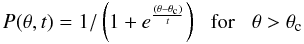 whose limit for small values of the parameter t is the Heaviside step function used before. θc is varied for each value of t to reproduce the observed fractions of HIGs and BLOs. For example, for t = 10°, we derive θc ~ 43° and there is a ~0.9% probability to have a clear view of the nucleus for an object seen along the torus equator, P90. The results for t = 3° are θc ~ 47° and P90 ~ 7 × 10⁻⁷.
The values of P90 obtained for t = 10° and 3°, corresponds to a number of clumps along the line of sight of  , respectively (Natta & Panagia 1984), assuming the torus as a thick inhomogeneous dust layer in front of an extended emitting source. According to the analysis of Nenkova et al. (2008), this is the range in the number of dusty clouds along radial equatorial rays that accounts for the AGN infrared observations. From this simple approach, we conclude that the torus critical angle changes only slightly in case the torus has a clumpy structure. We will show that this has no significant effects on the results obtained in the following sections.
 |
Fig. 3 Probability distribution adopted to simulate the effect of a clumpy torus. P is the probability of an AGN seen at angle θ (in degrees) to be classified as a BLO. The various curves corresponds to t = 0.01° (solid red), 3° (dotted green), 10° (dashed blue), and 30° (dot dashed black), see text. θc is the “knee” angle where the probability drastically changes slope. |
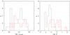 |
Fig. 4 Histograms comparing the distribution of the 178 MHz radio luminosity in erg s-1 Hz-1 units (left) and core dominance R (right) for HIGs (solid black) and BLOs (dashed red). R is the ratio between the total radio luminosity at 178 MHz and the core power at 5 GHz. |
Radio properties of HIGs and BLOs.
5. Radio properties and the unified model
Several tests for the validity of the UM are based on the radio properties of the objects considered. The basic requirement is that the distribution of extended/low-frequency radio power of the two AGN classes considered do not differ. This is met by the 3CR sample. Indeed, from the point of view of their radio power, the average values of L178 MHz of the BLOs and HIGs classes differ by only 0.18 dex and their median by −0.09 dex (see Table 3 and Fig. 4) and also the spread of these distributions are very similar (0.57 dex for HIG, 0.49 dex for BLO). We verified through a Kolmogorov-Smirnov (KS) test that the two populations are not different at a statistical significance level greater than 90%.
According to the UM, the core dominance (defined as the ratio between the core power at 5 GHz and the total luminosity at 178 MHz, i.e., R = Pcore/L178 MHz) should be larger in BLOs than in HIGs, because BLOs are seen at smaller angles with respect to the jet direction than HIGs. This produces a stronger relativistic Doppler boosting of the jet emission in BLOs, causing their radio cores to be relatively brighter. Since the extended radio emission is isotropic, only Pcore could suffer from beaming effects. Thus the core dominance R = Pcore/L178 MHz is a good estimator of beaming and orientation. This effect also provides us with a tool to explore the jet properties in these radio sources.
The intensity of the core emission is enhanced, with respect to its intrinsic value, I0, as I = I0δp + α where δ is the relativistic Doppler factor. δ depends on the velocity of the jet (v = βc) and on the angle θ formed with our line of sight as δ = Γ-1(1 − βcosθ)-1, where Γ = (1 − β2)− 1/2 is the bulk Lorentz factor of the jet, α is the spectral index in the band considered (α ~ 0 for the radio core); p instead depends on the structure of the emitting region (p = 2 for a cylindrical jet and p = 3 for a single emitting blob, see Urry & Padovani 1995).
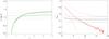 |
Fig. 5 Results of Monte Carlo simulations to derive the jet Lorentz factor Γ and the intrinsic spread of core dominance σintr. The left panel shows the core dominance difference, Δlog R, of a simulated sample of HIGs and BLOs as a function of Γ. The black solid curve is for the average value, while the green line is for the median. The horizontal lines show the observed values, with the dashed lines representing the errors. Right panel: curves of the intrinsic spread of core dominance, σintr, required to reproduced the observed values of the widths of the core dominance distributions for HIGs (black) and BLOs (red) as a function of Γ. At the intercept the constraints for HIGs and BLOs are simultaneously satisfied. The dashed lines for each class are obtained by considering the errors on the dispersions. |
We left out from the analysis three objects (namely, 3C 93.1, 3C 180, and 3C 458) because they do not have a 5 GHz radio core measurement in the literature, leaving us with 48 objects.
The presence of beaming effects on the radio core is clearly shown by the histograms of core dominance, see Fig. 4 (left panel). The median of log R is −3.20 and −1.97 for HIGs and BLOs, respectively (the average values are instead −3.22 and −2.13, respectively) and thus they differ by more than a factor of 10 (Table 3). A KS test indicates that the two populations are different at a level of confidence of >99%.
The R distributions for HIGs and BLOs are directly associated with the jet properties. For example, the higher is Γ, the largest is the difference in core dominance between the two classes. In the following we use the observational information on the core dominance to constrain the jet properties of FR II radio galaxies with high-ionization optical spectra.
We start running a Monte Carlo simulation to study the relation between Γ and the separations between the core dominance distributions of HIGs and BLOs. Operatively, we extract 100 000 objects oriented at a random angle in the plane of the sky considering the case of a cylindrical emitting region (p = 2). Using a torus angle of 50°, as estimated above, we derive the moments of the resulting core dominance distributions of HIGs and BLOs at varying the jet Lorentz factor. In the left panel of Fig. 5, we consider the differences in the average R between BLOs and HIGs. The observed value of Δlog R = 1.09 ± 0.21 is reproduced for  . By using the observed difference of the median, we obtain Γ ≳ 2.8. By considering the possibility of a clumpy torus, these results change only marginally: for t = 10° we obtained a slightly higher value, i.e., Γ ~ 4.0.
We then modeled the spreads of the core dominance distributions, σR. These depend not only on Γ but also on the presence of an intrinsic difference in the core dominance among the various sources. We assumed that the intrinsic distribution is described by a logarithmic gaussian of width σintr and ran a Monte Carlo simulation. For each value of Γ we derived the corresponding value of σintr that reproduces the observed values of σR (0.50 for HIGs and 0.81 for BLOs). With this procedure we obtain the curves (black for HIGs, red for BLOs) shown in Fig. 5 (right panel). At the location of the intercept (Γ = 7.2 and σintr = 0.43) the constraints for HIGs and BLOs are simultaneously satisfied. Considering the errors on σR, we found 4.4 < Γ < 18 and 0.35 < σintr < 0.51.
These simulations, although instructive, do not completely exploit the available observational data, i.e., the full distributions of core dominance for the two classes. We then proceeded to a further simulation, extracting randomly oriented samples of 48 objects (30 HIGs and 18 BLOs) and estimating the differences between each pair of the ordered lists of observed and simulated core dominance. We varied three parameters: the Γ factor, the intrinsic spread of core dominance, σintr, and, in addition to the previous discussion, also the intrinsic value of the core dominance, Rintr. For each set of free parameters, the procedure is repeated 10 000 times, deriving the average value of the sum of the offsets squared. The best fit corresponds to the set of parameters that returns the minimum average value and it is obtained for  ,
,  ,
,  . The uncertainties have been estimated considering the range of the parameters for which the χ2 value increases by 3.5 2.
We repeated the analysis adopting p = 3 and obtained  ,
,  ,
,  .
.
6. Size of the radio sources and the UM
In addition to the information on the total and core luminosities, the radio emission provides us with a further test on the UM. If the HIGs and the BLOs are two sub-samples of intrinsically identical sources, differing only for their orientation, this should affect the size distribution of the two classes. HIGs, being observed closer to the plane of the sky, should appear larger than BLOs. The distributions of sizes of the two classes, derived from literature images, are shown in Fig. 6. Both are very broad, with most objects having sizes in the range 30 and 600 kpc. A KS test indicates that the linear sizes of the two populations are not statistically different at a >90% level.
Having derived the critical viewing angle that separates HIGs from BLOs, θc ~ 50°, we can estimate the expected ratio between the sizes of the two populations. The ratio between the median sizes of HIGs and BLOs is expected to be 1.7. The observed median values are  kpc and
  kpc for HIGs and BLOs, respectively. However, the uncertainties on these values are rather large, 0.13 and 0.17 dex for the two groups, respectively, corresponding to a poorly constrained ratio of the medians of
  .
.
Thus, the test based on the radio sources on the UM is not conclusive since the size distribution is dominated by the intrinsic scatter rather than by the projection effects.
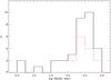 |
Fig. 6 Size distribution (in kpc) of the radio sources associated with HIGs (black histogram) and BLOs (red histogram). |
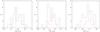 |
Fig. 7 Histograms comparing the luminosity of HIGs (solid black) and BLOs (dashed red) in three narrow emission lines, from left to right, [O III], [O II], and [O I], all in erg s-1 units. |
7. Narrow lines properties
In Buttiglione et al. (2010) we found that HIGs and BLOs lie in the same regions of the optical spectroscopic diagnostic diagrams, indicating that they share similar values of the main emission lines ratios. However, looking at the diagrams in detail, we noticed that BLOs have relatively stronger [O I] line, by an average factor of ~2, than those of HIGs. We then explore this issue in more depth by comparing the luminosity distributions of 3 brightest oxygen optical emission lines, namely [O III], [O II], and [O I], in HIGs and BLOs (see Fig. 7).
The median of the [O III] and [O I] distributions of the two classes differ by a factor ~2 (see Table 4). A KS test indicates that the two populations differ in L[O III] and L[O I] at a statistical significance level greater than 95%. Conversely, looking at the [O II] line, the moments of the distributions differ only marginally and the differences in their cumulative distributions are not statistically significative.
A similar result was already found by Lawrence (1991) who noted that the [O III] luminosity of narrow-lined objects was lower than in broad-lined objects at the same radio power. They observe this effect for various AGN samples selected in optical, infrared, X-ray, and radio band. Furthermore, Hes et al. (1993) found for 3C radio galaxies that the [O II] luminosities do not differ for narrow and broad-lined objects, again in agreement with our results.
These findings can be still accommodated within the UM by assuming that the NLR is partially obscured by the torus. The result that, beside the known difference in [O III], as well as the [O I] luminosities, differ between HIGs and BLOs, suggests that this might be due to a NLR density stratification (rather than to an ionization stratification). Indeed, the three lines considered are associated with different critical densities, with the [O II] lines having the lowest value3. It can be envisaged that approximately half of the [O III] and [O I] emission is produced in a compact, high density region (with a density exceeding the [O II] critical density, i.e., ≳103 cm-3) located within the walls of the obscuring torus.
In line with this scenario, other NLR properties should differ between BLOs and HIGs. In particular the widths of narrow lines of higher critical densities should be broader in BLOs since they have a larger contribution from emission originating closer to the central black hole. This can be tested by measuring the line widths of the three oxygen lines. The spectral resolution of the TNG data obtained for this survey is not suited for such an analysis. We then limit ourselves to the 14 sources (7 BLOs and 7 HIGs) with available SDSS spectra. The velocity widths derived from a single gaussian fit to the lines are shown in Fig. 8. Although the number of sources is rather limited, we find tentative evidence that indeed BLOs have broader [O I] and [O III] lines with respect to HIGs of similar [O II] width. This supports the idea of a radial density gradient in the NLR.
HIGs and BLOs narrow lines distributions.
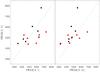 |
Fig. 8 Comparison of the widths (in km s-1) of three oxygen emission lines measured from the available 14 SDSS spectra. BLOs are the red circles, HIGs are represented by the black squares. |
Sample of the 3CR FR II/LIGs with z < 0.3.
8. Low ionization galaxies and the unified model
Until now, we only considered radio sources characterized by emission lines of high ionization, that represent less than half of the 3CR sample up to z = 0.3. However, the study of HIGs and BLOs provides us with a useful benchmark to explore the properties of the other main spectroscopic class of sources in the sample, i.e., the LIGs. While many LIGs have a FR I radio morphology, our spectroscopic study confirms the presence of a significant number of LIGs (21, see Table 5) with a clear FR II structure, despite our rather strict criteria for the definition of the FR type.
The radio properties of FR II/LIGs are generally similar to those of HIGs and BLOs. Beside the morphology, they cover the same range of radio power and also have a similar distribution of core dominance (Buttiglione et al. 2010). The questions that arise are: which is the link between low and high ionization galaxies? Which role do LIGs play in the UM? How do the properties of the LIGs jets compare with those of HIGs and BLOs? We already know from previous studies (e.g., Laing et al. 1994) that the core dominance distribution of 3CR FR II LIGs indicates a randomly-oriented population, different from the HIGs. Therefore, the study of the complete 3CR sample, precisely its LIG sub-sample, can return more solid results on such questions.
First of all, we tested with a KS test that the distributions of radio power of LIGs and HIGs/BLOs are not statistical different (see Fig. 9, left panel). This leaves open the possibility that LIGs might represent a third group of radio sources, part of the same unification scheme with BLOs and HIGs. Furthermore, in the light of the results of the previous section, the differences in optical line ratios between LIGs and HIGs might be due to selective obscuration. For example, LIGs might be seen along a line of sight close to the equatorial plane of the torus, causing the obscuration of a substantial fraction of their NLR. This might account for the factor of ~10 deficit in their [O III] line with respect to HIGs and BLOs (Buttiglione et al. 2010) and also for the differences in line ratios. The optical spectra of FR II/LIGs never show the presence of a significant BLR, and this also would be naturally explained if they are all observed at large θ.
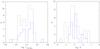 |
Fig. 9 Comparison of the distributions of total radio luminosity at 178 MHz (left) and of the core dominance R (right) for FR II/LIGs (dashed blue) and HIGs+BLOs (solid black). |
In this framework, the UM provides a clear prediction of the radio properties of LIGs: they must show a lower core dominance and a narrower distribution of R, than those of HIGs. But this is not the case: the distribution of R for LIGs has a median value of log R = −2.84 and a spread of 0.70 dex, substantially larger than in HIGs (for which log R = −3.20 and σR = 0.57). Thus LIGs cannot be objects intrinsically identical to HIGs and BLOs just seen at larger viewing angles. In addition, the distribution of core dominance of LIGs is instead not statistically distinguishable from the distribution of the population formed by HIGs plus BLOs (see also Fig. 9, right panel) at a 90% level.
Since broad lines are intrinsically absent in LIG spectra, no indications on orientation can be obtained from their optical spectra. To explore their properties, we must rely only on their radio properties. Following the analysis described in Sect. 5, we modeled the distribution of R in LIGs and we derived the following set of parameters: Γ < 3.25, σintr < 0.74,  for p = 2 4. Due to the small number of objects, the constraints on the jet’s parameters in LIGs are rather weak.
9. Discussion
The complete 3CR optical survey allows us to derive more accurate results than in previous works in the framework of testing the predictions of the UM for FR II radio sources, when high and low ionization objects are properly separated. In particular, the 3CR HIGs and BLOs, limited at z < 0.3, show differences and similarities in the radio and line-emission properties which are ascribable to a random orientation of the parent population, fundamental requirement of the UM.
A key element in the UM is the presence of a circumnuclear structure that hides the view of the innermost regions of the AGN in the optical band when seen at large angle from its axis. Our spectroscopic survey clearly cannot provide any direct evidence for the existence of an obscuring torus. However, the connection between the radio core dominance and the optical spectra (i.e., to the presence/absence of broad emission lines), confirms the link between orientation of the AGN and its spectral classification, requiring the presence of an absorbing structure.
In the assumption that the torus is present in FR II-type radio-loud AGN, we can obtain information on its geometric structure. The simple torus geometry we assumed provides an estimate of its opening angle θc = 50° ± 5. Although the sample is limited to z = 0.3, there is not evidence of change of the torus angle throughout the redshift and luminosity range of the sample. Furthermore, Barthel (1989) selected a sample of ~50 quasars and radio galaxies in the 3C catalog with 0.5 < z < 1.0 with a radio power in the range L178 MHz ~ 1035 − 1036 erg s-1 Hz-1. He derived a value of θc , in agreement with our estimate. This further supports our conclusion that the torus geometry does not vary significantly with radio power over ~3 orders of magnitudes. This contrasts with the “receding torus” model proposed by Lawrence (1991) and Hill et al. (1996) who find a decreasing fraction of broad and narrow line objects in the 3CR at increasing radio luminosity. Nevertheless, the problem is far to be solved since there are conflicting results in literature. In fact, another study on 3CR radio sources which compares objects at z < 0.3 with others to z ~ 1 returns that the covering factor of the obscuring structure decreases as the redshift increases (Varano et al. 2004). The solution might be reached with large samples which cover wide range of luminosities and redshifts. In addition, the inclusion of LIGs in the composite sample might strongly affect the results, since they appear to be a different FR II population from HIGs and BLOs.
We also consider the possibility of a clumpy structure for the torus. This allows us to see directly the nuclear regions according to an arbitrary probabilistic law, that is not null even along the torus equator. Limiting to a level of torus porosity allowed by the infrared observations of AGN, we find that the torus opening angle might decrease only slightly, to ~43°, and this has a marginal effect on the estimates of the jet Lorentz factor. However, the question on the nature of the torus is still far from being resolved as suggested by the conflicting results on radiative transfer in clumpy media (e.g., Landt et al. 2010).
The test of the UM based on the radio source size of these 3CR source is instead not conclusive. This is due to the fact that the expected foreshortening of BLOs with respect to HIGs amounts to only a factor of 1.7 and is too small to be appreciated in the observed size distribution dominated by the intrinsic scatter. This effect should be derived by comparing two intrinsic size distributions that are very broad, ranging from ~30 to ~600 kpc, leading to an error of the median sizes of the two classes of a factor of ~3. Only a substantially larger number of objects might unveil a genuine difference in size between HIGs and BLOs. The absence of this foreshortening of the sizes of quasars as compared to those of radio galaxies of similar flux densities or at similar (low and high) redshifts has been observed in larger samples (e.g. Boroson 2011, in prep.; Singal & Laxmi Singh 2013). A possible reason of this conflict with what expected from the UM can be ascribed to the presence of LIG in those large sample which do not participate in orientation unification schemes as explicitly discussed by Singal & Laxmi Singh (2013). DiPompeo et al. (2013) underlines the importance of considering the intrinsic size distribution of radio sources in this context. They found that, while it is possible to reconcile conflicting results purely within a simple, orientation-based framework, it is very unlikely.
Adopting the UM model, it is possible to constrain the jet properties needed to reproduce the observed distributions of radio core dominance in HIGs and BLOs. We find that this is obtained for a jet bulk Lorentz factor in the range Γ ~ 3−5 (for p = 2), nearly independent on the torus properties. A comparison with previous results on the jet bulk Lorentz factor for radio galaxies is necessary. Padovani & Urry (1991) derived an estimate of Γo in the optical band comparing the number density of BL Lac objects and the parent population of FR I galaxies, by combining a correction for the effect of beaming and contamination from the host galaxy on the optical luminosity function. They found 8 < Γo < 20, a larger range than the Lorentz factor inferred for the X-ray emitting plasma ΓX ~ 3 (Padovani & Urry 1990) and roughly of the same order of the radio Lorentz factor, 5 ≲ Γr ≲ 35 (Urry et al. 1991). Studies on the Chandra X-ray jets for FR II radio galaxies provides measurements of the bulk Lorentz factor in the range 2−7 (Hardcastle et al. 2002; Siemiginowska et al. 2003; Hogan et al. 2011). Whereas the previous estimates of the bulk Lorentz factors are derived from luminosity functions or emission models, Hardcastle et al. (1999) takes in account the information of the angle orientation from the optical spectroscopic classification (into HIGs and BLOs) for a sample of FR IIs, excluding LIGs. By modeling the distributions of jet prominence of the sample, they derive a bulk Lorentz factor of ~5. Conversely, there are no proper measurements of Γ for a sample of FR II LIGs in the literature.
The Lorentz factors inferred from the apparent superluminal jet motions (up to γ ~ 30, see review from Kellermann et al. 2007), are substantially larger than our values. This issue was already argument of debate since the dynamic range of core dominances expected from superluminal motions predicts a much larger number of debeamed sources than what obtained from observations. This inconsistency can be ascribed to the simplistic assumption of a cylindrical jet model without any internal velocity structure. This does not conform to some jet features, such as jet bending (e.g., Readhead et al. 1983). Instead, the inclusion of shock waves in the hydrodynamic models seems to better reconcile with the observations (Blandford 1984; Lind & Blandford 1985). This result is reminiscent of what is found from the comparison of the properties of FR I radiogalaxies and BL Lacs (Chiaberge et al. 2000). Summarizing, the derivations of the bulk velocity of the relativistic jets in different bands and with approaches appear to be approximatively consistent with each other, even though the sources show different radio morphologies (FR I and FR II) and nuclear properties (HIGs and LIGs).
Another key test of the UM is based on the properties of NLRs: they are structures extending out to a scale of several kpc and thence they are thought generally to be unaffected by nuclear obscuration. For this reason the luminosity of the narrow emission lines apparently represents an isotropic quantity, particularly useful when testing the UM. Instead, thanks to the completeness of the spectroscopic data we found evident discrepancies in terms of properties of the three brightest oxygen optical emission line ([O III], [O II], and [O I]) between HIGs and BLOs. Such differences are not in agreement with the UM at the zeroth-order approximation, which predicts similar NLR properties. However, our results can be accommodated within the UM, if we assume a partial obscuration by the torus on the nuclear region of the NLR. Furthermore, the luminosity distribution and the FWHM of the oxygen lines return an interesting result: they invoke a NLR density stratification, where an innermost region, compact and dense, is responsible to produce approximately half of the [O I] and [O III] emission lines. Their higher critical densities with respect to the [O II] might account for a higher spatial concentration closer to the black hole. This region appears to be a crucial component of the NLR, apparently confined to a scale on the order of the dust sublimation radius (i.e., pc scale, Barvainis 1987), larger but comparable to the BLR radius (Bentz et al. 2013). It is tempting to associate it with the walls of the torus, indeed rich of dense neutral gas, producing the observed large amount of high velocity [O I] emission. Its density is sufficiently low to allow the production of narrow lines, and thence lower than in the BLR, but some of them are already strongly depressed by collisional de-excitation. Furthermore, in agreement with our partially obscured NLR model, spectro-polarimetric data show evidences of a prominent contribution from scattered [O III] lines, emitted behind this obscuring material (di Serego Alighieri et al. 1997; Cohen et al. 1999).
This applies not only to radio-loud AGN, but also to radio-quiet objects. In fact previous studies (Lawrence 1987; Gaskell 1984; Zhang et al. 2008; Gaskell 2009) show emission line differences between type 1 and type 2 AGN similar to the 3CR BLOs and HIGs. Direct evidence for a compact and dense NLR component comes from the detection of variability of the [O III] flux in NGC 5548 over a timescale of a few years (Peterson et al. 2013); they derived a size of a few pc and an electronic density of ~105 cm-3. A similar structure is also seen around the nuclei in FR I radio galaxies from the analysis of HST spectra and narrow-band images (Capetti et al. 2005).
Finally, the study of the radio and core dominance distribution of 3CR FR II LIGs indicates that they do not have a preferred orientation in the plane of the sky, supporting the results of Laing et al. (1994). In this case, broad lines are intrinsically missing in LIGs, at odds with what is seen in the BLOs/HIGs class, and similarly to the indications obtained for the FR I/LIGs (e.g., Chiaberge et al. 1999; Baldi et al. 2010).
The differences between low and high ionization radio galaxies cannot be just due to orientation but they are intrinsically different objects at the nuclear scales. Their different properties reflect the bimodality of accretion modes in RL AGN population. While HIGs/BLOs show thermal nuclei characteristic of “standard” accretion mode, LIGs appear to have synchrotron-dominated nuclei powered by radiatively inefficient accretion disk (e.g., Chiaberge et al. 2002; Hardcastle et al. 2006; Baldi et al. 2010). The infrared emission is crucial to unveil the presence of a hidden quasar and separate the two AGN classes; this spectral band acts as a calorimeter in which a large fraction of the AGN bolometric power is reprocessed (see the review on this topic by Antonucci 2012).
10. Summary and conclusions
The complete optical spectroscopic survey for 3CR sources with z < 0.3 (Buttiglione et al. 2010) provides us with a homogenous sample perfectly suited to test various predictions and discuss the implications of the UM for FR II radio galaxies. We exclusively consider the FR II HIG sample which consists of 33 narrow line objects and 18 broad-lined objects (BLOs). The aim is to derive the main quantities involved in the UM for RL AGN: the opening angle of the obscuring torus and the bulk Lorentz factor of the relativistic jets. The method used is the study of the core dominance distribution of the sample and their emission line properties. The main results are summarized as follows:
-
The HIGs/BLOs number ratio corresponds to an opening angle of an obscuring torus of θc= 50° ± 5°. There is no evidence of a dependence of this value with redshift/luminosity within the sample considered, up to z = 0.3.
-
While HIGs and BLOs share the distribution of total radio luminosity, their core dominance distributions are significantly offset, by ~1 order of magnitude. This implies that it exists a strong link between the optical and radio properties, with the jets in BLOs forming an angle with the line of sight smaller than HIGs, supporting the validity of the UM. We modeled the distributions of R to estimate the jet bulk Lorentz factor, obtaining Γ ~ 3 − 5.
-
We consider the possibility of a “clumpy” torus: this has only a small impact on its “opening angle” and on the value of Γ.
-
The test of the UM based on the radio source size is not conclusive, due to the small number of objects considered.
-
While the properties of the [O II] emission line are similar in BLOs and HIGs, they differ for the [O III] and [O I] lines. In particular, these lines are broader and more luminous in BLOs. This is consistent with a combination of obscuration and density stratification in the NLR. Approximately half of the line emitting gas (with high critical density, i.e. [O I] and [O III]) is located within the walls of the obscuring torus and it is visible only in BLOs, while it is obscured in HIGs.
-
Considering now the FR II LIGs, they might be, in principle, all objects seen at high inclination, with the BLR and also most of the NLR hidden from our view. This is incompatible with their broad core dominance distribution that is instead consistent with what is expected from a sample of random oriented sources. Thus LIGs can not belong to the same UM with HIGs and BLOs. This result lends further support to the idea that LIGs constitute a separate class of radio-loud AGN, as already suggested by the differences in their nuclear properties. Unfortunately, due to the limited number of LIGs, we cannot perform a robust comparison between the jet Lorentz factor of the different classes of radio sources. Thence we are not able to conclude whether there is an association between the jet properties (and the jet launching mechanism) and the different spectral types.
Overall, the results obtained for FR II radio sources are consistent with a pure orientation-based unified model, when considering separately objects of high and low ionization. Indeed, we find that the distributions of total radio luminosity of HIGs and BLOs are not statistically distinguishable, while BLOs have a higher radio core dominance than HIGs. This links the orientation indicator based on the radio data with the effects of selective nuclear obscuration, as expected in the UM framework.
We find significant differences in the properties of narrow emission lines between HIGs and BLOs, but this does not contrast with the UM even in its simplest version. While historically the narrow lines have been considered isotropic, there is mounting evidence that a significant fraction of the emission from forbidden lines originates from a compact and dense region located within the walls of the torus. This is visible only in type 1 AGN, i.e. in the BLOs, and it is not exclusively associated to radio-loud objects, being present also in radio-quiet AGN.
Online material
Main properties of the sample of HIGs and BLOs with z < 0.3 in the 3CR catalog.
We adopt the HIG/LIG nomenclature that better represents the separation of the two classes based on the ionization conditions in the narrow-line region gas in these objects. This classification is however entirely consistent with the HEG/LEG scheme (high/low excitation galaxies) widely adopted in the literature.
This value corresponds to the amount that the χ2 is allowed to increase for a confidence level of 68% and for three free parameters.
The logarithms of critical densities, in cm-3 units, are ~3.5, 2.8, 5.8, and 6.3 for [O II]λ3726, [O II]λ3729, [O III]λ5007, and [O I]λ6300, respectively (Appenzeller & Oestreicher 1988).
For p = 3 we find Γ < 1.90, σintr < 0.70,  .
.
Acknowledgments
R.D.B. acknowledges the financial support from SISSA, Trieste. We are grateful to the referee R. Antonucci for the extremely useful comments to improve the paper. This work is primarly based on observations made with the Italian Telescopio Nazionale Galileo of INAF (Istituto Nazionale di Astrofisica) at the Spanish Observatorio del Roque del los Muchachos of the Instituto de Astrofisica de Canarias.
References
- Antonucci, R. 1993, ARA&A, 31, 473 [Google Scholar]
- Antonucci, R. 2012, Astron. Astrophys. Trans., 27, 557 [NASA ADS] [Google Scholar]
- Antonucci, R. R. J. 1982, Nature, 299, 605 [NASA ADS] [CrossRef] [Google Scholar]
- Antonucci, R. R. J. 1984, ApJ, 278, 499 [NASA ADS] [CrossRef] [Google Scholar]
- Appenzeller, I., & Oestreicher, R. 1988, AJ, 95, 45 [NASA ADS] [CrossRef] [Google Scholar]
- Baldi, R. D., Chiaberge, M., Capetti, A., et al. 2010, ApJ, 725, 2426 [NASA ADS] [CrossRef] [Google Scholar]
- Barthel, P. D. 1989, ApJ, 336, 606 [Google Scholar]
- Barvainis, R. 1987, ApJ, 320, 537 [NASA ADS] [CrossRef] [Google Scholar]
- Bennett, A. S. 1962a, MNRAS, 125, 75 [NASA ADS] [Google Scholar]
- Bennett, A. S. 1962b, MmRAS, 68, 163 [Google Scholar]
- Bentz, M. C., Denney, K. D., Grier, C. J., et al. 2013, ApJ, 767, 149 [NASA ADS] [CrossRef] [Google Scholar]
- Bevington, P. R., & Robinson, D. K. 2003, Data reduction and error analysis for the physical sciences (Boston: McGraw-Hill) [Google Scholar]
- Blandford, R. D. 1984, in VLBI and Compact Radio Sources, eds. R. Fanti, K. I. Kellermann, & G. Setti, IAU Symp., 110, 215 [Google Scholar]
- Boroson, T. A. 2011, in American Astronomical Society Meeting Abstracts, BAAS, 43, 142.22 [Google Scholar]
- Buttiglione, S., Capetti, A., Celotti, A., et al. 2009, A&A, 495, 1033 [NASA ADS] [CrossRef] [EDP Sciences] [Google Scholar]
- Buttiglione, S., Capetti, A., Celotti, A., et al. 2010, A&A, 509, A6 [NASA ADS] [CrossRef] [EDP Sciences] [Google Scholar]
- Buttiglione, S., Capetti, A., Celotti, A., et al. 2011, A&A, 525, A28 [NASA ADS] [CrossRef] [EDP Sciences] [Google Scholar]
- Capetti, A., Verdoes Kleijn, G., & Chiaberge, M. 2005, A&A, 439, 935 [NASA ADS] [CrossRef] [EDP Sciences] [Google Scholar]
- Capetti, A., Raiteri, C. M., & Buttiglione, S. 2010, A&A, 516, A59 [NASA ADS] [CrossRef] [EDP Sciences] [Google Scholar]
- Chiaberge, M., Capetti, A., & Celotti, A. 1999, A&A, 349, 77 [NASA ADS] [Google Scholar]
- Chiaberge, M., Capetti, A., & Celotti, A. 2000, A&A, 355, 873 [NASA ADS] [Google Scholar]
- Chiaberge, M., Capetti, A., & Celotti, A. 2002, A&A, 394, 791 [NASA ADS] [CrossRef] [EDP Sciences] [Google Scholar]
- Cohen, M. H., Ogle, P. M., Tran, H. D., Goodrich, R. W., & Miller, J. S. 1999, AJ, 118, 1963 [NASA ADS] [CrossRef] [Google Scholar]
- DiPompeo, M. A., Runnoe, J. C., Myers, A. D., & Boroson, T. A. 2013, ApJ, 774, 24 [NASA ADS] [CrossRef] [Google Scholar]
- di Serego Alighieri, S., Cimatti, A., Fosbury, R. A. E., & Hes, R. 1997, A&A, 328, 510 [NASA ADS] [Google Scholar]
- Fanaroff, B. L., & Riley, J. M. 1974, MNRAS, 167, 31P [Google Scholar]
- Gaskell, C. M. 1984, Astrophys. Lett., 24, 43 [NASA ADS] [Google Scholar]
- Gaskell, C. M. 2009, ArXiv e-prints [Google Scholar]
- Hardcastle, M. J., Alexander, P., Pooley, G. G., & Riley, J. M. 1999, MNRAS, 304, 135 [NASA ADS] [CrossRef] [Google Scholar]
- Hardcastle, M. J., Birkinshaw, M., Cameron, R. A., et al. 2002, ApJ, 581, 948 [NASA ADS] [CrossRef] [Google Scholar]
- Hardcastle, M. J., Evans, D. A., & Croston, J. H. 2006, MNRAS, 370, 1893 [NASA ADS] [CrossRef] [Google Scholar]
- Hes, R., Barthel, P. D., & Fosbury, R. A. E. 1993, Nature, 362, 326 [NASA ADS] [CrossRef] [Google Scholar]
- Hill, G. J., Goodrich, R. W., & Depoy, D. L. 1996, ApJ, 462, 163 [NASA ADS] [CrossRef] [Google Scholar]
- Hine, R. G., & Longair, M. S. 1979, MNRAS, 188, 111 [NASA ADS] [Google Scholar]
- Hogan, B. S., Lister, M. L., Kharb, P., Marshall, H. L., & Cooper, N. J. 2011, ApJ, 730, 92 [NASA ADS] [CrossRef] [Google Scholar]
- Jackson, C. A., & Wall, J. V. 1999, MNRAS, 304, 160 [NASA ADS] [CrossRef] [Google Scholar]
- Jackson, N., & Rawlings, S. 1997, MNRAS, 286, 241 [NASA ADS] [CrossRef] [Google Scholar]
- Kellermann, K. I., Kovalev, Y. Y., Lister, M. L., et al. 2007, Ap&SS, 311, 231 [NASA ADS] [CrossRef] [Google Scholar]
- Laing, R. A., Jenkins, C. R., Wall, J. V., & Unger, S. W. 1994, in The First Stromlo Symposium: The Physics of Active Galaxies, eds. G. V. Bicknell, M. A. Dopita, & P. J. Quinn, ASP Conf. Ser., 54, 201 [Google Scholar]
- Landt, H., Buchanan, C. L., & Barmby, P. 2010, MNRAS, 408, 1982 [NASA ADS] [CrossRef] [Google Scholar]
- Lawrence, A. 1987, PASP, 99, 309 [NASA ADS] [CrossRef] [Google Scholar]
- Lawrence, A. 1991, MNRAS, 252, 586 [NASA ADS] [Google Scholar]
- Lind, K. R., & Blandford, R. D. 1985, ApJ, 295, 358 [NASA ADS] [CrossRef] [Google Scholar]
- Natta, A., & Panagia, N. 1984, ApJ, 287, 228 [NASA ADS] [CrossRef] [Google Scholar]
- Nenkova, M., Sirocky, M. M., Nikutta, R., Ivezić, Ž., & Elitzur, M. 2008, ApJ, 685, 160 [NASA ADS] [CrossRef] [Google Scholar]
- Padovani, P., & Urry, C. M. 1990, ApJ, 356, 75 [NASA ADS] [CrossRef] [Google Scholar]
- Padovani, P., & Urry, C. M. 1991, ApJ, 368, 373 [NASA ADS] [CrossRef] [Google Scholar]
- Peterson, B. M., Denney, K. D., De Rosa, G., et al. 2013, ApJ, submitted [arXiv:1309.1468] [Google Scholar]
- Readhead, A. C. S., Hough, D. H., Ewing, M. S., Walker, R. C., & Romney, J. D. 1983, ApJ, 265, 107 [NASA ADS] [CrossRef] [Google Scholar]
- Siemiginowska, A., Stanghellini, C., Brunetti, G., et al. 2003, ApJ, 595, 643 [NASA ADS] [CrossRef] [Google Scholar]
- Singal, A. K., & Laxmi Singh, R. 2013, ApJ, 766, 37 [NASA ADS] [CrossRef] [Google Scholar]
- Spinrad, H., Marr, J., Aguilar, L., & Djorgovski, S. 1985, PASP, 97, 932 [NASA ADS] [CrossRef] [Google Scholar]
- Urry, C. M., & Padovani, P. 1995, PASP, 107, 803 [NASA ADS] [CrossRef] [Google Scholar]
- Urry, C. M., Padovani, P., & Stickel, M. 1991, ApJ, 382, 501 [NASA ADS] [CrossRef] [Google Scholar]
- Varano, S., Chiaberge, M., Macchetto, F. D., & Capetti, A. 2004, A&A, 428, 401 [NASA ADS] [CrossRef] [EDP Sciences] [Google Scholar]
- Wall, J. V., & Jackson, C. A. 1997, MNRAS, 290, L17 [NASA ADS] [CrossRef] [Google Scholar]
- Zhang, K., Wang, T., Dong, X., & Lu, H. 2008, ApJ, 685, L109 [NASA ADS] [CrossRef] [Google Scholar]
Appendix A: Estimate of the orientation of a radio source based on the core dominance
One interesting application of the derivation of the radio parameters (jet bulk Lorentz factor Γ, intrinsic core dominance Rintr, and intrinsic spread of the core dominance distribution σintr) from the core dominance distribution of 3CR/FR II radio galaxies (HIGs and BLOs) is the possibility of estimating their orientation starting from the measurement of the core dominance of individual objects. By inverting the link between the core dominance R and the viewing angle θ the analytical relation is the following:
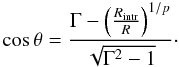 In Fig. A.1 we show the two curves obtained for p = 2 and p = 3 and adopting the jet’s parameters derived in Sect. 5. We also show the curves obtained by considering the errors on the three parameters (see Sect. 5). For example, for a radio source with a core dominance logR = −2 we derive θ = 20° ± 8°.
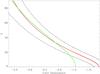 |
Fig. A.1 Orientation angle vs. core dominance relation obtained by using the derived three parameters (jet bulk Lorentz factor Γ, intrinsic core dominance Rintr, and intrinsic spread of the core dominance distribution σintr) for HIG and BLO from their core dominance distribution. The red curve is for p = 2 (cylindrical jet) with the error curves represented by the dashed line. The green curve is for p = 3 (single emitting blob). |
A possible application of such relations is the deprojection of a radio source and the estimate of its real size.
All Tables
All Figures
|
Fig. 1 Left panel: fit to the spectrum of 3C 133 obtained by forcing the presence of a broad Hα. Right panel: result of the fit with only narrow line components. The original spectrum is in black, the narrow lines are in green, and the broad Hα is in blue. The residuals are shown in the top panel of both figures. |
| In the text | |
|
Fig. 2 Comparison between the narrow [O III] line and the broad Hα fluxes. Red squares are BLOs, black circles are HIGs, with empty symbols representing upper limits. The fluxes are in erg cm-2 s-1. The solid line marks the average ratio between the two emission lines as measured in BLOs, (FHα broad/F[O III] ~ 8). The dashed lines illustrate a change of a factor of 4 in this value. |
| In the text | |
|
Fig. 3 Probability distribution adopted to simulate the effect of a clumpy torus. P is the probability of an AGN seen at angle θ (in degrees) to be classified as a BLO. The various curves corresponds to t = 0.01° (solid red), 3° (dotted green), 10° (dashed blue), and 30° (dot dashed black), see text. θc is the “knee” angle where the probability drastically changes slope. |
| In the text | |
|
Fig. 4 Histograms comparing the distribution of the 178 MHz radio luminosity in erg s-1 Hz-1 units (left) and core dominance R (right) for HIGs (solid black) and BLOs (dashed red). R is the ratio between the total radio luminosity at 178 MHz and the core power at 5 GHz. |
| In the text | |
|
Fig. 5 Results of Monte Carlo simulations to derive the jet Lorentz factor Γ and the intrinsic spread of core dominance σintr. The left panel shows the core dominance difference, Δlog R, of a simulated sample of HIGs and BLOs as a function of Γ. The black solid curve is for the average value, while the green line is for the median. The horizontal lines show the observed values, with the dashed lines representing the errors. Right panel: curves of the intrinsic spread of core dominance, σintr, required to reproduced the observed values of the widths of the core dominance distributions for HIGs (black) and BLOs (red) as a function of Γ. At the intercept the constraints for HIGs and BLOs are simultaneously satisfied. The dashed lines for each class are obtained by considering the errors on the dispersions. |
| In the text | |
|
Fig. 6 Size distribution (in kpc) of the radio sources associated with HIGs (black histogram) and BLOs (red histogram). |
| In the text | |
|
Fig. 7 Histograms comparing the luminosity of HIGs (solid black) and BLOs (dashed red) in three narrow emission lines, from left to right, [O III], [O II], and [O I], all in erg s-1 units. |
| In the text | |
|
Fig. 8 Comparison of the widths (in km s-1) of three oxygen emission lines measured from the available 14 SDSS spectra. BLOs are the red circles, HIGs are represented by the black squares. |
| In the text | |
|
Fig. 9 Comparison of the distributions of total radio luminosity at 178 MHz (left) and of the core dominance R (right) for FR II/LIGs (dashed blue) and HIGs+BLOs (solid black). |
| In the text | |
|
Fig. A.1 Orientation angle vs. core dominance relation obtained by using the derived three parameters (jet bulk Lorentz factor Γ, intrinsic core dominance Rintr, and intrinsic spread of the core dominance distribution σintr) for HIG and BLO from their core dominance distribution. The red curve is for p = 2 (cylindrical jet) with the error curves represented by the dashed line. The green curve is for p = 3 (single emitting blob). |
| In the text | |
Current usage metrics show cumulative count of Article Views (full-text article views including HTML views, PDF and ePub downloads, according to the available data) and Abstracts Views on Vision4Press platform.
Data correspond to usage on the plateform after 2015. The current usage metrics is available 48-96 hours after online publication and is updated daily on week days.
Initial download of the metrics may take a while.