| Issue |
A&A
Volume 560, December 2013
|
|
|---|---|---|
| Article Number | A113 | |
| Number of page(s) | 11 | |
| Section | Astronomical instrumentation | |
| DOI | https://doi.org/10.1051/0004-6361/201321894 | |
| Published online | 16 December 2013 | |
FIRST, a fibered aperture masking instrument
II. Spectroscopy of the Capella binary system at the diffraction limit
1
LESIA, Observatoire de Paris, CNRS, UPMC, Université
Paris-Diderot, Paris Sciences et Lettres,
5 place Jules
Janssen
92195
Meudon
France
e-mail:
This email address is being protected from spambots. You need JavaScript enabled to view it.
2
Department of Astronomy, University of California at
Berkeley, Hearst Field Annex,
B-20, Berkeley
CA
94720-3411,
USA
3
UJF-Grenoble 1 / CNRS-INSU, Institut de Planétologie et
d’Astrophysique (IPAG) UMR 5274, 38041
Grenoble,
France
4
Carl Sagan Center at the SETI Institute,
189 Bernardo Av., Mountain View
CA
94043,
USA
5
Extrasolar Planet Detection Project Office, National Astronomical
Observatory of Japan, 2-21-1 Osawa,
Mitaka, 181-8588
Tokyo,
Japan
6
Space Telescope Science Institute, 3700 San Martin Drive, Baltimore, MD
21218,
USA
7
University of California Observatories/Lick
Observatory, PO Box
85, Mount Hamilton,
CA
95140,
USA
8
Gemini Observatory, 670 North A’ohoku Place, Hilo, 96720
Hawaii,
USA
9
Subaru Telescope, 650 North A’ohoku Place,
Hilo, 96720
Hawaii,
USA
10
CRAL UMR 5574: CNRS, Université de Lyon, École Normale Supérieure de Lyon,
46 allée
d’Italie, 69364
Lyon Cedex 7,
France
11
IMCCE, Observatoire de Paris, Avenue Denfert-Rochereau, 75014
Paris,
France
Received: 14 May 2013
Accepted: 25 October 2013
Abstract
Aims. FIRST is a prototype instrument built to demonstrate the capabilities of the pupil remapping technique, using single-mode fibers and working at visible wavelengths. Our immediate objective is to demonstrate the high angular resolution capability of the instrument and to show that the spectral resolution of the instrument enables characterization of stellar companions.
Methods. The FIRST-18 instrument is an improved version of FIRST-9 that simultaneously recombines two sets of nine fibers instead of one, thus greatly enhancing the (u, v) plane coverage. We report on observations of the binary system Capella at three epochs over a period of 14 months (≳4 orbital periods) with FIRST-18 mounted on the 3 m Shane telescope at Lick Observatory. The binary separation during our observations ranges from 0.8 to 1.2 times the diffraction limit of the telescope at the central wavelength of the spectral band.
Results. We successfully resolved the Capella binary system at all epochs, with an astrometric precision as good as 1 mas under the best observing conditions. FIRST also gives access to the spectral flux ratio between the two components directly measured with an unprecedented spectral resolution of R ~ 300 over the 600−850 nm range. In particular, our data allow detection of the well-known overall slope of the flux ratio spectrum, leading to an estimation of the “pivot” wavelength of 0.64 ± 0.01 μm, at which the cooler component becomes the brightest. Spectral features arising from the difference in effective temperature of the two components (specifically the Hα line, TiO, and CN bands) have been used to constrain the stellar parameters. The effective temperatures we derive for both components are slightly lower (5−7%) than the well-established properties for this system. This difference mainly comes from deeper molecular features than those predicted by state-of-the-art stellar atmospheric models, suggesting that molecular line lists used in the photospheric models are incomplete and/or oscillator strengths are underestimated, most likely concerning the CN molecule.
Conclusions. These results demonstrate the power of FIRST, which is a fibered pupil remapping-based instrument, in terms of high angular resolution and show that the direct measurement of the spectral flux ratio provides valuable information to characterize little known companions.
Key words: instrumentation: high angular resolution / techniques: interferometric / binaries: close / binaries: visual / stars: fundamental parameters / stars: individual: Capella
© ESO, 2013
1. Introduction
The objective of the FIRST (Fibered Imager foR a Single Telescope) prototype development is the detection of faint companions such as exoplanets. Many instruments currently being designed and manufactured are addressing this challenge, which requires high dynamic ranges at high angular resolution. Different solutions are implemented, such as extreme adaptive optics systems, coronagraphic masks, and interferometric techniques (or a combination thereof). FIRST belongs to the last category since its principle relies on aperture masking (Haniff et al. 1987), in which a mask with small holes is put on the pupil of the telescope. In a traditional implementation, these holes are organized in a non-redundant manner to avoid the fringe blurring due to the atmospheric turbulence, which leads to the loss of most of the high spatial frequency information on the object. The image is thus the superimposition of all fringe patterns coded with as many spatial frequencies. Object visibilities corresponding to each subpupil pair can therefore be retrieved. This technique has been established as a standard for diffraction-limited observations, up to dynamic ranges of a few hundred, thanks to the routinely used sparse aperture masking mode (SAM) of the NACO instrument at the VLT (Lagrange et al. 2012; Sanchez-Bermudez et al. 2012; Grady et al. 2013; Cieza et al. 2013) and the Keck NIRC2 aperture masking experiment (Hinkley et al. 2011; Blasius et al. 2012; Evans et al. 2012).
FIRST is the implementation of the fibered pupil remapping technique as proposed by Chang & Buscher (1998) and then Perrin et al. (2006) at visible wavelengths. This technique can be seen as a variant of the aperture masking technique that aims at increasing the achievable dynamic range. As stated by Baldwin & Haniff (2002), dynamic range depends directly on the number of subpupils and on the accuracy of the observable measurements (visibilities or closure phases for instance). In the FIRST instrument, single-mode fibers offer a way to improve these two aspects: (i) they allow the whole telescope pupil to be used while their outputs can be non-redundantly recombined, and (ii) they spatially filter the wavefront and thus avoid speckle noise. The spatial phase fluctuations due to the atmospheric turbulence are thus traded against flux fluctuations because of the imperfect coupling efficiency of the fibers. However, these can be more easily handled during data reduction than phase fluctuations. A self-calibration algorithm has indeed been proposed to retrieve the complex visibilities without the need of specific photometric channels (Lacour et al. 2007).
The first light of the instrument was achieved in July 2010 at Lick Observatory with FIRST-9 mounted on the Cassegrain focus of the 3 m Shane telescope (Huby et al. 2012). The instrument has since been significantly improved to increase the number of subpupils and the accuracy on the closure phase measurements, hence the achievable dynamic range. FIRST-9 has thus become FIRST-18, in which 18 subpupils are recombined and has been mechanically enhanced to reach higher stability. Four observing runs have been conducted between October 2011 and December 2012. Several binary systems have been observed, since these simple objects are particularly suited for testing the capabilities of the instrument.
Among these binaries, Capella (α Aurigae, V = 0.08, R = −0.52) has been observed at three different epochs with FIRST-18. Capella is a well-known nearby binary system, which has been studied for more than a hundred years, and its historical record is notably linked to the Lick Observatory and the first measurements with interferometers. The first announcement of discovery of this spectroscopic binary dates indeed from Campbell (1899), who used the Mills spectrograph installed on the 36-inch Lick refractor to observe Capella. Simultaneously Newall (1899) made the same discovery using the Cambridge spectroscope. Capella later was the first binary system whose astrometric orbit was interferometrically measured with the 6 m baseline Michelson interferometer on the 100-inch telescope at Mount Wilson (Anderson 1920; Merrill 1922). For decades, this friendly target has been observed with various interferometers and speckle imaging techniques. So far, the most accurate measurements of the astrometric orbit have been performed by Hummel et al. (1994) using the Mark III interferometer at Mount Wilson with baselines from 3 m up to 23.6 m. Concerning the abundant bibliography about Capella, Torres et al. (2009) provide a very complete review of all spectroscopic, as well as the interferometric measurements available at that time, and they used them to derive the parameters of the system: effective temperatures of 4920 ± 70 K and 5680 ± 70 K, radii of 11.87 ± 0.56 R⊙ and 8.75 ± 0.32 R⊙, luminosities of 79.5 ± 4.8 L⊙ and 72.1 ± 3.6 L⊙, and the parameters of the relative orbit. The latest and most accurate masses have been determined by Weber & Strassmeier (2011) using the spectroscopic orbit combined with the inclination of the orbital plane derived from astrometry measurements: 2.573 ± 0.009 M⊙ and 2.488 ± 0.008 M⊙.
With an angular separation varying from 41 mas to 56 mas, Capella is therefore an ideal target for probing the capabilities of FIRST-18 at the diffraction limit, which ranges from 41 mas at 600 nm to 58 mas at 850 nm for a 3 m telescope. In this paper, we report on the successful detection of Capella as a binary system at the diffraction limit of the telescope using FIRST-18, which is described in Sect. 2, along with the data reduction procedure. The results are presented in Sect. 3. The spectrally-dispersed flux ratio measurement is of particular interest because it is the first time that it is directly measured with R ~ 300 spectral resolution. Higher-resolution spectra of the two components have been estimated by “deblending” the composite spectrum of the binary using spectral templates to disentangle them (Barlow et al. 1993). Flux ratio measurements of the system, on the other hand, have been obtained in discrete broad- and narrow-band filters that are too sparsely distributed to provide fine spectral information (Torres et al. 2009). Thus, the FIRST data offer a unique insight into the Capella system and, by extension, into all systems with separation as small as the diffraction limit of a given telescope. In this work, we model our FIRST flux ratio spectrum to constrain the effective temperatures of the Capella binary, thereby demonstrating the power of FIRST to study previously uncharacterized companions in the future.
2. Observations and data reduction
Observations were conducted with the 3 m Shane telescope at Lick Observatory from 2011 to 2012 (see Table 1). As in previous observations (Huby et al. 2012), the Shane adaptive optics system provided sufficient correction to stabilize the fringes, although it is optimized for the infrared wavelengths.
2.1. FIRST-18
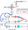 |
Fig. 1 Set-up of the FIRST-18 instrument. The injection part of the set-up, up to the fiber bundle, is basically unchanged compared to the previous version of the instrument. The recombination part on the other hand has been duplicated. The EMCCD dedicated to the measurement of the transmitted flux during the optimization procedure has also been depicted. The mirrors drawn as gray lines (just after the V-grooves and microlens arrays) are removable from the light path. Inset a) illustrates the resulting beam shapes after the anamorphic system. Inset b) is a side view of the recombination of the beams (only three beams out of nine are represented). SM: Segmented mirror. PBS: Polarizing beam splitter. μL: Microlens array. FB: Fiber bundle. VG: V-groove. P: Dispersing prism. |
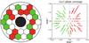 |
Fig. 2 Fiber configurations of the entrance pupil, the green and red colors corresponding to each of the two sets of nine fibers. The corresponding polychromatic (u, v) plane coverage is represented in the right panel. For clarity, the (u, v) plane coverage of each nine-fiber configuration is not symmetrized. |
After the first light of the instrument obtained in 2010 (Huby et al. 2012), efforts have been focused on improving the stability, sensitivity, and dynamic range achievable with FIRST. The injection part of the instrument (including the pupil imager, the Iris AO segmented mirror used to steer the beams precisely on the fiber cores that are gathered in the fiber bundle, from Fiberguide Industries) is basically unchanged; however, significant upgrades have been carried out in the recombination part of the instrument, as can be seen in Fig. 1.
Assuming that the noise is uncorrelated between the baselines – a reasonable assumption in the photon-noise-limited regime – the dynamic range increases with the number of visibility and closure phase measurements (Baldwin & Haniff 2002; Lacour et al. 2011; Le Bouquin & Absil 2012). The main development was therefore aimed at increasing the number of subpupils, leading to the FIRST-18 instrument, in reference to the two sets of nine subpupils that are recombined. The non-redundancy of the linear recombination configuration is a technical limit: standard V-groove chips offer 48 spaces where fibers can be positioned. The most compact nine-fiber configuration requires nmax = 44 spaces, while the 10-fiber and 11-fiber ones require 55 and 75 spaces, respectively. In addition, the nine-fiber configuration is also a compromise between the available space on the bench (defining the focal length f′ of the imaging lens), the diffraction pattern width (f′λ/D, where D is the V-groove pitch and also the collimated beam size at the fiber output) and the sampling of the highest frequency fringe pattern (of period  ) that fits the detector dimensions. For these reasons, two sets of nine fibers are recombined independently. Given the 30 available subpupils in the obstructed telescope pupil (see Fig. 2), our selected fiber configuration using 18 of them gives access to 73% of all possible independent baselines. Since the instrument is mounted at the Cassegrain focus of the telescope, the (u, v) plane coverage does not rotate during the night and is stable in time. However, the (u, v) plane coverage is significantly extended thanks to the broad wavelength range, as illustrated in Fig. 2.
Each recombination scheme of the beams is built on the same design as for the previous version. The collimated beams coming from the V-grooves are reshaped thanks to anamorphic systems that mimic the slit of a spectrometer consisting of dispersing prisms (see Fig. 1). The anamorphic system has been designed to satisfy the Nyquist-Shannon sampling condition for the highest frequency fringe pattern (for a given focal length of the imaging lens), on the one hand, and to reach a high spectral resolution, on the other. This is achieved thanks to a four-lens (2 spherical and 2 cylindrical lenses) afocal system performing a beam elongation of 20 in the direction of dispersion and a compression of 7 in the orthogonal direction. The two fringe patterns are imaged on the same detector side by side along the wavelength axis. Spectral filters have been inserted in each arm in order to avoid overlapping of the patterns. In the center of the detector, the fringe patterns are cut at 600 nm and 850 nm, thereby defining the spectral range of the instrument.
Improvement of the data quality has also been provided by the use of a more efficient detector, Hamamatsu EMCCD camera with maximal EM gain of 1200, quantum efficiency of 90%, 77% and 54% at 600, 700, and 800 nm, respectively, and 512 × 512 pixels 16 μm wide. The overall mechanical stability has been enhanced, too, allowing objects to be observed up to 40° from zenith without significant loss of flux due to mechanical flexures.
2.2. Acquisition procedure
Observation log.
Capella was observed in October 2011, July 2012, and December 2012 with FIRST-18 mounted on the 3 m Shane telescope at Lick Observatory. The observation log is reported in Table 1. Several bright (0 ≲ R ≲ 3) single stars were observed immediately before/after Capella, so they serve as calibrator for closure phase measurements and baseline calibration (see Sect. 3.2).
The acquisition procedure is similar to the description given in Huby et al. (2012). One data set comprises fringe sequences, fiber calibration files (every fiber diffraction pattern is recorded individually), and background files. However, this procedure has been significantly shortened compared to the previous observations thanks to implementing a dedicated optimization path in the optical set-up. The injection of the flux into the fibers is indeed very sensitive and must be optimized at every target switch, to compensate for residual mechanical flexures occurring in the instrument but also in the AO system. While this optimization was done one fiber at a time in 2010 (by scanning the corresponding micro-segment and measuring the transmitted flux directly on the science camera), it is now done simultaneously for all fibers thanks to a motorized mirror system that allows imaging all the output fibers on a dedicated detector. The 18 corresponding micro-segments can therefore be scanned at the same time. The optimization is now completed in less than two minutes leading to a substantial gain in time and stability.
2.3. Data reduction
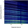 |
Fig. 3 Mean power spectral density computed from 5000 50 ms-images for Capella on 2011 Oct. 16 using data from a single V-groove. The color-scale has been adjusted by discarding the zero-frequency peak (not visible in the image). The fitted peak positions are superposed as dashed white lines only on the left part of the image for better visibility. The (telluric) absorption line appearing at spectral channel number 147 is exactly vertical, showing that the distortion in the image has been effectively corrected. At least 27 different peaks are clearly visible out of the 36 expected ones. |
The basic principles of the FIRST data analysis are based on the P2VM method (Pixel to Visibility Matrix), which was first developed for the AMBER instrument at the VLTI (Millour et al. 2004) and subsequently adapted to FIRST data, as described in more detail in Huby et al. (2012). The current data reduction process consists of the following steps:
-
background (including dark current) subtraction;
-
optical distortion correction;
-
spectral calibration based on the fitting of telluric absorption lines and features of the stellar spectrum;
-
fitting of the fringe spatial frequencies by adjusting the peak positions in the mean power spectral density;
-
calibration of the P2VM matrix from individual fiber profiles and spatial frequencies;
-
pseudo-inversion of the P2VM matrix and computation of the best parameter sets in the least-squares sense;
-
closure phase computation;
-
closure phase calibration by measurements obtained on an unresolved target.
The distortion mentioned in the second step of the reduction results from astigmatism introduced by the prism and has an amplitude of about 10−15 pixels. The shape of this distortion is evaluated by detecting the position of the deepest telluric absorption line and is corrected by horizontally interpolating and shifting the image values.
The spectral calibration is done using the UVES sky emission atlas Hanuschik (2003). Because the light is spectrally dispersed through an SF2-prism, there are two parameters that define the wavelength as a function of the pixel: the angle of incidence on the prism i, which affects the spectral resolution, and the central wavelength λ0. The continuum of the spectrum is fitted and subtracted, leaving only (stellar and telluric) absorption features. The same procedure is applied to the synthetic spectrum, and the parameters i and λ0 are retrieved by maximizing the correlation product between the two spectra. A fine adjustment is then performed by fitting the peak positions of the power spectral density computed over all images. The results of this fit are shown in Fig. 3 where the fitted peak positions are superposed on the mean power spectral density.
After applying the P2VM method, the complex coherent fluxes are thus retrieved and their phases combined to estimate closure phases. The data reduction output comprises 84 closure phase measurements for each of about 180 spectral channels from 600 nm to 850 nm. Since spatial frequency depends on wavelength, a specific signal appears in the closure phase plotted as a function of wavelength, depending on the structure of the target.
 |
Fig. 4 Closure phase measurements obtained on 19 October 2011 (black points with rescaled error bars such that the reduced χ2 per spectral channel is unity) and best fit model (red points) computed from the best estimates of the binary parameters. |
2.4. Fitting of a binary model
The final step in the analysis consists of fitting the closure phase estimates with a binary model. Three parameters are optimized by minimizing the χ2 function: two angular parameters defining the position of the companion, α and δ, and a flux ratio for each spectral channel, ρ(λ). The closure phase model function corresponding to a binary directly reads as (Le Bouquin & Absil 2012) 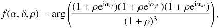 (1)with
 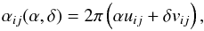 (2)where uij and vij are the projections of the spatial frequency vector sij corresponding to the subpupils i and j, on two orthonormal axes defined by the segmented mirror reference frame (see Sect. 3.2 for details concerning the baseline calibration). This vector expresses as sij = Bij/λ with Bij the baseline vector represented in the telescope pupil.
The χ2 function is therefore three dimensional. For every spectral channel, the contributions of all nCP closure phases are added quadratically: 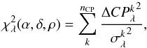 (3)with
  the error on closure phase k at wavelength λ and
  (4)is the phase difference between the data and the model, defined modulo 2π.
Under the assumption that the noise affecting the data follows a Gaussian distribution, the likelihood function can be derived from the χ2 function by  (5)The proportional symbol is a reminder that the likelihood function is normalized afterwards.
The optimal value for a given parameter can then be retrieved after marginalizing the likelihood function, i.e. by integrating over all other parameters. For the α parameter for instance, it is expressed as  Similarly, a circular permutation over the set of parameters leads to ℒλ(δ) and ℒλ(ρ). For each spectral channel, the optimal parameter sets
  are then determined by the median value of these probability densities, and the associated error bars are defined as the 68% confidence interval.
The λ dependence has been noted differently for the position parameters and the flux ratio since the position of the companion is achromatic. The  and
and  have therefore been averaged in order to determine the final position
  . Around 20% of the data points with the worst error bars have not been taken into account in computing the averaged position, in order to discard aberrant points. The associated error bars on
  and
and  are computed from the standard deviation of the respective distributions.
3. Results
3.1. The case of Capella
The calibrated closure phases of Capella are shown in Fig. 4. As is readily apparent, large deviations from the null closure phase are detected. Large phase changes of ~± π indeed occur when the observed object is centrosymmetric, indicating here that the flux ratio between the two components is close to unity, as is expected for the Capella binary system at visible wavelengths. That the transitions are smooth indicates that the flux ratio is not exactly equal to one. Thus these observations have clearly resolved the binary system.
Companion position measurements for the outer Algol system (C relative to A+B) converted into angular separation and position angle.
However, some of these phase transitions occur in the opposite direction than expected by the best fit model (see the second closure phase graph in the first row of Fig. 4 for instance). This effect is observed in around 6% of all closure phase measurements (84 × 2 closure phases per date of observation). A possible explanation is that the measurements may be affected by an uncalibrated bias on the imaginary part of the bispectrum. In this case, a sharp transition from 0 to ± π (imaginary part initially equal to 0) can therefore be turned into a smoother transition from 0 to π or −π, depending on the sign of the bias offset.
This is most likely the reason the minimum of the reduced χ2 function is generally much larger than 1. It reaches up to ~40 (for one spectral channel) in the worst cases. Therefore, prior to computing the likelihood functions, the statistical error bars are scaled such that the minimum of the reduced χ2 function per spectral channel is 1 (error bars in Fig. 4 are rescaled accordingly).
Another consequence of these transitions in the wrong direction is that it sharpens the transition when averaging closure phase datasets. The mean value of two transitions in the opposite directions will indeed result in values globally closer to ±180° or 0°. This can potentially translate into flux ratios that are biased toward unity. As detailed in the next section, this eventuality cannot be completely discarded when analyzing the spectral flux ratio.
It can be noted, though, that averaging over the closure phase was performed using complex phasors in order to take into account that the phase can only be measured modulo 2π. This is needed to compute the correct phase, especially in the case of phases around ± 180°, but that obviously does not prevent such a bias effect. However, the final flux ratio estimates are assumed to be less affected by this bias, since they result from the average of two independent measurements provided by the two sets of simultaneously recombined fibers, and also from the average of the different dates of observations.
Since the source of this bias is still unknown (photon bias only affects the real part of the bispectrum as established by Wirnitzer 1985), this effect only becomes obvious once the best fit model has been determined. There is thus no objective criterion that could allow distinguishing these biased data a priori. Nonetheless, closure phase error bars resulting from the average over all datasets corresponding to one date of observation are necessary larger when there is an uncertainty on the transition direction. As can be seen in Fig. 4, error bars are much larger around phase transitions. As a consequence, these points are less weighted in the fit.
Angular parameter estimates for Capella at different observation dates.
3.2. Orbit
The analysis of our results concerning the companion position requires calibrating the (u,v) plane, that is, a calibration of the baseline lengths and orientations (as explained by Woillez & Lacour 2013, under the imaging baseline section). For the fit, the baselines are conveniently defined by their theoretical lengths and orientation taken in a reference frame linked to the segmented mirror. However, to be scientifically useful, these need to be transformed into the angular separation of the binary and its position angle relative to north. Two aspects have to be considered for the calibration:
-
the magnification factor between the telescope pupil and the pupilthat is imaged in the FIRST instrument can vary with thealignment;
-
the rotation angle between the sky east-west / north-south orientation and the reference frame linked to the segmented mirror orientation.
The rotation of the pupil plane is caused by the periscope sending the beam from the adaptive optics bench towards the hole through the FIRST bench. It uses a mirror combination working at angles different from 45° that therefore induces an unknown rotation of the pupil relative to the subpupils.
The calibration over all baselines can thus be performed by estimating two parameters: a scaling factor and a rotation angle. This is done by measuring the position of another well-known binary star, using the same data reduction pipeline as for Capella. Among the binary systems observed at the same epochs as Capella, the triple system of Algol (δ Per) is an ideal calibrator. The inner system (Algol A of type B8V and Algol B of type K2IV) of orbital period 2.87 days and semi-major axis of 2.3 mas is unresolved by a 3 m telescope. On the other hand, the outer system (Algol A+B and Algol C of type F1V) of orbital period ≈680 days, semi-major axis of 93.8 mas, and flux ratio estimated to 10 at visible wavelengths is detected well by FIRST-18. Its orbital period is much longer than the Capella period (104 days), and this makes it a suitable target for the baseline calibration.
The relative positions of Algol A+B and C have therefore been estimated for several dates during the various runs, as shown in Table 1. The results are shown in Table 2. The position parameters have been converted into polar coordinates in order to derive the angle for the rotation to be applied to the field of view. The predicted positions are computed from the orbit resulting from the measurements with the CHARA interferometer fitted by Baron et al. (2012).
The Algol system was observed twice during both the October 2011 and December 2012 observing runs. In both cases, multiple observations of the systems within a given observing run yield consistent calibration factors at the 2σ level or better (see Table 2). This confirms the expectation that the rotation of the pupil in comparison with the FIRST subpupils is stable over the duration of an observing run since the injection part of the set-up was not modified during the course of each run. In October 2011, uncertainties on the calibration factors are much greater on October 16 than on October 19, probably as a consequence of changes in r0 (see Table 1) and short atmospheric coherence time. While the latter could not be measured, the shorter integration times used on October 16, which results from a compromise between sensitivity and fringe visibility, is indicative of a shorter timescale for atmospheric turbulence. We therefore used the estimated position of Algol C regarding Algol A+B on October 19 to correct for the pupil rotation and scaling factor for all three dates of observation in October 2011. For the December 2012 observing run, we used the weighted average of both observations of Algol since they are similar in precision.
The final relative astrometry of the Capella system throughout our observations is shown in Fig. 5. The orbit computed from the model parameters fitted by Torres et al. (2009) is drawn for comparison. Table 3 presents both uncorrected and corrected (field rotation and scaling factor taken into account) estimates, along with their associated uncertainties. Most estimates agree with the predicted positions within the 1-σ range. However, the positions measured in 2011 seem to be affected by a small systematic error of about 2 mas along the north-south direction (see Fig. 5, bottom). It is plausible that this results from the baseline calibration, since all three points have been calibrated by the same astrometric estimate for the Algol system. Ideally, the calibrator should have been observed with sufficient accuracy on the three different dates.
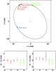 |
Fig. 5 Capella companion positions relative to the predicted orbit. Top: measured positions at different epochs: red for October 2011, blue for July 2012, and green for December 2012. Expected companion positions are marked as black dots and measurement points with error bars. Bottom: difference between the estimated and expected values of the projection of the binary separation along the right ascension and declination axes. Each point corresponds to one observation date arranged in chronological order: 2011 October 16, 17 and 19, 2012 July 29 and 2012 December 19 and 20. |
3.3. Spectral model
FIRST measurement of the flux ratio per spectral channel.
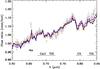 |
Fig. 6 Flux ratio for the Capella binary as a function of wavelength as measured with FIRST (gray diamonds). All curves represent predicted flux ratio spectra based on the PHOENIX grid of models and the set of solar abundances from Asplund et al. (2009). The blue dot-dashed curve shows the predicted flux ratio spectrum for the stellar parameters inferred by Torres et al. (2009), while the solid black curve represents the formal best fit (in the χ2 sense) to the flux ratio spectrum from the solar metallicity model grid. The red dashed curve shows the best fit for the model grid for a metallicity of [m/H] = + 0.5. Stellar parameters for all three models are listed in Table 5. The main atomic and molecular features that drive the model fitting are identified. |
Along with the astrometry of the binary, our analysis also yields a “spectrum” of the binary flux ratio, ρ(λ). We inspected the quality of the flux ratio spectra from each individual night and for each of the two separate V-grooves. As expected given seeing conditions, the flux ratios measured on December 2012 are of much worse quality than those from October 2011. Similarly, the July 2012 flux ratio spectrum is very noisy, owing to observations taken during early morning twilight. While the astrometric position estimates from these epochs benefit from the average of all spectral channels and are thus reasonably accurate, the flux ratio spectra obtained during the 2012 runs have been discarded for the spectral analysis. We therefore averaged all October 2011 datasets to produce a final flux ratio spectrum for the Capella binary system. The resulting final spectral resolution is about 1.5 pixel as determined from data taken using a monochromatic laser beam. Uncertainties on the flux ratio spectrum were estimated as the standard deviation of the mean over the datasets. These results are available in Table 4.
The flux ratio spectrum obtained with FIRST agrees with historical measurements of the binary taken within our wavelength range at the ≲2σ level. Furthermore, our spectrally dispersed observations reveal an overall slope that is consistent with data over a broader range and confirm that the cool component of the system is increasingly brighter at longer visible wavelengths. We find that the flux ratio reversal occurs at a wavelength of 0.64 ± 0.01 μm. In addition to its general slope, the FIRST flux ratio spectrum reveals finer structures, such as a sharp peak at 0.655 μm and two broad dips around 0.69−0.75 μm and 0.78−0.84 μm. Both can be traced to the difference in effective temperature between the two stars, which leads to photospheric features of different depths: the first is Hα (the slight mismatch in wavelength results from a mild inaccuracy in our wavelength solution) while the last two are molecular bands (most notably TiO and CN) that are characteristic of cool photospheres. These spectral features are a direct confirmation that the infrared-bright component is cooler than the visible-bright one.
To quantify the constraint on stellar properties provided by the FIRST flux ratio spectrum, we use the most recent BT-Settl models1 partially published in a review by (Allard et al. 2012a) and described by Allard et al. (2012b). These model atmospheres are computed with the PHOENIX multipurpose atmosphere code version 15.5 (Allard et al. 2001) solving the radiative transfer in 1D spherical symmetry, with the classical assumptions: hydrostatic equilibrium, convection using the mixing length theory, chemical equilibrium, and a sampling treatment of the opacities. The models use a mixing length as derived by the radiation hydrodynamic simulations of Ludwig et al. (2002, 2006) and Freytag et al. (2010, 2012) and a radius as determined by the Baraffe et al. (1998) interior models as a function of the atmospheric parameters (Teff, log g, [m/H]). The reference solar elemental abundances used in this version of the BT-Settl models are those defined by Asplund et al. (2009). For solar metallicity and higher, no α element enhancement is required.
The PHOENIX library includes stellar spectra with a 100 K and 0.5 sampling in Teff and log g, respectively. We explored the parameter space as follows: each model consisted of two pairs of stellar parameters (Teff and log g for each component). The model flux ratio was computed using the same sampling and resolution as the FIRST data and normalized so as to match the observed median flux ratio. Since the PHOENIX emission spectra are given per unit surface area, this normalization is equivalent to setting the ratio of stellar radii to match the median flux ratio best in our spectral bandpass. In principle, our analysis could consider this ratio as a free parameter in the fit instead. However, since the FIRST flux ratios are in good agreement with previous flux ratio estimates of the binary, we do not expect to gain additional insight into the ratio of stellar radii. We therefore decided to remove one free parameter from our fit by using this a priori normalization to ensure that the model fitting was primarily attempting to reproduce the global slope and finer spectral features, which only depend on the stellar effective temperatures and surface gravities. We believe that our data are more apt to constrain the latter. Nonetheless, we note that our normalization for the best fit models is consistent at the 1σ level with the stellar radii ratio of 0.737 ± 0.044 estimated by Torres et al. (2009).
We have thus created a grid of flux ratio spectra that depends on four parameters, the effective temperature and surface gravity of both components, while approximately maintaining the average stellar luminosity ratio in the FIRST bandpass. By performing a wide grid search around the stellar parameters derived by Torres et al. (2009), the best fitting model has the following parameters:  K,
K,  K, and log ghot = log gcool = 2.0. This combination of stellar parameters yields a reasonably good match to the observed flux ratio spectrum (reduced χ2 = 2.89, see Fig. 6 and Table 5). We note that there is another peak appearing in the likelihood distribution, which corresponds to a model with
  K,
K,  K and leads to a marginally poorer χ2, providing a sense for the uncertainties on the derived stellar effective temperatures.
The stellar parameters derived here are significantly different from those estimated by Torres et al. (2009), although the effective temperatures are only 4−7% lower than their nominal values. As shown in Fig. 6, the higher effective temperatures proposed by Torres et al. (2009) also result in detectable molecular features in the flux ratio spectrum, although they are less marked than in our data (especially for the 0.78−0.84 μm feature). This issue can be partially alleviated by using synthetic stellar spectra that correspond to lower surface gravity strengths. However, the overall quality of the fit is much poorer (see Table 5).
Stellar parameters of the PHOENIX atmospheric models used in this analysis from Allard et al. (2012b) assuming the set of solar abundances from Asplund et al. (2009).
One solution for improving the fit consists in assuming a metal-rich composition. Using the series of PHOENIX models computed for [m/H] = + 0.5 (where elemental abundances are increased uniformly from the set of solar abundances), we find that the FIRST data are best fit with effective temperatures of 5600 and 4900 K and surface gravities of log ghot = 2.5 and log ghot = 2.5. This model is significantly better (reduced χ2 = 2.31, see Fig. 6) than the best fit model at solar metallicity, and it has stellar properties in good agreement with Torres et al. (2009). However, the super-solar metallicity is at odds with all estimates for the components of the system. We thus conclude that the observed flux ratio spectrum of the Capella binary does not conform perfectly to the prediction of stellar atmosphere models.
Breaking down the information provided by the FIRST flux ratio spectrum, it appears that the overall slope across the 0.6−0.85 μm is reasonably well fit with both the nominal effective temperatures and the lower values preferred by the model fitting above, so long as the difference in effective temperatures between the two components is about 10−12%. Thus it appears that the spectral features, specifically the depth of the molecular bands, represent the main culprit in forcing the fit away from the nominal stellar parameters. As mentioned in the previous section, we cannot exclude with certainty that a subtle bias in our data analysis is affecting the resulting flux ratio spectrum, possibly because the system is close to a flux ratio of one. However, we find it extremely unlikely that this bias could affect the wavelengths where molecular features are present, but not the adjacent continuum. Indeed, such biases are expected to be present where the closure phases undergo a large shift (from ± π to 0 for instance), as explained in Sect. 3.1. This is therefore expected to be independent of spectral features, since the occurrence of these shifts only depends on the spatial frequencies (∝B/λ, B corresponding to the baseline) involved in the closure triangle. We thus believe that the mismatch between observations and models is instead an astrophysical effect.
Cooler effective temperatures, lower surface gravities, and/or higher metallicity are all factors that result in deeper molecular bands in each component and in an increased difference in their strength, in turn resulting in deeper features in the flux ratio spectrum as well. Since the stellar parameters of the Capella binary have been precisely determined, our FIRST flux ratio spectrum thus demonstrates that the molecular absorption bands in the spectra of each component are deeper than predicted by the models. One possible explanation for this shortcoming of the models is that the molecular opacities are underestimated in the models, because of incomplete line lists being used and/or underestimated oscillator strengths. Departures from local thermal equilibrium in stellar atmospheres can induce substantial effects for A-type stars but are negligible in the range of effective temperatures relevant to the Capella system. The two molecules that account for most of the opacity in the spectral features observed with FIRST are TiO and CN. For the former molecule, the version of the PHOENIX models used here are based on the line lists and oscillator strengths from Plez (1998). The CN line list and oscillator strengths were adopted from the SCAN database (Jorgensen & Larsson 1990). The TiO molecule, whose features are frequent in a broad range of cool stars, is much better calibrated, so we conclude that the reason for the underprediction of these features by current atmospheric features most likely stems from the treatment of the CN molecule, either through the incompleteness of its line list or as a result of oscillator strengths that are too low.
4. Summary of findings and conclusion
To demonstrate the capabilities of a fibered aperture masking instrument like FIRST to provide valuable spectrally-dispersed information on binary systems whose separation is close to the diffraction limit, the results presented in this paper focused on the binary star Capella. Its separation is indeed comparable to the diffraction limit and its flux ratio close to unity at visible wavelengths. Capella was observed at three different epochs between 2011 and 2012 with FIRST-18 mounted on the 3 m Shane telescope of Lick Observatory (using its adaptive optics system as a fringe tracker). The secondary component was detected at or slightly below the diffraction limit of the telescope at visible wavelengths with an accuracy well below a tenth of the diffraction limit. This first achievement illustrates the high angular resolution capability of the instrument.
Using FIRST, we also directly measured, for the first time, the flux ratio of the binary system at a spectral resolution of R ~ 300 between 600 and 850 nm. This spectral range gives access to spectral features (Hα line, TiO, and CN bands) that are quite influential when comparing the observed flux ratio spectrum with predictions based on the PHOENIX library of synthetic spectra. The effective temperatures derived from this analysis are slightly offset (by 5−7%) from those estimated by Torres et al. (2009) based on the extensive literature on this system. While we cannot exclude a subtle bias affecting our flux ratio measurements arising from the fact that the flux ratio is close to unity, this discrepancy probably indicates that the photospheric models used to predict the synthetic spectra are based on incomplete line lists and/or underestimated oscillator strengths for molecules commonly found in G- and K-type giants (most likely CN). This conclusion illustrates the power of FIRST to provide valuable spectral information to characterize binary systems.
Acknowledgments
The authors would like to thank the staff at the Lick Observatory who provided an efficient and friendly support, especially for mounting the FIRST instrument and during the observing nights: Keith Baker, Bob Owen, Erik Kovacs, Kostas Chloros, Donnie Redel, Wayne Earthman, Paul Lynam and Pavl Zachary. They are also grateful to Dr. Bolte, Director of the University of California Observatories, for his commitment to the project and generous telescope time allocation. They also thank the students from U.C. Berkeley who helped during the observing runs, S. Goeble and K. J. Burns, or helped improve the data reduction software, B. Bordwell. Dr. Helmbrecht, the President and Founder of Iris AO, is also deeply thanked for his precious support concerning the segmented mirror. E. Huby would like to thank Alain Delboulbé for his valuable experience and recommendation concerning the optical bench dedicated to equalizing the fiber lengths. Finally, we acknowledge financial support from the Programme National de Physique Stellaire (PNPS) of the CNRS/INSU, France, and from a Small Research Grant of the American Astronomical Society. F. Marchis’s contribution to this work was supported by NASA Grant NNX11AD62G and by the National Science Foundation under Award Number AAG-0807468.
References
- Allard, F., Hauschildt, P. H., Alexander, D. R., Tamanai, A., & Schweitzer, A. 2001, ApJ, 556, 357 [NASA ADS] [CrossRef] [Google Scholar]
- Allard, F., Homeier, D., & Freytag, B. 2012a, Roy. Soc. London Philos. Trans. Ser. A, 370, 2765 [Google Scholar]
- Allard, F., Homeier, D., Freytag, B., & Sharp, C. M. 2012b, in EAS Publ. Ser. 57, eds. C. Reylé, C. Charbonnel, & M. Schultheis, 3 [Google Scholar]
- Anderson, J. A. 1920, ApJ, 51, 263 [NASA ADS] [CrossRef] [Google Scholar]
- Asplund, M., Grevesse, N., Sauval, A. J., & Scott, P. 2009, ARA&A, 47, 481 [NASA ADS] [CrossRef] [Google Scholar]
- Baldwin, J. E., & Haniff, C. A. 2002, Phil. Trans. R. Soc. London, Ser. A, 360, 969 [Google Scholar]
- Baraffe, I., Chabrier, G., Allard, F., & Hauschildt, P. H. 1998, A&A, 337, 403 [NASA ADS] [Google Scholar]
- Barlow, D. J., Fekel, F. C., & Scarfe, C. D. 1993, PASP, 105, 476 [NASA ADS] [CrossRef] [Google Scholar]
- Baron, F., Monnier, J. D., Pedretti, E., et al. 2012, ApJ, 752, 20 [NASA ADS] [CrossRef] [Google Scholar]
- Blasius, T. D., Monnier, J. D., Tuthill, P. G., Danchi, W. C., & Anderson, M. 2012, MNRAS, 426, 2652 [NASA ADS] [CrossRef] [Google Scholar]
- Campbell, W. W. 1899, ApJ, 10, 177 [NASA ADS] [CrossRef] [Google Scholar]
- Chang, M. P., & Buscher, D. F. 1998, in SPIE Conf. Ser. 3350, ed. R. D. Reasenberg, 2 [Google Scholar]
- Cieza, L. A., Lacour, S., Schreiber, M. R., et al. 2013, ApJ, 762, L12 [NASA ADS] [CrossRef] [Google Scholar]
- Evans, T. M., Ireland, M. J., Kraus, A. L., et al. 2012, ApJ, 744, 120 [NASA ADS] [CrossRef] [Google Scholar]
- Freytag, B., Allard, F., Ludwig, H.-G., Homeier, D., & Steffen, M. 2010, A&A, 513, A19 [NASA ADS] [CrossRef] [EDP Sciences] [Google Scholar]
- Freytag, B., Steffen, M., Ludwig, H.-G., et al. 2012, J. Comput. Phys., 231, 919 [Google Scholar]
- Grady, C. A., Muto, T., Hashimoto, J., et al. 2013, ApJ, 762, 48 [NASA ADS] [CrossRef] [Google Scholar]
- Haniff, C. A., Mackay, C. D., Titterington, D. J., et al. 1987, Nature, 328, 694 [NASA ADS] [CrossRef] [Google Scholar]
- Hanuschik, R. W. 2003, A&A, 407, 1157 [NASA ADS] [CrossRef] [EDP Sciences] [Google Scholar]
- Hinkley, S., Carpenter, J. M., Ireland, M., & Kraus, A. L. 2011, ApJ, 730, L21 [NASA ADS] [CrossRef] [Google Scholar]
- Huby, E., Perrin, G., Marchis, F., et al. 2012, A&A, 541, A55 [NASA ADS] [CrossRef] [EDP Sciences] [Google Scholar]
- Hummel, C. A., Armstrong, J. T., Quirrenbach, A., et al. 1994, AJ, 107, 1859 [NASA ADS] [CrossRef] [Google Scholar]
- Jorgensen, U. G., & Larsson, M. 1990, A&A, 238, 424 [NASA ADS] [Google Scholar]
- Lacour, S., Thiébaut, E., & Perrin, G. 2007, MNRAS, 374, 832 [NASA ADS] [CrossRef] [Google Scholar]
- Lacour, S., Tuthill, P., Amico, P., et al. 2011, A&A, 532, A72 [NASA ADS] [CrossRef] [EDP Sciences] [Google Scholar]
- Lagrange, A.-M., Milli, J., Boccaletti, A., et al. 2012, A&A, 546, A38 [NASA ADS] [CrossRef] [EDP Sciences] [Google Scholar]
- Le Bouquin, J.-B., & Absil, O. 2012, A&A, 541, A89 [NASA ADS] [CrossRef] [EDP Sciences] [Google Scholar]
- Ludwig, H.-G., Allard, F., & Hauschildt, P. H. 2002, A&A, 395, 99 [NASA ADS] [CrossRef] [EDP Sciences] [Google Scholar]
- Ludwig, H.-G., Allard, F., & Hauschildt, P. H. 2006, A&A, 459, 599 [NASA ADS] [CrossRef] [EDP Sciences] [Google Scholar]
- Merrill, P. W. 1922, ApJ, 56, 40 [NASA ADS] [CrossRef] [Google Scholar]
- Millour, F., Tatulli, E., Chelli, A. E., et al. 2004, in SPIE Conf. Ser. 5491, ed. W. A. Traub, 1222 [Google Scholar]
- Newall, H. F. 1899, MNRAS, 60, 2 [NASA ADS] [Google Scholar]
- Perrin, G., Lacour, S., Woillez, J., & Thiébaut, E. 2006, MNRAS, 373, 747 [NASA ADS] [CrossRef] [Google Scholar]
- Plez, B. 1998, A&A, 337, 495 [NASA ADS] [Google Scholar]
- Sanchez-Bermudez, J., Schödel, R., Alberdi, A., & Pott, J. U. 2012, J. Phys. Conf. Ser., 372, 012025 [NASA ADS] [CrossRef] [Google Scholar]
- Torres, G., Claret, A., & Young, P. A. 2009, ApJ, 700, 1349 [NASA ADS] [CrossRef] [Google Scholar]
- Weber, M., & Strassmeier, K. G. 2011, A&A, 531, A89 [NASA ADS] [CrossRef] [EDP Sciences] [Google Scholar]
- Wirnitzer, B. 1985, J. Opt. Soc. Am. A, 2, 14 [NASA ADS] [CrossRef] [Google Scholar]
- Woillez, J., & Lacour, S. 2013, ApJ, 764, 109 [NASA ADS] [CrossRef] [Google Scholar]
All Tables
Companion position measurements for the outer Algol system (C relative to A+B) converted into angular separation and position angle.
Stellar parameters of the PHOENIX atmospheric models used in this analysis from Allard et al. (2012b) assuming the set of solar abundances from Asplund et al. (2009).
All Figures
|
Fig. 1 Set-up of the FIRST-18 instrument. The injection part of the set-up, up to the fiber bundle, is basically unchanged compared to the previous version of the instrument. The recombination part on the other hand has been duplicated. The EMCCD dedicated to the measurement of the transmitted flux during the optimization procedure has also been depicted. The mirrors drawn as gray lines (just after the V-grooves and microlens arrays) are removable from the light path. Inset a) illustrates the resulting beam shapes after the anamorphic system. Inset b) is a side view of the recombination of the beams (only three beams out of nine are represented). SM: Segmented mirror. PBS: Polarizing beam splitter. μL: Microlens array. FB: Fiber bundle. VG: V-groove. P: Dispersing prism. |
| In the text | |
|
Fig. 2 Fiber configurations of the entrance pupil, the green and red colors corresponding to each of the two sets of nine fibers. The corresponding polychromatic (u, v) plane coverage is represented in the right panel. For clarity, the (u, v) plane coverage of each nine-fiber configuration is not symmetrized. |
| In the text | |
|
Fig. 3 Mean power spectral density computed from 5000 50 ms-images for Capella on 2011 Oct. 16 using data from a single V-groove. The color-scale has been adjusted by discarding the zero-frequency peak (not visible in the image). The fitted peak positions are superposed as dashed white lines only on the left part of the image for better visibility. The (telluric) absorption line appearing at spectral channel number 147 is exactly vertical, showing that the distortion in the image has been effectively corrected. At least 27 different peaks are clearly visible out of the 36 expected ones. |
| In the text | |
|
Fig. 4 Closure phase measurements obtained on 19 October 2011 (black points with rescaled error bars such that the reduced χ2 per spectral channel is unity) and best fit model (red points) computed from the best estimates of the binary parameters. |
| In the text | |
|
Fig. 5 Capella companion positions relative to the predicted orbit. Top: measured positions at different epochs: red for October 2011, blue for July 2012, and green for December 2012. Expected companion positions are marked as black dots and measurement points with error bars. Bottom: difference between the estimated and expected values of the projection of the binary separation along the right ascension and declination axes. Each point corresponds to one observation date arranged in chronological order: 2011 October 16, 17 and 19, 2012 July 29 and 2012 December 19 and 20. |
| In the text | |
|
Fig. 6 Flux ratio for the Capella binary as a function of wavelength as measured with FIRST (gray diamonds). All curves represent predicted flux ratio spectra based on the PHOENIX grid of models and the set of solar abundances from Asplund et al. (2009). The blue dot-dashed curve shows the predicted flux ratio spectrum for the stellar parameters inferred by Torres et al. (2009), while the solid black curve represents the formal best fit (in the χ2 sense) to the flux ratio spectrum from the solar metallicity model grid. The red dashed curve shows the best fit for the model grid for a metallicity of [m/H] = + 0.5. Stellar parameters for all three models are listed in Table 5. The main atomic and molecular features that drive the model fitting are identified. |
| In the text | |
Current usage metrics show cumulative count of Article Views (full-text article views including HTML views, PDF and ePub downloads, according to the available data) and Abstracts Views on Vision4Press platform.
Data correspond to usage on the plateform after 2015. The current usage metrics is available 48-96 hours after online publication and is updated daily on week days.
Initial download of the metrics may take a while.