| Issue |
A&A
Volume 560, December 2013
|
|
|---|---|---|
| Article Number | A28 | |
| Number of page(s) | 9 | |
| Section | Extragalactic astronomy | |
| DOI | https://doi.org/10.1051/0004-6361/201321424 | |
| Published online | 02 December 2013 | |
Black-hole mass estimates for a homogeneous sample of bright flat-spectrum radio quasars
1
SISSA, via Bonomea 265,
34136
Trieste,
Italy
e-mail:
castigna@sissa.it
2
DiSAT, Università dell’Insubria, via Valleggio 11, 22100
Como,
Italy
3
INFN, Sezione di Milano Bicocca, Piazza Della Scienza 3,
20126
Milano,
Italy
4
Dipartimento di Fisica, Università “Tor Vergata”,
via della Ricerca Scientifica 1,
00133
Roma,
Italy
5
INAF-Osservatorio Astronomico di Padova, Vicolo dell’Osservatorio
5, 35122
Padova,
Italy
Received:
6
March
2013
Accepted:
16
September
2013
We have selected a complete sample of flat-spectrum radio quasars (FSRQs) from the WMAP 7 yr catalog within the SDSS area, all with measured redshift, and compared the black-hole mass estimates based on fitting a standard accretion disk model to the “blue bump” with those obtained from the commonly used single-epoch virial method. The sample comprises 79 objects with a flux density limit of 1 Jy at 23 GHz, 54 of which (68%) have a clearly detected “blue bump”. Thirty-four of those 54 have, in the literature, black-hole mass estimates obtained with the virial method. The mass estimates obtained from the two methods are well correlated. If the calibration factor of the virial relation is set to f = 4.5, well within the range of recent estimates, the mean logarithmic ratio of the two mass estimates is equal to zero with a dispersion close to the estimated uncertainty of the virial method. That the two independent methods agree so closely in spite of the potentially large uncertainties associated with each lends strong support to both of them. The distribution of black-hole masses for the 54 FSRQs in our sample with a well-detected blue bump has a median value of 7.4 × 10⁸ M⊙. It declines at the low-mass end, consistent with other indications that radio-loud AGNs are generally associated with the most massive black holes, although the decline may be, at least partly, due to the source selection. The distribution drops above log (M•/M⊙) = 9.4, implying that ultra-massive black holes associated with FSRQs must be rare.
Key words: black hole physics / accretion, accretion disks
© ESO, 2013
1. Introduction
Reliable mass estimates of black holes (BHs) in active galaxies are essential for
investigating the physics of accretion and emission processes in the BH environment and the
link between the BH growth and the evolution of galaxy stellar populations. However, getting
them is not easy, however. Dynamical mass estimates are only possible for nearby objects
whose parsec-scale BH sphere of influence can be resolved and are usually applicable to
quiescent galaxies. BH masses of luminous active galactic nuclei (AGNs) are most commonly
estimated using a technique known as single epoch virial method or, briefly, SE method.
Under the usual assumption that the broad-line region (BLR) is in virial equilibrium, the BH
mass is derived as  (1)where
RBLR is the BLR radius, ΔV is the velocity of
the BLR clouds (that can be inferred from the line width), f the virial
coefficient that depends on the geometry and kinematics of the BLR, and G
the gravitational constant.
(1)where
RBLR is the BLR radius, ΔV is the velocity of
the BLR clouds (that can be inferred from the line width), f the virial
coefficient that depends on the geometry and kinematics of the BLR, and G
the gravitational constant.
An effective way to estimate RBLR, known as “reverberation mapping”, exploits the delay in the response of the BLR to short-term variability of the ionizing continuum (Blandford & McKee 1982). The application of this technique has, however, been limited because it requires long-term monitoring of both the continuum and the broad emission lines. The SE method bypasses this problem by exploiting the correlation between the size of the BLR and the AGN optical/UV continuum luminosity empirically found from reverberation mapping (Koratkar & Gaskell 1991; Kaspi et al. 2005; Bentz et al. 2009) and expected from the photo-ionization model predictions (Koratkar & Gaskell 1991). The AGN continuum luminosity can thus be used as a proxy for the BLR size.
However, measurements of the AGN continuum may be affected by various systematics: contributions from broad Fe II emission and/or from the host galaxy and, in the case of blazars, contamination by synchrotron emission from the jet (Wu et al. 2004; Greene & Ho 2005). Fortunately, there are tight, almost linear correlations between the luminosity of the AGN continuum and the luminosity of emission lines such as Hα, Hβ, Mg II, and C IV (Greene & Ho 2005; Vestergaard & Peterson 2006; Shen et al. 2011). It is thus expedient to estimate the BH masses using the line luminosities and full widths at half maximum (FWHMs).
Nevertheless, the reliability and accuracy of the method and of the resulting mass estimates, M•, is still debated (Croom 2011; Assef et al. 2012). Each of its ingredients is endowed with a considerable uncertainty (Vestergaard & Peterson 2006; Park et al. 2012b). Recent estimates of the virial coefficient, f, differ by a factor ≃2. The luminosity-size relations have a significant scatter. In addition line widths and luminosities vary on short timescales while BH masses should not vary. These uncertainties are on top of those on the measurements of line widths and luminosities, which need to be corrected for emissions from outside the BLR. Park et al. (2012b) find that uncertainties in the size-luminosity relation and in the virial coefficient translate into a factor ≃3 uncertainty in M•. But, as pointed out by Shen (2013), other sources of substantial systematic errors may also be present.
An independent method of estimating M• rests upon fitting the optical/UV “bump” of AGNs (e.g. Malkan 1983; Wandel & Petrosian 1988; Laor 1990; Ghisellini et al. 2010; Calderone et al. 2013). In the the Shakura & Sunyaev (1973) accretion disk model the BH mass is a simple function of the frequency at which the disk emission peaks, which is a measure of the effective disk temperature and of the accretion rate, estimated by the disk luminosity, given the radiation efficiency and the inclination angle, i, which is the angle between the line-of-sight and the normal to the disk plane (Frank et al. 2002). However, this method had a limited application to estimating M• (Ferrarese & Ford 2005), mainly because reliable estimates of the intrinsic disk luminosity are very difficult to obtain. In fact, a) the inclination is generally unknown and the observed flux density is proportional to cosi, b) the observed UV bump is highly sensitive to obscuration by dust either in the circum-nuclear torus or in the host galaxy, and c) we need to subtract the contribution from the host galaxy that may be substantial particularly for the weaker active nuclei.
These difficulties are greatly eased in the case of flat-spectrum radio quasars (FSRQs) because a) the accretion disk is expected to be perpendicular to the jet direction, and indeed there is strong evidence that the jets of Fermi FSRQs are highly aligned (within 5°) with the line-of-sight (Ajello et al. 2012) so that cosi ≃ 1; b) the obscuration is expected to be negligible because blazar host galaxies are thought to be passive, dust free, ellipticals (e.g. Giommi et al. 2012, and references therein) and also the torus is likely perpendicular to the line-of-sight; and c) the contamination is also low because elliptical hosts are red, i.e. faint in the UV. However, the UV emission may be contaminated by the emission from the relativistic jet.
On the other hand, the BH mass estimates obtained by fitting the blue bump rely on several assumptions whose validity has not been fully proven (see Ghisellini et al. 2010, for a discussion): (i) the disk is described by a standard Shakura & Sunyaev (1973) model, i.e., the disk is optically thick and geometrically thin; (ii) the BH is non-rotating, of Schwarzschild type; (iii) the SED is a combination of black body spectra. If any of these assumptions does not hold, the mass estimates would be affected. An additional uncertainty source in our practical application is that photometry of the SED beyond the peak is not always available. When it is available, it is not simultaneous with the optical data determining the rising part of the SED and needs corrections for extinction within our own galaxy and, in the case of objects at high-z, for photoelectric absorption in the intergalactic medium.
A cross-check of the outcome of the two, independent, approaches for FSRQs is therefore important to verify the reliability of the underlying assumptions of either method, to estimate the associated uncertainties and to constrain the values of the parameters.
The plan of the paper is the following. The selection of the sample and the photometric data we have collected are presented in Sect. 2. In Sect. 3 we describe the components used to model the spectral energy distributions (SEDs) of our sources and the formalism to obtain the BH mass estimates from the “blue bump” fitting. In Sect. 4 we briefly deal with estimates exploiting the SE method, found in the literature, compare them with our estimates, and present the distribution of BH masses obtained from the “blue bump” fitting. Our main conclusions are summarized and briefly discussed in Sect. 5.
We adopt a standard flat ΛCDM cosmology with matter density Ωm = 0.27 and Hubble constant H0 = 71 km s-1 Mpc-1 (Hinshaw et al. 2009).
2. The sample
The Wilkinson Microwave Anisotropy Probe (WMAP) satellite has provided the first all-sky survey at high radio frequencies (≥23 GHz). At these frequencies blazars are the dominant radio-source population. We selected a complete blazar sample, flux-limited at 23 GHz (K band), drawn from the seven-year WMAP point source catalog (Gold et al. 2011).
The basic steps in our selection procedure are the following. We adopted a flux-density limit of SK = 1 Jy, corresponding to the WMAP completeness limit (Planck Collaboration 2011b), and cross-matched the selected sources with the most recent version of the blazar catalog BZCAT (Massaro et al. 2011)1. This search yielded 248 catalogued blazars. To check whether there are additional bona fide blazars among the other WMAP sources brighter than the adopted flux density limit, we collected data on them from the NASA/IPAC Extragalactic Database (NED)2, from the database by Trushkin (2003), and from the catalog of the Australia Telescope Compact Array (ATCA) 20 GHz survey (AT20G, Hancock et al. 2011). Sources qualify as bona fide blazars if they have i) a flat radio spectrum (Fν ∝ ν−α with α ≤ 0.5), ii) high variability, and iii) compact radio morphology. Based on these criteria we added seven sources to our blazar sample that satisfy the first two criteria. The third criterion is satisfied by three of them, whereas for the others no radio image is available in the NED. Our initial sample then consists of 255 blazars, 243 of which have redshift measurements.
Since we are interested in characterizing the optical/UV bump attributed to the accretion disk we restricted the sample to the 103 blazars within the area covered by the Eighth Data Release (DR8)3 of the Sloan Digital Sky Survey (SDSS), totalling over 14 000 square degrees of sky and providing simultaneous five-band photometry with limiting AB magnitudes at 95% completeness level u, g, r, i, z = 22.0, 22.2, 22.2, 21.3, 20.5 (Abazajian et al. 2004). With the exception of WMAP7 # 274, these objects are in the BZCAT. Moreover, since BL Lacs generally do not show the UV bump, we dropped the 19 sources classified as BL Lacs from our sample, as well as the five sources classified as blazars of uncertain type, keeping only sources classified as FSRQs. The final sample comprises 79 objects, all having spectroscopic redshift measurements.
2.1. Photometric data
For these 79 objects, we have collected, updated, and complemented the photometric data available on the NED, as described in the following.
2.1.1. SDSS DR8 data
SDSS counterparts of our FSRQs were searched by adopting their low-frequency radio coordinates which have uncertainties of ≃1 arcsec. Since the SDSS positional uncertainty adds very little to the error (the SDSS positional accuracy is of ≃0.1 arcsec) we have chosen a search radius of 3 arcsec. By construction, all our FSRQs have at least one SDSS counterpart within the search radius. In most cases we found a unique counterpart, with the SDSS photometry consistent with extrapolations from data at nearby frequencies compliant with a type-1 QSO SED plus the jet emission. Only in eight cases (WMAP7 sources with ID numbers 26, 30, 153, 182, 198, 250, 317, 353) we have found multiple counterparts; however in each case one of the sources within the search radius was much (at least 2 mag) brighter than the others and had flux densities consistent with those of the FSRQ at nearby frequencies. Thus an unambiguous SDSS counterpart was found for all our FSRQs. They have a median and an average dereddened AB r-band magnitude of 17.67 and 17.63 mag, with an rms dispersion of 1.31 mag. Thus they are generally much brighter than the 95% SDSS magnitude limit. Only one FSRQ in the sample, WMAP7 # 314, has an r-band magnitude that is slightly fainter than that limit.
We adopted the SDSS magnitudes corrected for Galactic extinction, as listed in the DR8 catalog and denoted, say, dered_g. As suggested in the DR8 tutorial4 we have decreased the DR8 u-band magnitudes by 0.04 to bring them to the AB system. The corrections to the magnitudes in the other bands are negligible. In principle, some additional extinction may take place within the host galaxy, but we expect it to be negligible because the jet sweeps out any intervening material along its trajectory. The correction for absorption in the intergalactic medium (IGM) is described in Sect. 2.1.3. For the redshift range spanned by our sources it may only be relevant in the u and g bands.
The choice of the effective wavelength corresponding to each SDSS filter depends on the convolution of the filter’s spectral-response function with the spectral shape of the source. We adopted the effective wavelengths reported in the SDSS tutorial5: 3543, 4770, 6231, 7625, and 9134 Å, for the u, g, r, i and z filters, respectively.
2.1.2. GALEX data
We looked for UV photometry for our FSRQs in the sixth data release, GR66, of the Galaxy Evolution Explorer (GALEX) satellite (Morrissey et al. 2007). GALEX provides near-UV (NUV, 1750–2800 Å) and far-UV (FUV, 1350–1750 Å) images down to a magnitude limit AB ~ 20–21 with an estimated positional uncertainty of ≃0.5 arcsec. We adopted 1535 and 2301 Å as the effective wavelengths of the FUV and NUV filters, respectively.
Again the low-frequency radio positions of FSRQs were used and a search radius of 3.5 arcsec was adopted. At least one counterpart was found for 65 objects. Multiple counterparts were found to correspond to GALEX measurements at different epochs of the same source (i.e., differences in coordinates were within the positional errors). Such multi-epoch measurements were found for 24 of our sources. In these cases we adopted their weighted average. Whenever the S/N < 3, we adopted upper limits equal to three times the error.
The UV fluxes are very sensitive to extinction within our Galaxy and, in the case of high-z objects, to photoelectric absorption in the intergalactic medium. To correct for Galactic extinction we used the values of E(B−V) given in the GR6 catalog for each source and the extinction curve by Cardelli et al. (1989), as updated by O’Donnell (1994) and normalized to A(V) = 3.1 E(B−V). The correction for absorption in the IGM is described in the next section.
2.1.3. Absorption in the intergalactic medium
Since we do not know the IGM attenuation along each line of sight we have used the effective optical depth τeff(z) = −ln [⟨ exp(−τ) ⟩], averaged over all possible lines of sight. Following Haardt & Madau (2012), we computed τeff(z) at the effective wavelengths of SDSS u and g filters (the effective optical depth in the three other SDSS filters vanishes for the redshift range of interest here) and of the two GALEX filters. The results are shown in Fig. 1 and listed in Table 1. The step-like features are due to Lyman series absorption. We have verified that adopting the spectral response of each filter instead of considering the single effective wavelengths results in a small correction in the flux densities and in the smoothing of all the edges in the optical depth as a function of redshift. Details on these calculations will be presented in a forthcoming paper (Madau & Haardt, in prep.).
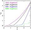 |
Fig. 1 Redshift-dependent effective optical depth for IGM absorption, averaged over all lines of sight, at the effective wavelengths of SDSS g and u bands and of the GALEX NUV and FUV bands. |
Redshift-dependent effective optical depth for IGM absorption, averaged over all lines of sight, at the effective wavelengths of the GALEX NUV and FUV bands and of SDSS the g and u bands.
2.1.4. X-ray data
We have found ROSAT data for 18 of the 79 FSRQs in our sample. However an inspection of the global SEDs indicates, for all of them, that X-ray data are clearly far from the fit of the blue bump in terms of the Shakura & Sunyaev (1973) accretion disk adopted in this paper, and more likely related to other components, such as the synchrotron or the inverse Compton ones or the emission from a bright hot X-ray corona.
2.1.5. WISE data
We have cross-correlated our FSRQs with the latest version of the Wide-field Infrared Survey Explorer (WISE; Wright et al. 2010) catalog7. Again, the coordinates of low radio-frequency counterparts were adopted and a search radius of 6.5 arcsec was chosen, consistent with WISE positional uncertainty8. We found WISE counterparts with S/N ≥ 3 in at least one band for all the 79 FSRQ in the sample. In the WISE bands where S/N < 3 we have adopted an upper limit equal to three times the error. Multiple WISE sources were found within the search radius for the FSRQs WMAP7 # 30, 126, 278, 317, and 378. In these cases we chose the brightest WISE source as the most likely counterpart. In all cases, the other sources were at least two magnitudes dimmer.
2.2. Planck data
In the Planck Early Release Compact Source Catalog (ERCSC; Planck Collaboration 2011a) we have found counterparts for 72 out of our 79 FSRQs; 47, 39, and 68 of them have ERCSC flux densities at 70, 44, and 30 GHz, respectively, and 63 have ERCSC flux densities at frequencies ≥100 GHz.
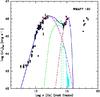 |
Fig. 2 Example of an SED fit (WMAP7 # 190). Solid blue parabola: total SED, which includes synchrotron emission, host galaxy, disk and torus emissions; dashed violet line: synchrotron from the jet; green dashed line: torus; dashed cyan line: host galaxy, taken to be a passive elliptical with MR = −23.7; dashed red line: accretion disk. Orange points: Planck data; green: WISE data; red: SDSS data; magenta: GALEX data. Black points: data taken from the NASA/IPAC Extragalactic Database (NED). At variance with what was done to compute Ld (see text), the luminosities shown here are computed assuming isotropic emission. |
3. SED modeling
Of the 79 FSRQs in our sample, 54 (i.e. 68%) show clear evidence of the optical/UV bump, interpreted as the emission from a standard optically thick, geometrically thin accretion disk model (Shakura & Sunyaev 1973). As illustrated by the example shown in Fig. 2, the global SEDs are modeled by taking several additional components into account: the Doppler-boosted synchrotron continuum modeled following Donato et al. (2001); a passive elliptical host galaxy template (see, e.g., Giommi et al. 2012); the dusty AGN torus emission based on a type-1 QSO template (BQSO1) from the Polletta et al. (2007)9 SWIRE template library.
The fit of the global SED was made using six free parameters. Four are those of the blazar sequence model for the synchrotron emission (the 5 GHz luminosity, the 5 GHz spectral index, the junction frequency between the low- and the high-frequency synchrotron template and the peak frequency of νLν, Donato et al. 2001). The remaining two parameters refer to the accretion disk model (i.e., the normalization and the peak frequency). The other components are fixed. The host galaxy template is an elliptical (Mannucci et al. 2001) with an absolute magnitude of MR = −23.7, as in Giommi et al. (2012). The normalization of the torus template was computed from that of the accretion disk emission, requiring that the torus/accretion disk luminosity ratio is equal to that of the Polletta et al. (2007) BQSO1 template.
We stress that accurate fits of the global SEDs are beyond the scope of the present paper whose main purpose is to estimate the BH masses by fitting the optical/UV bump with a Shakura & Sunyaev (1973) model, as discussed, below. The consideration of the other components, fitted taking all the data we have collected into account, is mainly relevant to checking whether they may contaminate the emission from the accretion disk. In many cases, the lack of simultaneity of the measurements does not allow reliable fits of the other components. Still for the 54 objects with clear evidence of the blue bump, the data were enough either to estimate the amount of contamination or to signal points that should be better taken as upper limits to the blue bump emission.
The thermal emission from the accretion disk is modeled as a combination of black bodies
with temperatures depending on the distance, R, from the BH (see, e.g.,
Frank et al. 2002). The flux density observed at a
frequency νo is given by  (2)where
DA is the angular diameter distance to the blazar,
k the Boltzmann constant, z the redshift of the source,
hP the Planck constant, c the speed of light,
and R⋆ and Rout are
the inner and outer disk radii, respectively. The radial temperature profile,
T(R), is given by
(2)where
DA is the angular diameter distance to the blazar,
k the Boltzmann constant, z the redshift of the source,
hP the Planck constant, c the speed of light,
and R⋆ and Rout are
the inner and outer disk radii, respectively. The radial temperature profile,
T(R), is given by  (3)where G is
the gravitational constant, M• the BH mass, Ṁ
its accretion rate, σ the Stefan-Boltzmann constant,
R⋆ the radius of the last stable orbit
that, for a Schwarzschild BH, is
R⋆ = 3RS,
RS = 2GM•/c2
being the Schwarzschild radius. The results are insensitive to the chosen value for
Rout provided that
Rout ≫ R⋆; we
chose Rout = 100RS.
(3)where G is
the gravitational constant, M• the BH mass, Ṁ
its accretion rate, σ the Stefan-Boltzmann constant,
R⋆ the radius of the last stable orbit
that, for a Schwarzschild BH, is
R⋆ = 3RS,
RS = 2GM•/c2
being the Schwarzschild radius. The results are insensitive to the chosen value for
Rout provided that
Rout ≫ R⋆; we
chose Rout = 100RS.
Since the emission of the disk is anisotropic (the flux density measured by an observer is
proportional to cosi), the monochromatic luminosity is related to the flux
density by (Calderone et al. 2013)  (4)where
νe = (1 + z)νo is
the frequency at the emission redshift, z, and
DL(z) is the luminosity distance.
(4)where
νe = (1 + z)νo is
the frequency at the emission redshift, z, and
DL(z) is the luminosity distance.
The fit of the accretion disk model to the optical/UV bump for the 54 FSRQs showing it was done using only the SDSS (available for all of them) and the GALEX data (available for all but 7 of them). Using the standard minimum χ2 technique, we obtained the values of the two free parameters, the normalization and the peak frequency, νpeak (in terms of νLν). The total disk luminosity, Ld, can then be computed by integrating Eq. (4) over frequency. The derived values of νpeakLν(νpeak), Ld and νpeak are given in Table 2. The accretion rate is Ṁ = Ld/(ηc2) where η is the mass-to-light conversion efficiency for which we adopt the standard value η = 0.1.
Best fit values of the big blue bump parameters.
An analysis of Eq. (2) indicates that the
main contribution to the integral comes from a region around the radius
Rpeak = (49/36)R⋆
where the temperature profile T(R) (Eq. (3)) reaches its maximum value
Tmax. The integral over R, to compute
Ld (hence Ṁ), can then be approximately
evaluated with the steepest-descent method. The calculation was made by setting
i = 0. Then, introducing the value of
Tmax = T(Rpeak)
into the Wien’s displacement law,
νpeak/Tmax ≃ 5.879 × 10¹⁰ Hz K-1,
we get an estimate of the BH mass:
M•/109M⊙ ≃ 0.46 (νpeak/3 × 1015 Hz)-2(Ṁ/M⊙ yr-1)1/2.
This result shows that the estimate of M• is quite sensitive to
the value of νpeak. One may then wonder whether associating it
to Tmax is a good enough approximation. To answer this question,
we computed M• by numerically solving the equation
dlog (νeLν(νe))/dlog (νe) = 0
for all values of νpeak and Ld found
for our sources. Remarkably, we find that the exact values of M•
strictly follow the dependencies on Ṁ and νpeak
given by the approximate solution, with a coefficient lower by a factor 0.76. The BH masses
implied by the Shakura & Sunyaev (1973) model
can then be accurately computed using the simple equation  (5)The results for our FSRQs
are reported in Table 2.
(5)The results for our FSRQs
are reported in Table 2.
The statistical errors associated with log (νpeak) and Ṁ were computed by utilizing the standard criteria based on the χ2 statistics (e.g., Cash 1976), with errors estimated by adding the measurement uncertainties and the estimated spread of data points due to variability in quadrature. The uncertainties on log (νpeak) and on log (Ṁ) were found to be in the ranges 0.02−0.09 and 0.02−0.10, respectively, depending on the data quality. The errors on log (M•) cannot be obtained by simply summing the two contributions in quadrature because log (νpeak) and Ṁ are interdependent. From the distribution of log (M•) obtained varying the two quantities within their 68% confidence interval, we found uncertainties in the range 0.1−0.3.
The uncertainties on the IGM absorption correction due to variations in the effective optical depth with the line of sight are unknown. An insufficient correction for UV absorption leads to underestimating νpeak and to overestimating M•, while an overcorrection has the opposite effect. However, since all of our FSRQs but one (namely WMAP7 # 137 that has a redshift z = 3.4) are at z < 2.5, the corrections for IGM absorption are relatively small. Ignoring such correction would lead to a mean overestimate of log (M•) by 0.04 for the 18 objects with z < 1, of 0.09 for the 17 objects with 1 < z < 1.5 and of 0.11 for the 13 objects at 1.5 < z < 2. For WMAP7 # 137 and for the 5 objects at 2 < z < 2.5 the variation of νpeak is compensated for by that of Ld so that the average difference between corrected and uncorrected estimates is negligible.
Further uncertainties are associated with the choice of the model and of its parameters. As pointed out in Sect. 1, the adopted accretion disk model assumes a non-rotating BH, although the chosen value of the radiation efficiency, η = 0.1, is above the maximum efficiency for a Schwarzschild BH. However, using the Li et al. (2005) software package, Calderone et al. (2013) found that the Shakura & Sunyaev (1973) model with R⋆ = 3RS, as used here, mimics the SED for an optically thick, geometrically thin accretion disk around a Kerr BH quite well with a spin parameter a ≃ 0.7, corresponding to a maximum radiative efficiency η = 0.1. For this choice of η our BH mass estimates are therefore affected little by having neglected the general relativistic effects associated with a Kerr BH. Based on the analysis presented in Appendix A.4 of Calderone et al. (2013), we find a BH mass lower by a factor of 0.6 for a pure Schwarzschild model (a = 0, η = 0.06), while for a Kerr model with a maximum possible radiative efficiency (a = 0.998), we find a BH mass higher by a factor of 1.75. We note, however, that the latter factor is a generous upper limit since the boundaries of the range of values of η for which Shankar et al. (2009) achieved a good match to the overall shape of the BH mass function are 0.06 ≤ η ≤ 0.15. The effect of the choice of the inclination angle i should be minor given the model and observational indications that i ≲ 5°; even if we double this value, we get cos(10°) = 0.985.
Summing up in quadrature the uncertainties listed above we end up with errors on log (M•) in the range 0.2–0.4. These estimates should be taken as lower limits since they do not include all the uncertainties in the theoretical accretion disk model, which are difficult to quantify.
4. Black hole mass estimates
4.1. Estimates with the single-epoch virial method
Black hole mass estimates obtained with the single-epoch virial method (SE method) are available in the literature for several FSRQs in our sample. Shaw et al. (2012) derived them for a subsample of blazars selected from the First Catalog of Active Galactic Nuclei detected by the Fermi Large Area Telescope (1LAC, Abdo et al. 2010), including 24 of our FSRQs. They considered several estimators exploiting continuum and emission line (Hβ, MgII, CIV) measurements. We preferred the estimates based on line measurements to those obtained by using the continuum luminosity because the latter are liable to contamination from the jet’s synchrotron emission. More precisely, we chose, in order of preference, estimates derived from Hβ and MgII lines for the blazars at redshift z < 1 and the ones derived from the MgII and CIV lines for the blazars at higher redshifts (see Shaw et al. 2012, for more details).
Shen et al. (2011) estimated the BH masses for a sample of quasars drawn from the SDSS-DR7 quasar catalog (Schneider et al. 2010), including 36 objects in common with our sample. Seventeen sources of our sample also belong to the Shaw et al. (2012) sample. However, although Shen et al. (2011) give measurements of line luminosities and FWHMs, the fiducial BH masses they report are based on continuum rather than line luminosity. Thus we used their line data to recompute the BH masses for the 36 objects in common with our sample. Since several line measurements are present for a given source, following Shen et al. (2011) we adopted Hβ, MgII, and CIV line measurements for the blazars at redshifts z < 0.7, 0.7 ≤ z < 1.9, and z ≥ 1.9, respectively. The average logarithmic ratio of the BH mass estimates based on line luminosities to the fiducial values given by Shen et al. (2011), based on continuum luminosities, for the 36 sources is ⟨ log (M•,Shen,lines/M•,Shen) ⟩ = −0.17 with a rms dispersion of 0.23. This suggests that indeed the continuum luminosities are probably contaminated by the optical emission from the jet, as argued by Shen et al. (2011). Our re-evaluations of the BH mass estimates of the Shen et al. (2011) blazars are in good agreement with those by Shaw et al. (2012) for the 17 blazars in common. The average logarithmic ratio of the two estimates is ⟨ log (M•,Shaw/M•,Shen,lines) ⟩ = 0.01, with a dispersion of 0.22.
Since the analysis by Shaw et al. (2012) is focused on FSRQs, we preferred their estimates for the objects in common with Shen et al. (2011) for the comparison with the BH mass estimates obtained from the fitting of the blue bump. For the other Shen et al. (2011) blazars in our sample, we adopted our new determinations of BH masses based on line luminosities. The corresponding uncertainties were computed by applying the standard error propagation, taking measurement errors on line luminosities and FWHMs into account, as well as the errors on the coefficients of the relations between these quantities and the BH mass, as reported in Shen et al. (2011, and references therein). The latter errors are the main contributors to the global uncertainties.
Black hole mass estimates for one additional object in our sample, WMAP7 # 250, were reported by Kaspi et al. (2000) and Shang et al. (2007). We adopted the more recent estimate.
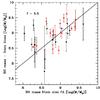 |
Fig. 3 Comparison of the BH mass estimates. Estimates with the SE method against those from fitting the accretion disk SED. The black points are from Shaw et al. (2012), the red points are our estimates using line data from Shen et al. (2011), the blue cross refers to the estimate by Shang et al. (2007) corrected as mentioned in the text. No error was reported for this estimate. |
4.2. The f-factor
The BH masses estimated with the SE method assume that the optical/UV line emission is coming mainly from the BLR, located at a radial distance RBLR from the central BH. When assuming that the BLR clouds are in virial equilibrium, M• is given by Eq. (1). There are two commonly used measures of the cloud velocity ΔV: the line FWHM and the dispersion of its Gaussian fit. We adopt the second one, ΔV = σline. RBLR is estimated using empirical analytic relations with continuum or line luminosities. With these assumptions and notation for an isotropic velocity field, we have f = 3 (Netzer 1990). This is, however, an oversimplified model. In practice, the value of f is empirically determined, but there is no consensus on its value (see Park et al. 2012a,b, and references therein). Values claimed in the literature differ by a factor of 2, from f ≃ 2.8 (Graham et al. 2011) to f ≃ 5.5 (Onken et al. 2004). For face-on objects (such as FSRQs), the average virial coefficient f may be larger than for optically selected QSOs (with random orientations) if the BLR has a flattened geometry (Decarli et al. 2011). The empirical relations used by Shen et al. (2011) and Shaw et al. (2012) implicitly assume f = 5.5, since this value was used, following Onken et al. (2004), in calibrating the reverberation mapping BH masses, which in turn were used as standards to calibrate SE mass estimators. Shang et al. (2007) followed a different approach by adopting f = 3. They also used a slightly different cosmology. We have corrected their BH mass estimate to homogenize it with the others.
4.3. Comparison of BH mass estimates
Thirty-four of the 54 blazars for which we could derive the BH masses with the blue bump fitting method also have published estimates with the SE method. In Fig. 3 we compare the results from the two methods, after having homogenized the SE estimates as described above. They are well correlated: the Spearman test yields a 99.96% (i.e. 3.5σ) significance for the correlation. The SE method with f = 5.5 yields, on average, slightly higher values of M•. We find an average ⟨ log (M•,SE/M•,blue bump) ⟩ = 0.09 with an rms dispersion of 0.40 dex. For comparison, the uncertainty of the SE method is 0.4−0.5 dex (Vestergaard & Peterson 2006; Park et al. 2012b) and that of the blue bump method is ≳0.2−0.4 (see Sect. 3). Thus the rms difference is fully accounted for by the uncertainties of the two methods. The offset between the two estimates would be removed setting f = 4.5, well within the range of current estimates. However, in view of the large uncertainties, reading this as an estimate of f would constitute an overinterpretation of the data. On the other hand, the consistency of the two methods strongly suggests that neither is badly off.
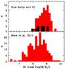 |
Fig. 4 Distributions of BH masses. The upper panel shows in red the distribution for our 54 objects having estimates via blue bump fitting and, in black, for 10 additional objects in the sample for which we have BH mass estimates via the SE method, homogenized as described in the text and decreased by 0.09 dex to remove the mean offset with blue bump estimates. The lower panel shows the distribution for all 1LAC blazars (Shaw et al. 2012) with masses decreased by 0.09 dex. |
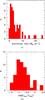 |
Fig. 5 Distributions of the accretion rate a) and of the Eddington ratio b) for the our FSRQs with evidence of a blue bump. |
4.4. Distribution of BH masses
In the upper panel of Fig. 4 we report the distribution of BH masses obtained by means of the blue bump fitting for 54 of our FSRQs and the distribution for the ten additional ones for which only SE estimates are available. The estimates for the latter objects have been first homogenized as described above and then decreased by 0.09 dex to correct for the mean offset with the blue bump results. The lower panel shows, for comparison, the distribution for 1LAC blazars in the Shaw et al. (2012) sample, again decreasing the BH masses by 0.09 dex. Whenever Shaw et al. (2012) provide more than one mass estimate for a single object we made a choice abiding by the order of preference mentioned in Sect. 4.1.
The figure shows that our 64 FSRQs are associated with very massive BHs (M• ≳ 107.8 M⊙) with a median value of 6.8 × 10⁸ M⊙. The median BH mass changes little (it becomes 7.4 × 10⁸ M⊙) if we restrict ourselves to the 54 FSRQs with BH mass estimates via blue bump fitting. The decline in the distribution at lower masses may be a selection effect: we selected radio-bright objects (S23 GHz ≥ 1 Jy) and the 15 (19%) FSRQs in our sample that neither show a detectable blue bump nor have SE estimates of the BH mass may well be associated with lower values of M•. On the other hand, our results are also consistent with the theoretical and observational studies that suggest that radio loud AGNs are generally associated with the most massive BHs (M• ≳ 108 M⊙, e.g., Chiaberge & Marconi 2011). The fast decline of the distribution above M• ≃ 109.4 M⊙, which suggests some upper bound to BH masses, is more likely to be real.
The BH mass distribution of Shaw et al. (2012) blazars adds support to the conclusion that blazar BH masses either below M• ~ 107.4 M⊙ or above M• ~ 109.6 M⊙ are rare. In this context, it is worth noticing that errors in BH mass estimates tend to populate the tails of the distribution by an effect that is analogous to the Eddington bias: objects tend to move from highly populated to less populated regions. Thus in particular the highest mass tail may be overpopulated (while the effect on the low-mass tail may be swamped by selection effects).
In Fig. 5 we report the distributions of the accretion rates (top panel) and of the Eddington ratios (bottom panel) for the 54 FSRQ in the sample for which we have estimated the BH mass fitting the blue bump of the spectrum, as reported in Table 2. We find a median Eddington ratio of 0.16 and a median accretion rate of 2.8 M⊙ yr-1. The few extreme values of these parameters must be taken with special caution on account of the uncertainties affecting our estimates.
The BH mass turns out to be anticorrelated with the disk peak frequency. Spearman’s test gives a probability of the null hypothesis (no correlation) p = 6.8 × 10⁻⁵. The anticorrelation follows from Eq. (5) due to the weak dependence of M• on the accretion rate and the limited range of Ṁ spanned by our blazars.
5. Discussion and conclusions
We have compared BH mass estimates based on fitting the blue bump with a Shakura & Sunyaev (1973) model with those obtained with the commonly used single-epoch virial method (SE method) for a complete sample of FSRQs drawn from the WMAP 7 yr catalog, all with measured spectroscopic redshift. The sample comprises 79 objects with S23 GHz ≥ 1 Jy, 54 of which (68%) have a clearly detected “blue bump” from which the BH mass could be inferred. FSRQs are the AGN population best suited to such a comparison because there is strong evidence that their jets are highly aligned with the line-of-sight, suggesting that the accretion disk should be almost face-on, thus minimizing the uncertainty on the inclination angle that bewilders BH mass estimates for the other AGN populations.
The mass estimates obtained from the two methods are well correlated. If the calibration factor f of the SE relation, (Eq. (1)), is set to f = 4.5, well within the range of recent estimates, the mean logarithmic ratio of the two mass estimates is ⟨ log (M•,SE/M•,blue bump) ⟩ = 0 and its dispersion is 0.40, which is close to what is expected from uncertainties of the two methods. That the two independent methods agree so closely in spite of all the potentially large uncertainties associated with each (see Sects. 1 and 3) lends strong support to both of them; however, the agreement is only statistical, and individual estimates of BH masses must be taken with caution.
The distribution of BH masses for the 54 FSRQs in our sample with a well-detected blue bump has a median value of 7.4 × 10⁸ M⊙. It declines at the low-mass end, consistent with other indications that radio-loud AGNs are generally associated with the most massive BHs, although the decline may be, at least partly, due to the source selection. The distribution drops above M• = 2.5 × 10⁹ M⊙, implying that ultra-massive BHs associated with FSRQs must be rare.
According to the WISE Explanatory Supplement (Cutri et al. 2013), sources with S/N ~ 20 have a typical rms positional uncertainty of 0.43 arcsec. Our sources generally have a much lower S/N ratio and the astrometric uncertainty scales as (S/N)-1 (e.g. Condon et al. 1998; Ivison et al. 2007). For the typical S/N values of our sources, S/N = 3−5, the search radius correspond to positional errors in the range 2.3−3.8σ.
Acknowledgments
We gratefully acknowledge very useful comments from an anonymous referee. This work was supported in part by ASI/INAF agreement n. I/072/09/0 and by INAF through the PRIN 2009 “New light on the early Universe with sub-mm spectroscopy”. This publication has made use of data products from the Wide-field Infrared Survey Explorer, which is a joint project of the University of California, Los Angeles, and the Jet Propulsion Laboratory/California Institute of Technology, funded by the National Aeronautics and Space Administration, and of the NASA/IPAC Extragalactic Database (NED), which is operated by the Jet Propulsion Laboratory, California Institute of Technology, under contract with the National Aeronautics and Space Administration.
References
- Abazajian, K., Adelman-McCarthy, J. K., Agüeros, M. A., et al. 2004, AJ, 128, 502 [Google Scholar]
- Abdo, A. A., Ackermann, M., Ajello, M., et al. 2010, ApJ, 715, 429 [NASA ADS] [CrossRef] [Google Scholar]
- Ajello, M., Shaw, M. S., Romani, R. W., et al. 2012, ApJ, 751, 108 [NASA ADS] [CrossRef] [Google Scholar]
- Assef, R. J., Frank, S., Grier, C. J., et al. 2012, ApJ, 753, L2 [NASA ADS] [CrossRef] [Google Scholar]
- Bentz, M. C., Peterson, B. M., Pogge, R. W., & Vestergaard, M. 2009, ApJ, 694, L166 [NASA ADS] [CrossRef] [Google Scholar]
- Blandford, R. D., & McKee, C. F. 1982, ApJ, 255, 419 [NASA ADS] [CrossRef] [EDP Sciences] [Google Scholar]
- Calderone, G., Ghisellini, G., Colpi, M., Dotti, M., 2013, MNRAS, 431, 210 [NASA ADS] [CrossRef] [Google Scholar]
- Cardelli, J. A., Clayton, G. C., & Mathis, J. S. 1989, ApJ, 345, 245 [NASA ADS] [CrossRef] [Google Scholar]
- Cash, W. 1976, A&A, 52, 307 [NASA ADS] [Google Scholar]
- Chiaberge, M., & Marconi, A. 2011, MNRAS, 416, 917 [NASA ADS] [CrossRef] [Google Scholar]
- Condon, J. J., Cotton, W. D., Greisen, E. W., et al. 1998, AJ, 115, 1693 [NASA ADS] [CrossRef] [Google Scholar]
- Croom, S. M. 2011, ApJ, 736, 161 [NASA ADS] [CrossRef] [Google Scholar]
- Cutri, R. M., Wright, E. L., Conrow, T., et al. 2013, wise2.ipac.caltech.edu/docs/release/allsky/expsup/ [Google Scholar]
- Decarli, R., Dotti, M., & Treves, A. 2011, MNRAS, 413, 39 [NASA ADS] [CrossRef] [Google Scholar]
- Donato, D., Ghisellini, G., Tagliaferri, G., & Fossati, G. 2001, A&A, 375, 739 [NASA ADS] [CrossRef] [EDP Sciences] [Google Scholar]
- Ferrarese, L., & Ford, H. 2005, Space Sci. Rev., 116, 523 [NASA ADS] [CrossRef] [Google Scholar]
- Frank, J., King, A., & Raine, D. J. 2002, Accretion Power in Astrophysics, 3d edn., eds. J. Frank, A. King, & D. Raine (Cambridge, UK: Cambridge University Press) [Google Scholar]
- Ghisellini, G., Della Ceca, R., Volonteri, M., et al. 2010, MNRAS, 405, 387 [NASA ADS] [Google Scholar]
- Giommi, P., Polenta, G., Lähteenmäki, A., et al. 2012, A&A, 541, A160 [NASA ADS] [CrossRef] [EDP Sciences] [Google Scholar]
- Gold, B., Odegard, N., Weiland, J. L., et al. 2011, ApJS, 192, 15 [Google Scholar]
- Graham, A. W., Onken, C. A., Athanassoula, E., & Combes, F. 2011, MNRAS, 412, 2211 [NASA ADS] [CrossRef] [Google Scholar]
- Greene, J. E., & Ho, L. C. 2005, ApJ, 630, 122 [NASA ADS] [CrossRef] [Google Scholar]
- Haardt, F., & Madau, P. 2012, ApJ, 746, 125 [NASA ADS] [CrossRef] [Google Scholar]
- Hancock, P. J., Roberts, P., Kesteven, M. J., et al. 2011, Exp. Astron., 32, 147 [NASA ADS] [CrossRef] [Google Scholar]
- Hinshaw, G., Weiland, J. L., Hill, R. S., et al. 2009, ApJS, 180, 225 [NASA ADS] [CrossRef] [Google Scholar]
- Ivison, R. J., Greve, T. R., Dunlop, J. S., et al. 2007, MNRAS, 380, 199I [NASA ADS] [CrossRef] [Google Scholar]
- Kaspi, S., Smith, P. S., Netzer, H., et al. 2000, ApJ, 533, 631 [NASA ADS] [CrossRef] [Google Scholar]
- Kaspi, S., Maoz, D., Netzer, H., et al. 2005, ApJ, 629, 61 [NASA ADS] [CrossRef] [Google Scholar]
- Koratkar, A. P., & Gaskell, C. M. 1991, ApJ, 370, L61 [NASA ADS] [CrossRef] [Google Scholar]
- Laor, A. 1990, MNRAS, 246, 369 [NASA ADS] [Google Scholar]
- Li, L.-X., Zimmerman, E. R., Narayan, R., & McClintock, J. E. 2005, ApJS, 157, 335 [NASA ADS] [CrossRef] [Google Scholar]
- Malkan, M. A. 1983, ApJ, 268, 582 [NASA ADS] [CrossRef] [Google Scholar]
- Mannucci, F., Basile, F., Poggianti, B. M., et al. 2001, MNRAS, 326, 745 [NASA ADS] [CrossRef] [Google Scholar]
- Massaro, E., Giommi, P., Leto, C., et al. 2011, Multifrequency Catalogue of Blazars, 3rd edn. (Rome: ARACNE Editrice) [Google Scholar]
- Morrissey, P., Conrow, T., Barlow, T. A., et al. 2007, ApJS, 173, 682 [NASA ADS] [CrossRef] [Google Scholar]
- Netzer, H. 1990, in Saas-Fee Advanced Course 20: Active galactic nuclei, 57 [Google Scholar]
- O’Donnell, J. E. 1994, ApJ, 422, 158 [NASA ADS] [CrossRef] [Google Scholar]
- Onken, C. A., Ferrarese, L., Merritt, D., et al. 2004, ApJ, 615, 645 [NASA ADS] [CrossRef] [Google Scholar]
- Park, D., Kelly, B. C., Woo, J.-H., & Treu, T. 2012a, ApJS, 203, 6 [NASA ADS] [CrossRef] [Google Scholar]
- Park, D., Woo, J.-H., Treu, T., et al. 2012b, ApJ, 747, 30 [Google Scholar]
- Planck Collaboration 2011a, A&A, 536, A7 [NASA ADS] [CrossRef] [EDP Sciences] [Google Scholar]
- Planck Collaboration 2011b, A&A, 536, A13 [NASA ADS] [CrossRef] [EDP Sciences] [Google Scholar]
- Polletta, M., Tajer, M., Maraschi, L., et al. 2007, ApJ, 663, 81 [NASA ADS] [CrossRef] [Google Scholar]
- Schneider, D. P., Richards, G. T., Hall, P. B., et al. 2010, AJ, 139, 2360 [NASA ADS] [CrossRef] [Google Scholar]
- Shakura, N. I., & Sunyaev, R. A. 1973, A&A, 24, 337 [NASA ADS] [Google Scholar]
- Shang, Z., Wills, B. J., Wills, D., & Brotherton, M. S. 2007, AJ, 134, 294 [NASA ADS] [CrossRef] [Google Scholar]
- Shankar, F., Weinberg, D. H., & Miralda-Escudé, J. 2009, ApJ, 690, 20 [NASA ADS] [CrossRef] [Google Scholar]
- Shaw, M. S., Romani, R. W., Cotter, G., et al. 2012, ApJ, 748, 49 [CrossRef] [Google Scholar]
- Shen, Y. 2013, Bull. Astron. Soc. India, 41, 61 [NASA ADS] [Google Scholar]
- Shen, Y., Richards, G. T., Strauss, M. A., et al. 2011, ApJS, 194, 45 [NASA ADS] [CrossRef] [Google Scholar]
- Trushkin, S. A. 2003, Bull. Special Astrophys. Obs., 55, 90 [Google Scholar]
- Vestergaard, M., & Peterson, B. M. 2006, ApJ, 641, 689 [NASA ADS] [CrossRef] [Google Scholar]
- Wandel, A., & Petrosian, V. 1988, ApJ, 329, 11 [Google Scholar]
- Wright, E. L., Eisenhardt, P. R. M., Mainzer, A. K., et al. 2010, AJ, 140, 1868 [NASA ADS] [CrossRef] [Google Scholar]
- Wu, X.-B., Wang, R., Kong, M. Z., Liu, F. K., & Han, J. L. 2004, A&A, 424, 793 [NASA ADS] [CrossRef] [EDP Sciences] [Google Scholar]
All Tables
Redshift-dependent effective optical depth for IGM absorption, averaged over all lines of sight, at the effective wavelengths of the GALEX NUV and FUV bands and of SDSS the g and u bands.
All Figures
|
Fig. 1 Redshift-dependent effective optical depth for IGM absorption, averaged over all lines of sight, at the effective wavelengths of SDSS g and u bands and of the GALEX NUV and FUV bands. |
| In the text | |
|
Fig. 2 Example of an SED fit (WMAP7 # 190). Solid blue parabola: total SED, which includes synchrotron emission, host galaxy, disk and torus emissions; dashed violet line: synchrotron from the jet; green dashed line: torus; dashed cyan line: host galaxy, taken to be a passive elliptical with MR = −23.7; dashed red line: accretion disk. Orange points: Planck data; green: WISE data; red: SDSS data; magenta: GALEX data. Black points: data taken from the NASA/IPAC Extragalactic Database (NED). At variance with what was done to compute Ld (see text), the luminosities shown here are computed assuming isotropic emission. |
| In the text | |
|
Fig. 3 Comparison of the BH mass estimates. Estimates with the SE method against those from fitting the accretion disk SED. The black points are from Shaw et al. (2012), the red points are our estimates using line data from Shen et al. (2011), the blue cross refers to the estimate by Shang et al. (2007) corrected as mentioned in the text. No error was reported for this estimate. |
| In the text | |
|
Fig. 4 Distributions of BH masses. The upper panel shows in red the distribution for our 54 objects having estimates via blue bump fitting and, in black, for 10 additional objects in the sample for which we have BH mass estimates via the SE method, homogenized as described in the text and decreased by 0.09 dex to remove the mean offset with blue bump estimates. The lower panel shows the distribution for all 1LAC blazars (Shaw et al. 2012) with masses decreased by 0.09 dex. |
| In the text | |
|
Fig. 5 Distributions of the accretion rate a) and of the Eddington ratio b) for the our FSRQs with evidence of a blue bump. |
| In the text | |
Current usage metrics show cumulative count of Article Views (full-text article views including HTML views, PDF and ePub downloads, according to the available data) and Abstracts Views on Vision4Press platform.
Data correspond to usage on the plateform after 2015. The current usage metrics is available 48-96 hours after online publication and is updated daily on week days.
Initial download of the metrics may take a while.