| Issue |
A&A
Volume 559, November 2013
|
|
|---|---|---|
| Article Number | A27 | |
| Number of page(s) | 17 | |
| Section | Extragalactic astronomy | |
| DOI | https://doi.org/10.1051/0004-6361/201321765 | |
| Published online | 31 October 2013 | |
Polarized synchrotron radiation from the Andromeda galaxy M 31 and background sources at 350 MHz⋆,⋆⋆
1 Max-Planck-Institut für Radioastronomie, Auf dem Hügel 69, 53121 Bonn, Germany
e-mail: rgiess@mpifr-bonn.mpg.de
2 ASTRON, PO Box 2, 7990 AA Dwingeloo, The Netherlands
3 Kapteyn Astronomical Institute, University of Groningen, PO Box 800, 9700 AV Groningen, The Netherlands
4 I. Physikalisches Institut, Universität zu Köln, Zülpicher Straße 77, 50937 Köln, Germany
5 Isaac Newton Institute of Chile, Armenian Branch, and Byurakan Astrophysical Observatory, Byurakan 378433, Armenia
Received: 24 April 2013
Accepted: 8 September 2013
Context. Low-frequency radio continuum observations are best suited to search for radio halos of inclined galaxies. Polarization measurements at low frequencies allow the detection of small Faraday rotation measures caused by regular magnetic fields in galaxies and in the foreground of the Milky Way.
Aims. The detection of low-frequency polarized emission from a spiral galaxy such as M 31 allows us to assess the degree of Faraday depolarization, which can be compared with models of the magnetized interstellar medium.
Methods. The nearby spiral galaxy M 31 was observed in two overlapping pointings with the Westerbork Synthesis Radio Telescope (WSRT), resulting in about 4′ resolution in total intensity and linearly polarized emission. The frequency range 310–376 MHz was covered by 1024 channels, which allowed the application of rotation measure (RM) synthesis on the polarization data. We derived a data cube in Faraday depth and compared two symmetric ranges of negative and positive Faraday depths. This new method avoids the range of high instrumental polarization and allows the detection of very low degrees of polarization.
Results. For the first time, diffuse polarized emission from a nearby galaxy is detected below 1 GHz. The degree of polarization is only 0.21 ± 0.05%, consistent with the extrapolation of internal depolarization from data at higher radio frequencies. A catalogue of 33 polarized sources and their Faraday rotation in the M 31 field is presented. Their average depolarization is DP(90,20) = 0.14 ± 0.02, which is seven times more strongly depolarized than at 1.4 GHz. We argue that this strong depolarization originates within the sources, for instance in their radio lobes, or in intervening galaxies on the line of sight. On the other hand, the Faraday rotation of the sources is mostly produced in the foreground of the Milky Way and varies significantly across the ~9 square degrees of the M 31 field.
Conclusions. As expected, polarized emission from M 31 and extragalactic background sources is much weaker at low frequencies than in the GHz range. Future observations with LOFAR, with high sensitivity and high angular resolution to reduce depolarization, may reveal diffuse polarization from the outer disks and halos of galaxies.
Key words: instrumentation: interferometers / techniques: polarimetric / galaxies: individual: M 31 / galaxies: magnetic fields / radio continuum: galaxies
Appendices are available in electronic form at http://www.aanda.org
The RM synthesis datacube is only available at the CDS via anonymous ftp to cdsarc.u-strasbg.fr (130.79.128.5) or via http://cdsarc.u-strasbg.fr/viz-bin/qcat?J/A+A/559/A27
© ESO, 2013
1. Introduction
The Andromeda galaxy (M 31) at a distance of ~750 kpc1 was one of the first external spiral galaxies from which polarized radio emission was detected (Beck et al. 1978). Most of the radio continuum emission is synchrotron emission, originating from cosmic-ray electrons that spiral around the interstellar magnetic field lines. An early analysis of the polarized emission showed that the turbulent and ordered components of the magnetic field are concentrated in a ring-like structure at about 10 kpc radius (Beck 1982). This ring is a superposition of several spiral arms with small pitch angles, seen under the inclination of 75° (Chemin et al. 2009). Faraday rotation measures (RM) showed that the ordered field of M 31 is coherent, meaning that it preserves its direction around 360° in azimuth and across several kiloparsecs in radius (Beck 1982; Berkhuijsen et al. 2003). This large-scale field can be traced out to about 20 kpc distance from the centre of M 31, using polarized background sources in the M 31 field as an RM grid (Han et al. 1998).
By now we know that spiral (and even some irregular) galaxies exhibit ordered magnetic fields (Beck 2005) with average field strengths of 5 ± 3 μG, while the average random field is typically three times stronger (assuming energy equipartition between magnetic fields and cosmic rays) (Fletcher 2010). In M 31 the strengths of the ordered and random fields are about equal (5 ± 1 μG) (Fletcher et al. 2004), which is unique among the galaxies observed so far.
These ordered fields on scales of the entire galaxy can be best explained by dynamo theory (Beck et al. 1996). It requires weak magnetic seed fields and an interplay of turbulence and shear to generate and maintain such a field. The turbulence can be provided by supernova explosions, while shear is a consequence of the differential rotation of the galactic disk. The exceptionally well ordered large-scale magnetic field in M 31 can be well described by an axisymmetric spiral pattern, the basic dynamo mode m = 0, disturbed by a weaker m = 2 mode (Fletcher et al. 2004). The magnetic field in M 31 is the prototypical case of a dynamo-generated field.
To our knowledge, there has been no detection of diffuse polarization from spiral galaxies below 1 GHz. All observations of polarization from nearby galaxies were restricted to the GHz range so far. Lower frequencies are advantageous in several aspects: (1) synchrotron emission is stronger, especially from steep-spectrum radio halos, and (2) Faraday rotation is stronger, allowing the measurement of small RM even with low signal-to-noise ratios. Multichannel polarimetry allows the application of RM synthesis (Brentjens & de Bruyn 2005), which generates Faraday spectra for each map pixel. The achieved resolution in Faraday spectra increases with coverage in λ2 space (Δλ2) and hence is higher at low frequencies. On the other hand, Faraday depolarization increases towards lower frequencies at a rate depending on the depolarization mechanism (Burn 1966; Sokoloff et al. 1998; Tribble 1991). As a result, polarized emission decreases below some characteristic frequency that depends on the properties of the Faraday-rotating medium (Arshakian & Beck 2011). Depolarization in M 31 is relatively low because of its weak turbulent magnetic field (Sect. 5.3). This makes M 31 an excellent candidate for low-frequency polarization studies.
The properties of nearby galaxies as observed in radio continuum below 250 MHz will soon be explored with the LOw Frequency ARray (LOFAR, van Haarlem et al. 2013), to search for extended synchrotron emission far away from the galactic disks and in the galactic halos. The observations at 350 MHz presented in this paper are a crucial observational link between observations at gigahertz frequencies and the upcoming observations with LOFAR. To this point, the polarization properties of galactic disks and the feasibility to use polarized point sources as a background grid to explore magnetic fields in the foreground are untested at low frequencies.
2. Observations
M 31 was observed on four different days using the WSRT in December 2008. Two pointings centred at RA = 00h45m00.0s, Dec = 41d49m59.9s and RA = 00h41m00.0s, Dec = 40d46m00.1s were required to cover the entire galaxy. The maxi-short configuration was used, which is optimized for imaging performance. The shortest baselines in this configuration are 36 m, 54 m, 72 m, and 90 m. Each of the two pointings was observed for 2 × 12 h.
For each 12 h pointing four calibrators were observed: 3C 295 for flux calibration and 3C 303 for polarization calibration at the beginning and 3C 147 for flux calibration and DA240 as polarization calibrator at the end.
During the observations the correlator produced 128 channels with a channel width of 78.125 kHz for each of the eight frequency bands in all four cross correlations (XX, XY, YX, YY) with 60 s integration time. The bands (also denoted IFs for intermediate frequencies) were centred on 315.0 MHz, 323.75 MHz, 332.5 MHz, 341.25 MHz, 350.0 MHz, 358.75 MHz, 367.5 MHz, and 376.25 MHz.
After flagging of channels corrupted by radio frequency interference (RFI, see below) the resulting mean frequency of this observation is 343.4 MHz, which corresponds to λ87.3 cm, called 90 cm throughout this paper.
3. Data reduction
Calibration was made in CASA 3.3.0 (Common Astronomy Software Applications)2 after correcting for the system temperature in AIPS (Astronomical Image Processing System)3. For low-frequency observations with the WSRT there are some limitations of the standard CASA tasks, but since the software is based on the script language python, the user has total control over the data and can also run tasks in batch mode. This is important, since calibration and imaging has to be performed for each channel separately. Due to the large number of channels, this has to be automated.
3.1. Flagging
With this amount of data, manual flagging of every single channel is no longer possible. The software package rficonsole by Offringa et al. (2010) was used, which was specifically developed for low-frequency data of LOFAR and the WSRT. The algorithm is described in Offringa et al. (2010). It features a general user interface, with which one can inspect the data manually. Here one develops a so-called strategy (essentially a parameter file used by rficonsole), by randomly checking for single baselines how well the algorithm detects any RFI.
Since the bandpass response across a spectral window is filtered and drops smoothly to zero at the edges to reduce aliasing effects, a bandpass calibration is performed beforehand to facilitate the operation of the algorithm. Rficonsole is applied to the bandpass-corrected data in the CORRECTED_DATA column, but the flags are stored in a separate table and are also applied to the DATA column, which holds the raw data and is used for the following steps. The final bandpass calibration is made after the flagging. The first 3 and last 17 channels of all IFs are unusable due to the anti-aliasing filter and are flagged as well. Since the bands overlap, one does in general not lose any frequency channels.
However, here two of the bands, IF2 and IF3 (358.75 MHz and 350.0 MHz) were unusable due to RFI and had to be removed entirely for all four days.
Because the maxi-short configuration was used for the observation, antennas RT9 and RTA were subject to shadowing4. RT9 was manually flagged for hour angles ≦− 5h, RTA for hour angles ≧+5h.
3.2. Calibration
The system temperature (Tsys) calibration had to be performed in AIPS, since CASA 3.3.0 was unable to read the Tsys information table provided from the telescope. However, for the calibration in AIPS, the polarization products have to be transformed from linear polarization (XX, XY, YX, YY) to circular polarization (RR, LL, RL, LR). Detailed instructions are given in the CookBook for WSRT data reduction using classic AIPS by R. Braun5.
The observation of 3C 295 and 3C 303 failed on the second day. For consistency only 3C 147 and DA240 were used for calibration. Where possible, the gain solutions were applied to 3C 295 and 3C 303 to check their validity.
The flux of 3C 147 was derived using the analytic function given in the VLA Calibrator Manual6 (Perley & Taylor 2003),  (1)with A = 1.44856,B = −0.67252,C = −0.21124,D = + 0.04077. At the time of writing, more precise models for the six most common calibrators at low frequencies were published by Scaife & Heald (2012). For 3C 147 both models agree well within the uncertainties, but the spectrum is probably slightly steeper in our frequency range. The deviation is lower than 3%, therefore we did not need to repeat the entire data reduction.
For DA240 the values published in Brentjens (2008) were assumed: RM = + 3.33 ± 0.14 rad m-2 and a polarization angle at λ2 = 0 of pa = 122° ± 3°.
At these wavelengths 3C 303 is expected to be 5% polarized with an RM of +15 rad m-2 (Ger de Bruyn, priv. comm.). This value differs slightly from (but still agrees with) the published value of RM = + 18 ± 2 rad m-2 at GHz frequencies (Simard-Normandin et al. 1981).
The results of calibrating 3C 303 confirm that the polarization calibration remains constant over the 12 h of each observation, which means that the ionosphere was reasonably stable during this time span. In December 2008, solar activity was near a minimum, ionospheric Faraday rotation is thus expected to be only a few rad m-2 and stable, which means that any effects can be handled by the calibration.
The calibration has to be made for each channel individually, solving for all elements in the Jones matrices (Hamaker et al. 1996), to circumvent problems caused by the so-called 17 MHz ripple. This is a variation of the gains with frequency (at a period of 17 MHz), caused by a standing wave between the dish and the primary focus of the antennas. It sometimes results in strong frequency-dependent variations in the spectra of off-axis sources across the primary beam and polarization leakages (Popping & Braun 2008; Brentjens 2008).
The properties of the calibrators (namely the expected values for the four Stokes parameters) were calculated for each channel independently and were written into the MODEL_DATA column of the measurement set. Afterwards the CASA tasks gaincal, polcal, and applycal were used to calculate and apply the gains to the other calibrators and the M 31 fields. This was done separately for each channel and each of the four observations.
3.3. Selfcal, peeling, and imaging
Several rounds of self-calibration (selfcal) were performed before final imaging of the visibility (uv) data of M 31. A single selfcal step consists of imaging and cleaning the uv data to obtain a clean model of the field and using that clean model for calculatin and applying gain solutions to the field. But first Cassiopeia A and Cygnus A had to be removed from the data, since during imaging side-lobes from both sources were visible within the M 31 field. The two sources are far away from the pointing centre, but they are the brightest sources in the sky at these frequencies.
Sources can be subtracted from the uv data using the so-called peeling method. This is a general method for removing off-axis sources from the field, for which good gain solutions cannot be derived with normal selfcal. It requires the following steps:
-
1.
Obtain a good clean model of the observed field. Usually aselfcal step (excluding the source(s) to be subtracted) isperformed to be able to produce a better clean-model.
-
2.
Subtract that model from the uv data. This step is performed so that no side-lobes from the field interfere with the source that is to be peeled. If a selfcal step was made, the model has to be subtracted from the CORRECTED_DATA column. Since the gain-solutions from the selfcal step did not include the source that is being peeled, they will be entirely wrong for this source. Thus, after subtracting the calibration with the field sources has to be reversed by inverting the gain table and applying the inverted gains.
-
3.
Use the field-subtracted uv data to obtain a good clean model of the source that is to be peeled. Usually this involves setting the phase centre to the position of the source, and again performing selfcal on the source in question.
-
4.
Subtract the new model from the original uv data. If selfcal was used, first apply the gain solutions, then subtract and reverse the calibration by again applying the inverted gains.
For better results, this can be repeated in an iterative process, since the model for the field will improve after the disturbing influences of the peeled source are reduced, leading to a better subtraction and thus a better model for the source to be peeled, and so on.
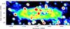 |
Fig. 1 Final total power image of M 31 at 90 cm. Contours are from 4 to 128 mJy/beam in steps of 10 mJy/beam. HPBW: 230′′ × 290′′; rms = 1.4 mJy/beam. The black crosses mark the pointing centres of the two fields. Note: the tick marks may be misleading since the map is rotated with respect to the celestial coordinates, see the coordinate grid in Fig. 2 or Fig. 4. |
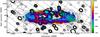 |
Fig. 2 Spectral index (SI) map between 90 cm and 20 cm overlaid with the same contours as Fig. 1. The SI map was calculated for intensities >5σ in Stokes I. |
Here it was sufficient to run selfcal on the field using only the brightest sources, subtract that model from the field, apply the inverted gains from the selfcal and then subtract Cassiopeia A and afterwards subtract Cygnus A without any selfcal steps. (Both sources are too far away from the original phase-centre to achieve any good solutions.)
After peeling, three selfcal runs were performed on each M 31 field (again separately for each channel and each of the four days). For the initial model, the uv range was restricted to baselines >0.1 kλ to exclude the extended emission and start with a simple model. Only the brightest sources and uniform weighting were used. The resulting image was cleaned to three times the noise-level measured in the Stokes V image for each channel individually. In the second run the uv range was still restricted, and more sources as well as the bright centre of M 31 were included. The threshold for cleaning was reduced to twice the noise. In the final step the uv range was no longer restricted and the entire M 31 was included in the model and cleaned down to the noise-level.
This procedure was tested for different channels across the entire bandwidth and then automated with python to run without user-interaction for each channel separately.
3.4. Final imaging
For the final images the uv range was restricted from 34.5 λ to 2801.0 λ. This is the maximum uv range that all channels have in common, and ensures that for all frequencies the spatial resolution is the same. The images for all four Stokes parameters were cleaned automatically using Briggs-weighting and a uv taper and afterwards were slightly smoothed to a final resolution of 230′′ × 290′′. The Stokes Q and U images are then used for RM synthesis (Sect. 5).
For the total power map, the channels were once again inspected using the images from the automatic imaging run, and obviously bad channels were excluded. Then the uv data was concatenated per field and per IF, keeping the individual channels, and imaged manually, resulting in one image per field and per IF. As a last imaging step the two fields had to be mosaicked and primary-beam corrected.
3.4.1. Primary-beam correction and mosaicking
According to the ASTRON webpage, the primary beam response can be described by the function7 (2)where r is the distance from the pointing centre in degrees and ν the observing frequency in GHz. The automatic primary beam correction in CASA uses a different function for the WSRT. The constant c is only constant for GHz frequencies and is said to decline to c = 66 at 325 MHz and c = 63 at 4995 MHz. It is related to the light crossing time across the aperture (i.e. the effective diameter of the dish, Brentjens 2008). A good primary beam correction is crucial in our case, because M 31 spans two pointings. Since there is no exact value given and recommendations vary (e.g. c = 64, Ger de Bruyn, priv. comm.), we manually determined the best value for our observation.
For four arbitrary chosen channels across all bands (IF 0, channel 15; IF 1, channel 83; IF 5, channel 26; and IF 7 channel 57), the primary-beam correction was applied for different values of c. Then the difference between the peak fluxes of each of the ten sources in the overlap area of the primary beams between the northern and southern field at the same frequency was calculated and normalized to the flux density in the northern field,  (3)Hence, for each constant c there are ten values fi(c) (per chosen channel) between −1 and +1. For a perfect primary-beam correction, each value would be equal to 0. The error in the mean of these ten values is thus a measure for the quality of the primary beam correction,
 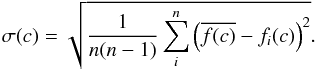 (4)For c = 65, all the systematic errors are at their lowest common point and are also all below 10%, which is deemed an acceptable level. Using this value for the primary beam correction, the resulting systematic flux error was estimated to be 7 − 8%.
Mosaicking was made in the image domain, using a standard linear mosaicking scheme (see Cornwell et al. 1993; Sault et al. 1996), assuming equal noise levels for both fields, 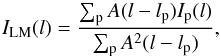 (5)where A(l − lp) is the primary beam attenuation at distance l from the pointing centre lp (Eq. (2)) and Ip is the cleaned image of the respective field.
4. Total emission from M 31 at 90 cm
The final total power image is shown in Fig. 1. It is a uniformly weighted average of the single IF images (see Sect. 3.4). Note that even at these low frequencies, no excess radio continuum emission (i.e. a radio halo) is detected around M 31. This has already been inferred by Gräve et al. (1981).
After subtracting all sources <0.1 Jy, we found a total flux density integrated over the radius interval R = 0 − 17.4 kpc 8 of 10.6 ± 0.7 Jy. The error is estimated from the standard deviation of the total fluxes for M 31 for the individual IF images. The value is consistent with the integrated flux densities listed by Berkhuijsen et al. (2003). We note that the value may be slightly too low due to missing spacings. After restricting the UV range (see Sect. 3.4), our largest detectable structure is 1.7°. This would still enable us to detect a halo along the minor axis.
Figure 2 shows a spectral index (SI) map between our 90 cm map and the VLA+Effelsberg 20 cm map by Beck et al. (1998). The spectral index is very similar to that presented by Berkhuijsen et al. (2003) between 20 cm and 6 cm. Like at GHz frequencies, we found on average a slightly steeper spectral index towards the southern major axis (α90,20 ≈ − 0.7) compared with the northern major axis (α90,20 ≈ − 0.6). The north-eastern part of the ring (lower left in Fig. 2) is dominated by Hii regions and shows a flat spectral index of only α90,20 ≈ − 0.4. This is even flatter than the average value found in the SI map by Berkhuijsen et al. (2003) at GHz frequencies. With a constant thermal fraction and a constant nonthermal spectral index one would expect the spectral index to steepen at low frequencies, so this indicates that thermal absorption is considerable. We note that missing spacings are no problem for the spectral index here, since they only become significant in the faint outermost regions. The overall spectral index, dominated by the bright regions, is therefore not affected.
A more thorough analysis would require a higher resolution map at 90 cm to allow proper subtraction of all point sources and is beyond the scope of this paper.
5. Polarized emission and RM synthesis
The Faraday depth (FD) is proportional to the integral along the line of sight over the cosmic-ray electron density ne and the strength of the line of sight component of the regular magnetic field B (Burn 1966), 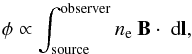 (6)while the classical RM is an observable quantity that describes the difference of polarization angles Δχ observed at two (or more) different wavelengths λi,
 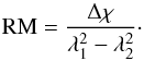 (7)The classical RM is equivalent to the FD φ only if there is just a background source and a dispersive Faraday screen in the foreground along the line of sight. If there are several emitting and rotating components along the line of sight, the linear relationship between Δχ and Δ(λ2) in Eq. (7) does not hold. In addition, there is an ambiguity because the polarization vector could have rotated by nπ (n a natural number) without being noticed.
RM synthesis, on the other hand, yields a spectrum F(φ) in FD φ, in which each polarization-emitting component along the line of sight will produce a separate signal. Its position in FD corresponds to the total rotation of the rotating components between the emitting component and the observer along the line of sight (see Fig. 3). For more details on RM synthesis we refer to Brentjens & de Bruyn (2005) and Heald (2009).
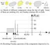 |
Fig. 3 Example for a set of different polarization-emitting and rotating components along the line of sight and the resulting Faraday spectrum. E1 and E3 are point sources, E2,R2 is an extended emitting and rotating region. R1, R3, and R4 are Faraday screens that are not emitting. Depolarization effects are neglected here for simplicity. |
5.1. RM synthesis at 90 cm
RM synthesis was performed on the automatically cleaned Q and U images after mosaicking, using the software by Michiel Brentjens (Brentjens & de Bruyn 2005; Brentjens 2008). The resulting Faraday cube was then cleaned using the RM Clean code for MIRIAD (Sault et al. 1995) implemented by one of us (GH; Heald et al. 2009, using 1σ as cutoff level and nmax = 1000. RM clean converged after ~975 iterations.
The resolution in FD φ of our observation is given by the measured full width at half maximum of the RM spread function (RMSF) ϕ = 19.12 rad m-2. The largest detectable structure in Faraday space is  rad m-2.
Note that the terms RM clean and RMSF are misleading because only in exceptional cases RM and FD φ are the same (see above).
5.2. Polarized sources
5.2.1. Catalogue
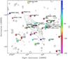 |
Fig. 4 Position and Faraday depth of the detected sources on contours of the total power map. |
We compiled a catalogue of all (33) polarized sources detected in the Faraday cube in Table A.1. The listed positions correspond to the brightest, central pixel of that source in the image plane at the FD it was detected. The polarized intensities (PI) are the peak intensities in the Faraday cube, and each polarization degree (p) was calculated with the respective intensity at that position in the Stokes I map. The name of the corresponding source from the Walterbos et al. (1985) catalogue and/or from Taylor et al. (2009) is given if the source is listed. If marked with a “?” the assignment is not entirely certain because the position of the peak and that in the catalogue differ slightly. This can occur because of uncertainties due to the low resolution in the WSRT data, sources consisting of several unresolved components, or in fact an erroneous assignment. For comparison the polarization properties measured at 1.4 GHz (21 cm) by Han et al. (1998) and Taylor et al. (2009) are listed where available. We note that only nine of the 21 sources listed by Han et al. (1998) were detected at 90 cm. The FD derived from RM synthesis at 90 cm is denoted by φ, whereas RM denotes Faraday rotation measures obtained from two frequency bands.
The average value of φ of all sources in the catalogue is − 67 ± 40 rad m-2 (where ± 40 rad m-2 is the standard deviation). The average degree of polarization is 1.36%. Most values are below 3%; only five sources are more strongly polarized.
An important selection criterion for a source to be included in the catalogue was a clear recognition as a point-like source in the cube. Plots of the FD along slices through the source positions in RA/Dec are a good tool for determining the spatial extent of peaks in the Faraday cube. In Appendix B the Faraday spectra of all detected sources are shown. The polarization data (Figs. B.1 to B.6) is available in FITS format at the CDS. Some have several components, but these peaks belong to extended structures in the cube that are unrelated to M 31 (Sect. 5.3). The error in FD is estimated by 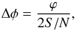 (8)where ϕ is the full width at half maximum of the RMSF and S/N the signal-to-noise ratio of the peak. This is a similar error estimation as is used for source detection in imaging (e.g. Fomalont 1999). The error in polarized intensity is the noise level of the Faraday cube, which is about 1/
 times lower than the rms in the single Q and U images (Nchan is the number of frequency channels). The lowest S/N > 8, therefore polarization-bias correction can be neglected.
Figure 4 shows the position of the detected sources on contours of the total power map. The colour corresponds to the measured FD. There are clearly not enough sources to define an RM grid, which could be used to trace M 31 and its magnetic field as a foreground screen (Han et al. 1998; Stepanov et al. 2008). However, 37W175b in the north, 37W207B, 37W115/T1237? and 37W158C in the middle, and 37W058 in the south seem to follow the RM distribution seen in M 31 at GHz frequencies (Berkhuijsen et al. 2003).
The average RM value for the foreground determined at GHz frequencies is −93 rad m-2 (Fletcher et al. 2004), consistent with the average φ of the 90 cm sample. However, towards the west a number of sources seem to increasingly show a φ of about −50 rad m-2. This may be an indication that the foreground screen is in fact not constant, but has an FD gradient. However, the western part of the cube is heavily affected by foreground emission, as can be seen from the Faraday spectra of the sources (Sect. B).
Moreover the three sources marked as (triplet) (J003901+410928, J003847+412056 and J003825+411538) are probably not background sources, but are part of a peculiar feature in the cube, possibly polarized emission from the Milky Way. Figure 5 shows several frames of the Faraday cube at different FDs of that feature. The feature emerges at the location of 37W021 and extends star-shaped to the denoted positions. It seems unlikely that there is a physical connection to 37W021 because of their relatively large angular separation and the lack of counterparts in total intensity. If these features are truly connected, they are probably part of the Galactic foreground.
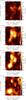 |
Fig. 5 Frames from the Faraday cube of the triplet feature at different FDs. |
There are two ubiquitous features, detected at most pixels in Ra/Dec: a peak at φ = 0 rad m-2, which is caused by the frequency-independent instrumental polarization, and a peak around φ = −12 rad m-2 (sometimes accompanied by one or two more peaks within the range −30 to 0 rad m-2). This could be polarized emission from the near side of the foreground medium of our Milky Way. Since this hampers the detection of signals from background sources or M 31 in the Faraday cube, the range ±30 rad m-2 is marked grey in all plots. An emitting foreground region is expected to be recognizable as an extended feature in the Faraday spectrum, but is not entirely visible in our observations. With a shortest wavelength of λmin ≈ 80 cm, the widest detectable feature in Faraday spectra has an extent  rad m-2. A pair of Faraday components with similar heights would indicate an extended FD structure. The quality of our data is not sufficient to rule out such structures. A large coverage in λ2 is needed to recognize components with a range of scales in the Faraday spectrum (e.g. Brentjens & de Bruyn 2005; Beck et al. 2012).
5.2.2. Comparison with previous works
Not all sources detected in the Faraday cube have been listed by Han et al. (1998) or Taylor et al. (2009) and vice versa. For the subset of sources appearing in multiple catalogues, the measured rotation measures and polarized intensities can be compared. In Fig. 6 the FD detected in our catalogue is plotted against the RM values found by Han et al. (1998; green) and Taylor et al. (2009; red). The solid line indicates where both values coincide. Although most sources agree well, several sources deviate. Here they are identified with numbers from 1 to 8, which are also given behind the names of the corresponding source in Table A.1. Sources 1 to 6 are systematically offset from the solid line towards lower absolute FDs, which suggests a systematic effect caused by Faraday depolarization.
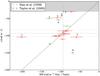 |
Fig. 6 Measured FD from the Faraday cube at 90 cm versus RM values measured by Han et al. (1998) and Taylor et al. (2009) at 20 cm. The grey area marks the range of FD that probably is affected by foreground emission and instrumental polarization. Dashed lines indicate the expected rotation measure of the Galactic foreground, dotted lines show the range spanned by the FWHM of the RMSF. |
The RM values by Han et al. (1998) and Taylor et al. (2009) were determined in the traditional way, using only two frequencies (1.365 GHz and 1.652 GHz by Han et al. 1998, 1.365 GHz and 1.435 GHz by Taylor et al. 2009). Although the frequency pairs are very close, some of their values could still be affected by the nπ ambiguity. However, this would yield an offset of ~± 650 rad m-2, which is too high to explain the offsets seen in Fig. 6. (Moreover Han et al. (1998) and Taylor et al. (2009) do not always in agree (see e.g. source 6 (37W115/T1237? or 37W045/T1126) where the PI values disagree by an order of magnitude.)
Inspection of the Faraday spectra of the sources (Figs. B.1−B.6) suggests that most of the spectra of the deviating sources have a more complex structure than those where the φ value matches the RM from previous works. The simple linear approximation of the variation of polarization angle with λ2 is only valid for the simplest case of a background source without rotation and a constant foreground screen without emission (see above). For example, the spectra of 37W074A/B (Fig. B.3, bottom right) and T1061 (Fig. B.6, top left) suggest the presence of several possibly extended RM structures along the line of sight, while the spectra of 37W175b (Fig. B.2) or 37W045/T1126 (Fig. B.4), for instance, are much more simple. Multiple components along the line of sight can easily lead to wrong results when measuring the RM between only two frequencies, which probably explains the deviations in Fig. 6.
There may also be systematic errors in the output of RM synthesis (e.g. Farnsworth et al. 2011). However, such ambiguities are within the FWHM of the RMSF. As can be seen in Fig. 6, the offset sources are well outside of this range, so they are unlikely to be caused by such systematic uncertainties resulting from RM synthesis of complicated sources.
5.2.3. Depolarization
It might be possible that the deviating sources in Fig. 6 are of a different type from those near the solid line. If these sources suffer from internal Faraday depolarization, the intrinsic FD at low frequencies can be entirely different from that at high frequencies, since the visible region of polarized emission becomes smaller (because all the emission from deeper layers is depolarized and will no longer contribute to the emission and Faraday rotation). In that case these sources should be more strongly depolarized than others. In Fig. 7 the polarization degree measured at 90 cm is plotted against that measured at 20 cm by Han et al. (1998) and Taylor et al. (2009). The deviating sources are denoted with the same numbers as given in Fig. 6. The solid grey line is a linear fit through all points; its slope corresponds the mean depolarization between 90 cm and 20 cm (DP(90,20) = 0.14 ± 0.02, χ2 = 0.76). Taking into account the large scatter, all sources (except one) follow the mean depolarization. In particular, the sources deviating in Fig. 6 are not systematically more strongly depolarized.
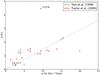 |
Fig. 7 Measured polarization degree from the Faraday cube at 90 cm versus the values measured by Han et al. (1998) and Taylor et al. (2009) at 20 cm. The solid grey line is a linear fit through all points (DP = 0.14 ± 0.02, χ2 = 0.76). |
The strong depolarization of the background sources could originate (1) in the Galactic foreground, (2) in M 31, (3) in intervening galaxies along the line of sight, or (4) in the sources themselves. The condition for model (1) is that the angular extent of the source is larger than that of a typical turbulence cell. None of our sources shows significant extension in total intensity on the scale of our telescope beam (4′), which is much smaller than the angular size of a turbulence cell in the Galactic foreground of typically 50 pc linear size out to several kiloparsecs within the Galaxy. Model (2) can be excluded because the amount of depolarization does not increase towards the inner part of M 31. We conclude that the depolarization occurs in distant intervening galaxies or within the sources.
Similarly, the multiple components seen in the Faraday spectra of Figs. B.1−B.6 can hardly originate in the Galactic foreground, because they would have to emit in polarization on similar levels as the background sources themselves (Fig. 3). They are either intrinsic features of these sources, for instance, the lobes of radio galaxies, or occur in the turbulent medium of intervening galaxies (Bernet et al. 2012). If the source is covered by a discrete number of turbulent cells in the intervenor or in the lobe, a corresponding number of components appears in the Faraday spectrum (see Fig. 5 in Bernet et al. 2012). If unresolved, these components lead to depolarization. If the number of components is large, depolarization can be described by dispersion in Faraday rotation (see Eq. (11) below).
This scenario is supported by the fact that the two sources with least depolarization (T1379 and 37W014/T1119) have simple Faraday spectra without multiple components outside the range of ±30 rad m-2, which is affected by polarized emission from the nearby foreground and by instrumental polarization. Furthermore, the three sources with the highest degrees of polarization (T1379, 37W154, and 37W019) also have simple Faraday spectra. A more detailed analysis is hampered by the small number of sources and by the fact that for most sources no data (distance, optical classification, and spectrum) are available from the literature.
37W115/T1237 is a known AGN, consisting of three components (core and two lobes, Morgan et al. 2013) that are unresolved at the resolution of our 90 cm data. It is possible that at low frequencies one of the lobes becomes depolarized, and in turn the polarized emission of the other lobe dominates (the Laing-Garrington effect, Garrington et al. 1988). In this case a comparison with 20 cm data is not practical, since one essentially observes two different source patterns. The same may also be the case for radio galaxies at larger distances.
Finally, none of our sources fits into the depolarization model for compact, steep-spectrum (CSS) sources by Rossetti et al. (2008). This model predicts that the degree of polarization should be constant at long wavelengths. The strong depolarization seen in Fig. 7 indicates that our sources are not of type CSS.
5.3. Diffuse polarized emission from M 31 and depolarization at 90 cm
No extended polarized emission of M 31 is visible by eye in the Faraday cube. Internal Faraday dispersion is the dominating depolarization mechanism towards low frequencies. Changes of the polarization angle increase with decreasing frequency. Due to turbulent cells in the magnetized plasma, the polarized emission becomes increasingly patchy and the polarization angle randomized, which is the true cause of the depolarization.
Thus it is unclear whether any coherent polarized emission on large scales can be expected at all (either in the image-plane, or in FD), therefore we propose a new method for uncovering weak diffuse polarized emission at low frequencies.
From observations at GHz frequencies it is known that the polarized emission in M 31 is strongest around the 10-kpc ring, showing an RM range of roughly −200 rad/m2 to 0 rad/m2. The intrinsic RM in M 31 is thus −100 rad/m2 to +100 rad/m2, shifted by the RM of the Galactic foreground by ~− 93 rad/m2. RM synthesis allows us to compare the positive and negative FD ranges. An excess signal in the negative FD range, which is confined to the position of M 31, would be a detection of M 31 in polarization.
We used the range of (− 100 ± 50) rad/m2 and compared it with the complementary range of (+ 100 ± 50) rad/m2. The selected range is thus centred on the FD where we expect most of the signals. Since we are in the Faraday-thick regime (opaque layer approximation, see e.g. Sokoloff et al. 1998), the total range in rotation measure will be smaller. The restriction to (− 100 ± 50) rad/m2 also excludes the range in the Faraday cube that is affected by foreground emission and instrumental polarization (see end of Sect. 5.2.1).
For each pixel in the map, we integrated along the Faraday spectrum over the absolute values in the selected positive FD range and subtracted that result from the integral along the Faraday spectrum in the selected negative FD range. Since we integrated over the amplitude of a complex-valued function, the result is by definition positive and contains a positive non-zero component from the noise. The second component in the spectrum consists of signals from M 31 itself plus a few weak, polarized point sources.
Owing to the rotation measure of the Galactic foreground, the positive FD range does not contain any significant signals of the second component. By subtracting the complementary positive FD range, we subtracted the contribution of the noise, which is equal over the entire spectrum. The residual is therefore an estimate for the intrinsic polarized signal from M 31. The positive bias from the noise component is removed with the subtraction, but due to the nonlinear addition of noise and signals in polarized intensity, weak signals are suppressed by our subtraction method, and our result is an underestimate.
Figure 8 shows the resulting residual map. Since there is still no clear detection of polarized emission, we integrated over the residual map in the image plane. After masking the detected point sources, we defined five ellipses with a width of 6′: one on the exact position where the 10-kpc ring is seen in total power (and where we expect the strongest polarization signal), one inside the ring, and three outside the ring. The outlines of the ellipses are overlaid in Fig. 8 and the results are listed in Table 1. The error in each ellipse was estimated by the standard deviation of the value in each ellipse multiplied by the sqare-root of independent resolution elements.
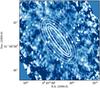 |
Fig. 8 Residual polarization map after integrating each pixel over the FD ranges (−100 ± 50) rad/m2 and (+100 ± 50) rad/m2 and subtracting the results. Overlaid are the outlines of the ellipses used to integrate in the image plane. The outline of the ellipse on the 10-kpc ring is marked in boldface. Detected point sources have been masked (seen as white points). |
Number of independent resolution elements, integrated total flux density, residual integrated polarized flux density over the selected FD range (see text) and degree of polarization.
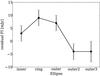 |
Fig. 9 Integrated residual polarized flux densities for the FD range ± 100 ± 50 rad m-2 for the different ellipses (see Table 1). |
We repeated the analysis for the complementary FD ranges ± 200 ± 50 rad m-2 (not shown here). As expected, no excess of polarized emission was found for these FD ranges.
Since the excess is confined to the position of polarized emission at GHz frequencies and to the expected FD range, we identified it as polarized emission originating from M 31. However, the weakness of the signals does not allow us to measure the distribution of the FD along the ring and compare this to previous results. It must be somewhat uniform or it would be visible at particular azimuthal ranges in the residual map in Fig. 8. The layer of the regular field known to exist from observations at higher frequencies is broken up by Faraday dispersion into small regions emitting in polarization. This is clearly visible in the PI map at 20 cm by Beck et al. (1998). Instead of one broad structure in the Faraday spectrum, we expect many components. Our integration collects all these features.
Now the depolarization between 6 cm and 90 cm can be estimated. The 6 cm polarized intensity map (Gießübel 2012; Gießübel et al., in prep.) was smoothed to the resolution of the 90 cm map and the total polarized flux density within the inner three ellipses was calculated (PI6 ≈ 0.296 Jy). The depolarization can then be calculated as in Beck (2007),  (9)where αn = −1.0 is the synchrotron spectral index and νi the respective frequency, leading to DP(90,6) = 0.005 ± 0.002.
The depolarization caused by internal Faraday dispersion between 20 cm and 6 cm was determined by Fletcher et al. (2004) to be DP(20,6) ≈ 0.1. Referring to Burn (1966), we can calculate the expected depolarization at 90 cm. At these low frequencies depolarization is dominated by internal Faraday dispersion. 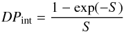 (10)with
 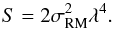 (11)The factor σRM describes the dispersion of the medium in rad m-2. In a simplified model of a magneto-ionic medium it can be written as (Arshakian & Beck 2011)
 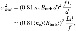 (12)where ne = ⟨ ne ⟩ /f is the thermal electron density in cm-3 within the turbulent cells of size d in pc, ⟨ ne ⟩ is the average electron density in the volume along the pathlength traced by the telescope beam in pc, f is the filling factor of the cells, ⟨ Bturb ⟩ the strength of the turbulent field in μG and L the pathlength along the line of sight through the Faraday-active emitting layer. The term in brackets describes the rotation measure of a single turbulent cell, while
  gives the number of cells along the line of sight.
The following quantities were used: ⟨ ne ⟩ = 0.015 cm-3 (in concordance with the depolarization caused by internal Faraday dispersion of 0.1, 0.3 and 0.2 measured by Fletcher et al. (2004) for different rings at 8 − 10 kpc, 10 − 12 kpc and 12 − 14 kpc, respectively), a filling factor of f = 0.2 (Walterbos & Braun 1994), Bturb = 5 μG and d = 50 pc (Fletcher et al. 2004). According to Fletcher et al. (2004), the scale height of the synchrotron-emitting layer is hsyn = 300 pc. The scale height was measured from the mid-plane. The pathlength through the entire layer along the line of sight is thus 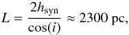 (13)where i = 75° (Chemin et al. 2009) is the inclination angle of the disk.
The classical formula by Burn (1966) would yield DP(90,6) ≈ 0.0004, p ≈ 0.03%, which essentially means total depolarization. In the model by Tribble (1991) the wavelength dependence turns from λ4 to λ2 for longer wavelengths and equation (11) becomes  (14)(see also Sokoloff et al. 1998; Arshakian & Beck 2011). This is because the dispersion causes the (spatial) correlation length of the polarized emission to decrease with increasing wavelength, until it drops below the size of the turbulent cells. In this picture, no extended structures would be visible from M 31 in the Faraday cube, which is consistent with our observations.
Since S ≫ 1, Eq. (10) becomes  (15)which (using the values given above) results in DP = 0.015, p = 1.09%.
The measured values of DP(90,6) = 0.005 ± 0.002, p = 0.21 ± 0.05% are thus between the predictions of Burn and Tribble (but closer to the latter, which is just outside our 3σ uncertainty bound). Our detection is a lower limit for the true polarized signal. If some polarized emission from M 31 is extended in Faraday space, we underestimate the detected polarized flux even more because of missing zero frequencies (see Brentjens & de Bruyn 2005). We are therefore unable to comment on the validity of the Tribble formula, but we can confidently rule out a λ4 dependence of the depolarization for low frequencies.
6. Conclusions
We have presented the first detection of polarized emission from a nearby galaxy at 90 cm. The polarized emission is mainly confined to the 10-kpc ring. At these low frequencies the emission comes from cosmic-ray electrons with lower energies. They suffer less from energy losses and therefore are able to propagate farther out from the disk or into a halo than at higher frequencies. However, no signs of a radio halo can be seen in our total power map (Fig. 1). The reason may be the preferred propagation of cosmic-ray electrons along the highly ordered field in the ring and suppression of diffusion perpendicular to the ring (Fletcher et al. 2004).
Depolarization by internal Faraday dispersion becomes strong at long wavelengths. Our observations show that the strong λ4 wavelength dependence predicted by Burn (1966) underestimates the remaining polarization at 325 MHz. We were unable to conclude whether a λ2 depolarization law as predicted by Tribble (1991) is correct, but we note that the corresponding DP does fall within our 3σ error margin. The amount of depolarization furthermore depends on the magnetic field strength, thermal electron density, and the pathlength along the line of sight and can accordingly be very different in other galaxies, depending on the conditions. A detection of diffuse polarized emission from nearby galaxies with LOFAR will be difficult and requires very high sensitivity, achievable with the RM synthesis technique in combination with a broad bandwidth. With the same parameters in Eq. (15) as used in Sect. 5.3, depolarization in the LOFAR high band around 150 MHz will be about ten times stronger. Searches for diffuse polarized emission in galaxies with LOFAR are most likely to yield detections in outer disks and halos, where σRM is expected to be much smaller than in the ring of M 31.
Using polarized background sources to probe the magnetic fields of nearby galaxies as a foreground screen seems a more promising prospect. Hence, we compiled a catalogue of all polarized point-like sources. The RM synthesis analysis resulted in 33 detections, but fewer than 50% of the sources listed by Han et al. (1998) at 20 cm were detected at 90 cm. Figure 4 shows that the number of detected sources is not sufficient to provide a grid of sources for probing the magnetic field of M 31 as a foreground screen to these sources. According to Stepanov et al. (2008), for a galaxy such as M 31, about 20 polarized sources on a cut along the projected minor axis would be needed to detect the dominant field structure (the number depends on the inclination of the galaxy, for an inclination of 45° a total number of ten would be sufficient), but the 33 sources detected here are scattered over the entire field of view. Furthermore, the estimate by Stepanov et al. (2008) assumed a constant contribution of the Milky Way foreground, which is not the case here (see Sect. 5.2.1). In conclusion, the number of polarized sources from our 90 cm observations is insufficient.
A higher angular resolution will help with the detection of more sources, since fewer features extended in RA/DEC (blending with the emission of sources) will be present in the Faraday cube. LOFAR can provide the necessary resolution, both angular and in FD.
The analysis in Sect. 5.2.2 showed that a more detailed knowledge about the structure of the sources is necessary to interpret their Faraday spectra. About 30% of the sources from the literature showed a systematically different FD at 90 cm than at 20 cm. Additional studies are needed to understand the cause of this deviation. A possible explanation is the presence of radio lobes, as discussed in Sect. 5.2.2. The systematics of the deviation (see Fig. 6 in Sect. 5.2.2) indicates that it may be possible to define distinct classes of sources and select those suitable for a background grid for future observations with LOFAR. The depolarization of the sources is on average DP(90,20) = 0.14 ± 0.02, more than seven times stronger at 90 cm than at 20 cm. If depolarization occurs due to a limited number of turbulent cells in the radio lobes or in an intervening galaxy, these cells appear as multiple components at fixed FDs in the Faraday spectrum and should be clearly resolvable with LOFAR (Beck et al. 2012). On the other hand, an emitting and Faraday-rotating region with a regular magnetic field on the line of sight, such as a radio lobe, an intervening galaxy, or a nearby region in the Milky Way, generates an extended feature in the Faraday spectrum that can be recognized at high frequencies or as a double peak at low frequencies. Future studies should combine data from GHz and MHz frequencies with RM synthesis.
Online material
Appendix A: Catalogue of detected sources
Catalogue of the detected Faraday sources.
Appendix B: Faraday spectra of the sources detected at λ90 cm
The following pages show the Faraday spectra of the sources detected at 90 cm. We refer to Sect. 5.2.1 for details. The peak associated with the detected source is marked with a blue arrow and a blue error bar. Green error bars and dashed lines show literature values from Han et al. (1998), the red errorbars and dashed lines from Taylor et al. (2009) where available.
An important selection criterion for a source to be included in the catalogue was a clear recognition as a point-like source in the cube (in RA/Dec). This is why sometimes higher peaks than the one marked as detection are present in the spectra. Any other peaks that possibly appear in the spectra are partly extended features.
The grey area marks the range of FD (± 30 rad m-2) that probably is affected by emission from the nearby foreground of the Milky Way and by instrumental polarization.
Like in Table A.1, the sources are ordered from east to west.
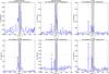 |
Fig. B.1 Faraday spectra of the detected sources. See text above for details. |
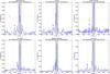 |
Fig. B.1 continued. |
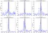 |
Fig. B.1 continued. |
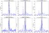 |
Fig. B.1 continued. |
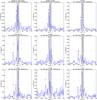 |
Fig. B.1 continued. |
For example, 752 ± 27 kpc from the luminosity of the Cepheids (Riess et al. 2012) or 744 ± 33 kpc using eclipsing binaries (Vilardell et al. 2010).
See the WSRT shadowing calculator at http://www.astron.nl/~{}heald/tools/wsrtshadow.php
Previous measurements used the radius interval R = 0−16 kpc based on the old distance estimate of 690 kpc by de Vaucouleurs & de Vaucouleurs (1964), which corresponds to R = 0−17.4 kpc using the current estimates by Riess et al. (2012) and Vilardell et al. (2010).
Acknowledgments
The authors would like to thank Björn Adebahr and Carlos Sotomayor (Ruhr-Universität Bochum) for their initial help with calibration and peeling in CASA, and Elly M. Berkhuijsen for valuable comments. We are also grateful for the comments of the anonymous referee, which helped to improve our paper. R.B. acknowledges support from DFG FOR1254. T.G.A. acknowledges support by DFG project number Os 177/2-1. The presented results and images have in part been published in Gießübel (2012). The Westerbork Synthesis Radio Telescope is operated by the ASTRON (Netherlands Institute for Radio Astronomy) with support from the Netherlands Foundation for Scientific Research (NWO).
References
- Arshakian, T. G., & Beck, R. 2011, MNRAS, 418, 2336 [NASA ADS] [CrossRef] [Google Scholar]
- Beck, R. 1982, A&A, 106, 121 [NASA ADS] [Google Scholar]
- Beck, R. 2005, in Magnetic Fields in the Universe: From Laboratory and Stars to Primordial Structures, eds. E. M. de Gouveia dal Pino, G. Lugones, & A. Lazarian, AIP Conf. Ser., 784, 343 [Google Scholar]
- Beck, R. 2007, A&A, 470, 539 [NASA ADS] [CrossRef] [EDP Sciences] [Google Scholar]
- Beck, R., Berkhuijsen, E. M., & Wielebinski, R. 1978, A&A, 68, L27 [NASA ADS] [Google Scholar]
- Beck, R., Brandenburg, A., Moss, D., Shukurov, A., & Sokoloff, D. 1996, ARA&A, 34, 155 [NASA ADS] [CrossRef] [Google Scholar]
- Beck, R., Berkhuijsen, E. M., & Hoernes, P. 1998, A&AS, 129, 329 [NASA ADS] [CrossRef] [EDP Sciences] [Google Scholar]
- Beck, R., Frick, P., Stepanov, R., & Sokoloff, D. 2012, A&A, 543, A113 [NASA ADS] [CrossRef] [EDP Sciences] [Google Scholar]
- Berkhuijsen, E. M., Beck, R., & Hoernes, P. 2003, A&A, 398, 937 [NASA ADS] [CrossRef] [EDP Sciences] [Google Scholar]
- Bernet, M. L., Miniati, F., & Lilly, S. J. 2012, ApJ, 761, 144 [NASA ADS] [CrossRef] [Google Scholar]
- Brentjens, M. A. 2008, A&A, 489, 69 [NASA ADS] [CrossRef] [EDP Sciences] [Google Scholar]
- Brentjens, M. A., & de Bruyn, A. G. 2005, A&A, 441, 1217 [NASA ADS] [CrossRef] [EDP Sciences] [Google Scholar]
- Burn, B. J. 1966, MNRAS, 133, 67 [NASA ADS] [CrossRef] [Google Scholar]
- Chemin, L., Carignan, C., & Foster, T. 2009, ApJ, 705, 1395 [NASA ADS] [CrossRef] [Google Scholar]
- Cornwell, T. J., Holdaway, M. A., & Uson, J. M. 1993, A&A, 271, 697 [NASA ADS] [Google Scholar]
- de Vaucouleurs, G., & de Vaucouleurs, A. 1964, Ref. Catalogue of Bright Galaxies (Austin: Univ. of Texas Press) [Google Scholar]
- Farnsworth, D., Rudnick, L., & Brown, S. 2011, AJ, 141, 191 [NASA ADS] [CrossRef] [Google Scholar]
- Fletcher, A. 2010, in ASP Conf. Ser. 438, eds. R. Kothes, T. L. Landecker, & A. G. Willis, 197 [Google Scholar]
- Fletcher, A., Berkhuijsen, E. M., Beck, R., & Shukurov, A. 2004, A&A, 414, 53 [NASA ADS] [CrossRef] [EDP Sciences] [Google Scholar]
- Fomalont, E. B. 1999, in Synthesis Imaging in Radio Astronomy II, eds. G. B. Taylor, C. L. Carilli, & R. A. Perley, ASP Conf. Ser., 180, 301 [Google Scholar]
- Garrington, S. T., Leahy, J. P., Conway, R. G., & Laing, R. A. 1988, Nature, 331, 147 [NASA ADS] [CrossRef] [Google Scholar]
- Gießübel, R. 2012, Ph.D. Dissertation, Universität zu Köln, Cuvillier Verlag Göttingen [Google Scholar]
- Gräve, R., Emerson, D. T., & Wielebinski, R. 1981, A&A, 98, 260 [NASA ADS] [Google Scholar]
- Hamaker, J. P., Bregman, J. D., & Sault, R. J. 1996, A&AS, 117, 137 [NASA ADS] [CrossRef] [EDP Sciences] [Google Scholar]
- Han, J. L., Beck, R., & Berkhuijsen, E. M. 1998, A&A, 335, 1117 [NASA ADS] [Google Scholar]
- Heald, G. 2009, in IAU Symp., 259, 591 [Google Scholar]
- Heald, G., Braun, R., & Edmonds, R. 2009, A&A, 503, 409 [NASA ADS] [CrossRef] [EDP Sciences] [Google Scholar]
- Morgan, J. S., Argo, M. K., Trott, C. M., et al. 2013, ApJ, 768, 12 [NASA ADS] [CrossRef] [Google Scholar]
- Offringa, A. R., de Bruyn, A. G., Biehl, M., et al. 2010, MNRAS, 405, 155 [NASA ADS] [Google Scholar]
- Perley, R. A., & Taylor, G. B. 2003, http://www.vla.nrao.edu/astro/calib/manual/calman.ps.gz [Google Scholar]
- Popping, A., & Braun, R. 2008, A&A, 479, 903 [NASA ADS] [CrossRef] [EDP Sciences] [Google Scholar]
- Riess, A. G., Fliri, J., & Valls-Gabaud, D. 2012, ApJ, 745, 156 [NASA ADS] [CrossRef] [Google Scholar]
- Rossetti, A., Dallacasa, D., Fanti, C., Fanti, R., & Mack, K.-H. 2008, A&A, 487, 865 [NASA ADS] [CrossRef] [EDP Sciences] [Google Scholar]
- Sault, R. J., Teuben, P. J., & Wright, M. C. H. 1995, in Astronomical Data Analysis Software and Systems IV, eds. R. A. Shaw, H. E. Payne, & J. J. E. Hayes, ASP Conf. Ser., 77, 433 [Google Scholar]
- Sault, R. J., Staveley-Smith, L., & Brouw, W. N. 1996, A&AS, 120, 375 [NASA ADS] [CrossRef] [EDP Sciences] [Google Scholar]
- Scaife, A. M. M., & Heald, G. H. 2012, MNRAS, L434 [Google Scholar]
- Simard-Normandin, M., Kronberg, P. P., & Button, S. 1981, ApJS, 45, 97 [NASA ADS] [CrossRef] [Google Scholar]
- Sokoloff, D. D., Bykov, A. A., Shukurov, A., et al. 1998, MNRAS, 299, 189 [NASA ADS] [CrossRef] [Google Scholar]
- Stepanov, R., Arshakian, T. G., Beck, R., Frick, P., & Krause, M. 2008, A&A, 480, 45 [NASA ADS] [CrossRef] [EDP Sciences] [Google Scholar]
- Taylor, A. R., Stil, J. M., & Sunstrum, C. 2009, ApJ, 702, 1230 [NASA ADS] [CrossRef] [Google Scholar]
- Tribble, P. C. 1991, MNRAS, 250, 726 [NASA ADS] [CrossRef] [Google Scholar]
- van Haarlem, M. P., Wise, M. W., Gunst, A. W., et al. 2013, A&A, 556, A2 [NASA ADS] [CrossRef] [EDP Sciences] [Google Scholar]
- Vilardell, F., Ribas, I., Jordi, C., Fitzpatrick, E. L., & Guinan, E. F. 2010, A&A, 509, A70 [NASA ADS] [CrossRef] [EDP Sciences] [Google Scholar]
- Walterbos, R. A. M., & Braun, R. 1994, ApJ, 431, 156 [NASA ADS] [CrossRef] [Google Scholar]
- Walterbos, R. A. M., Brinks, E., & Shane, W. W. 1985, A&AS, 61, 451 [NASA ADS] [Google Scholar]
All Tables
Number of independent resolution elements, integrated total flux density, residual integrated polarized flux density over the selected FD range (see text) and degree of polarization.
All Figures
|
Fig. 1 Final total power image of M 31 at 90 cm. Contours are from 4 to 128 mJy/beam in steps of 10 mJy/beam. HPBW: 230′′ × 290′′; rms = 1.4 mJy/beam. The black crosses mark the pointing centres of the two fields. Note: the tick marks may be misleading since the map is rotated with respect to the celestial coordinates, see the coordinate grid in Fig. 2 or Fig. 4. |
| In the text | |
|
Fig. 2 Spectral index (SI) map between 90 cm and 20 cm overlaid with the same contours as Fig. 1. The SI map was calculated for intensities >5σ in Stokes I. |
| In the text | |
|
Fig. 3 Example for a set of different polarization-emitting and rotating components along the line of sight and the resulting Faraday spectrum. E1 and E3 are point sources, E2,R2 is an extended emitting and rotating region. R1, R3, and R4 are Faraday screens that are not emitting. Depolarization effects are neglected here for simplicity. |
| In the text | |
|
Fig. 4 Position and Faraday depth of the detected sources on contours of the total power map. |
| In the text | |
|
Fig. 5 Frames from the Faraday cube of the triplet feature at different FDs. |
| In the text | |
|
Fig. 6 Measured FD from the Faraday cube at 90 cm versus RM values measured by Han et al. (1998) and Taylor et al. (2009) at 20 cm. The grey area marks the range of FD that probably is affected by foreground emission and instrumental polarization. Dashed lines indicate the expected rotation measure of the Galactic foreground, dotted lines show the range spanned by the FWHM of the RMSF. |
| In the text | |
|
Fig. 7 Measured polarization degree from the Faraday cube at 90 cm versus the values measured by Han et al. (1998) and Taylor et al. (2009) at 20 cm. The solid grey line is a linear fit through all points (DP = 0.14 ± 0.02, χ2 = 0.76). |
| In the text | |
|
Fig. 8 Residual polarization map after integrating each pixel over the FD ranges (−100 ± 50) rad/m2 and (+100 ± 50) rad/m2 and subtracting the results. Overlaid are the outlines of the ellipses used to integrate in the image plane. The outline of the ellipse on the 10-kpc ring is marked in boldface. Detected point sources have been masked (seen as white points). |
| In the text | |
|
Fig. 9 Integrated residual polarized flux densities for the FD range ± 100 ± 50 rad m-2 for the different ellipses (see Table 1). |
| In the text | |
|
Fig. B.1 Faraday spectra of the detected sources. See text above for details. |
| In the text | |
|
Fig. B.1 continued. |
| In the text | |
|
Fig. B.1 continued. |
| In the text | |
|
Fig. B.1 continued. |
| In the text | |
|
Fig. B.1 continued. |
| In the text | |
Current usage metrics show cumulative count of Article Views (full-text article views including HTML views, PDF and ePub downloads, according to the available data) and Abstracts Views on Vision4Press platform.
Data correspond to usage on the plateform after 2015. The current usage metrics is available 48-96 hours after online publication and is updated daily on week days.
Initial download of the metrics may take a while.