| Issue |
A&A
Volume 558, October 2013
|
|
|---|---|---|
| Article Number | A144 | |
| Number of page(s) | 9 | |
| Section | Extragalactic astronomy | |
| DOI | https://doi.org/10.1051/0004-6361/201322203 | |
| Published online | 23 October 2013 | |
Causal connection in parsec-scale relativistic jets: results from the MOJAVE VLBI survey
1
Max-Planck-Institut für Radioastronomie,
Auf dem Hügel 69,
53121
Bonn,
Germany
e-mail:
This email address is being protected from spambots. You need JavaScript enabled to view it.
2
Crimean Astrophysical Observatory, 98409
Nauchny, Crimea,
Ukraine
3
Pulkovo Astronomical Observatory, Pulkovskoe Chaussee 65/1, 196140
St. Petersburg,
Russia
4
Astro Space Center of Lebedev Physical Institute,
Profsoyuznaya
84/32, 117997
Moscow,
Russia
Received:
3
July
2013
Accepted:
8
September
2013
Abstract
We report that active galactic nucleus (AGN) jets are causally connected on parsec scales, based on 15 GHz Very Long Baseline Array (VLBA) data from a sample of 133 AGN jets. This result is achieved through a new method for measuring the product of the jet Lorentz factor and the intrinsic opening angle Γθj from measured apparent opening angles in flux density limited samples of AGN jets. The Γθj parameter is important for jet physics because it is related to the jet-frame sidewise expansion speed and causal connection between the jet edges and its symmetry axis. Most importantly, the standard model of jet production requires that the jet be causally connected with its symmetry axis, implying that Γθj ≲ 1. When we apply our method to the MOJAVE flux density limited sample of radio loud objects, we find Γθj ≈ 0.2, implying that AGN jets are causally connected. We also find evidence that AGN jets viewed very close to the line of sight effectively have smaller intrinsic opening angles compared with jets viewed more off-axis, which is consistent with Doppler beaming and a fast inner spine/slow outer sheath velocity field. Notably, gamma-ray burst (GRB) jets have a typical Γθj that is two orders of magnitude higher, suggesting that different physical mechanisms are at work in GRB jets compared to AGN jets. A useful application of our result is that a jet’s beaming parameters can be derived. Assuming Γθj is approximately constant in the AGN jet population, an individual jet’s Doppler factor and Lorentz factor (and therefore also its viewing angle) can be determined using two observable quantities: apparent jet opening angle and the apparent speed of jet components.
Key words: galaxies: active / quasars: general / galaxies: jets / BL Lacertae objects: general / gamma-ray burst: general
© ESO, 2013
1. Introduction
A wide variety of processes in relativistic outflows are sensitive to causal connection, or the ability of a disturbance at the edge of an axisymmetric flow to communicate with the symmetry axis1. In the standard magnetic model of relativistic jet production (Beskin 2010), the global jet structure determines the nature of bulk acceleration, implying that the jet must be causally connected for such acceleration to take place (e.g., Tchekhovskoy et al. 2009; Komissarov et al. 2009). Causal connection is determined by the half opening angle of an axisymmetric flow, θj, and the flow Lorentz factor, Γ, through their product Γθj, where Γθj ≲ 1 implies that the jet is causally connected. Other important aspects of relativistic jet physics that depend on Γθj include jet stability (Narayan et al. 2009), magnetic reconnection (Giannios 2013), recollimation shock energy dissipation (Nalewajko & Sikora 2009), and recollimation shock structure (Kohler et al. 2012).
Relativistic outflows have a wide range of values of Γθj. On the one hand, pulsar wind nebulae contain uncollimated (equitorial) outflows that are inferred to reach very high bulk Lorentz factors of Γ ~ 106 prior to the termination shock (Kennel & Coroniti 1984), implying that these outflows have values of Γθj ~ 106 and are not causally connected. On the other hand, narrow relativistic outflows (i.e., jets) associated with X-ray binaries (XRBs), gamma-ray bursts (GRBs), and active galactic nucleus (AGN) typically have much lower values of Γθj; GRB light curve analyses lead to typical inferred values of Γθj of 10−30 (Panaitescu & Kumar 2002), while the narrowness and moderate apparent speeds in XRB jets support the assumption that Γθj ≲ 1 (e.g., Miller-Jones et al. 2006). Thus, while the central engines of the abovementioned objects are similar in that they involve compact magnetized spinning objects, their different values of Γθj suggest that different physical processes are at work.
There have been two past measurements of the characteristic value of Γθj for AGN jets. Using 7 mm Very Long Baseline Array (VLBA) data from 15 different AGN jets, Jorstad et al. (2005) measured Γθj by assuming that the observed pattern speed of moving jet components corresponds to the jet bulk flow speed, and that the component variability times are equal to the jet frame light crossing times of the resolved components. From these assumptions they determined the component’s Lorentz factor and jet half-opening angle, and found an anti-correlation between the derived values of θj and Γ, with Γθj = 0.17. With a larger sample of 56 AGN jets from 15 GHz VLBA data, Pushkarev et al. (2009) performed the same analysis, except they used jet parameters from Hovatta et al. (2009), who derived these values from variability time, maximum flux density of flares, and equipartition derived brightness temperature arguments. The Pushkarev et al. (2009) analysis found a similar anti-correlation with Γθj = 0.13.
Motivated by the above theoretical concerns, we construct a very different method of inferring Γθj by using apparent opening angles obtained from a flux density limited sample of AGN jets. We construct a theoretical probability density function for apparent opening angles in a flux density limited sample, which we derive in Sect. 2, and which has Γθj as a free parameter to be fixed by finding the best fit to an empirical distribution of apparent opening angles. Our data consist of the stacked images from 135 AGN jets that make up the MOJAVE-I sample, a 15 GHz flux density limited survey conducted by the VLBA of radio sources in the northern sky with flux densities above 1.5 Jy, and above 2 Jy for sources with − 20 < dec < 0 (Lister et al. 2009a). The stacked images and opening angles are also discussed and analyzed in Pushkarev et al. (2012). After analyzing the data in Sect. 3, we discuss in Sect. 4 the physical significance of the parameter Γθj for AGN in the context of jet instabilities, GRB jet acceleration vs. AGN jet acceleration, and jet parameter estimation. We conclude in Sect. 5.
2. Statistical model of θapp
Here we model a given jet’s value of θapp as a random variable that is drawn from the probability density function (PDF) P(θapp). That is, P(θapp)dθapp represents the probability that a given jet in a flux density limited sample will have an observed apparent half opening angle between θapp and θapp + dθapp. First, however, we motivate our model by estimating Γθj for blazars, and discuss the effect that velocity shear may have on jet appearance.
Blazars are oriented such that the angle between the jet symmetry axis and the line sight,
θob, is x/Γ, where
x ≈ 0.5 on average in flux density limited samples (Vermeulen & Cohen 1994) such as MOJAVE. This value for
x implies an upper limit on Γθj of
 This
is based on the simple argument that most MOJAVE jets are not observed “down the pipe”,
(= θob < θj),
since a down-the-pipe AGN jet would not display jet-like morphology. In fact, most MOJAVE
sources do display a jet-like morphology, which implies that typically
θob > θj
(Clausen-Brown et al. 2011), and therefore that
0.5/Γ > θj
according to the typical value of θob for flux density limited
samples. Also, an estimate of Γθj can be made,
This
is based on the simple argument that most MOJAVE jets are not observed “down the pipe”,
(= θob < θj),
since a down-the-pipe AGN jet would not display jet-like morphology. In fact, most MOJAVE
sources do display a jet-like morphology, which implies that typically
θob > θj
(Clausen-Brown et al. 2011), and therefore that
0.5/Γ > θj
according to the typical value of θob for flux density limited
samples. Also, an estimate of Γθj can be made,  (1)where
⟨ θapp ⟩ ≈ 0.2 rad is the average apparent opening angle in
the MOJAVE-I sample that we use in this work. From geometrical considerations, as long as
all the relevant angles are small,
θj = θobθapp,
thus if ⟨ θapp ⟩ is used for θapp
and 0.5/Γ for θob, then we obtain Eq. (1). An interesting feature of the above estimate
is that it does not significantly depend on the actual value of Γ, which is useful since
jets possess a wide range of Γ values (Lister et al.
2009b). In Sect. 2.1 we will make a more
rigorous analysis of the likely value of Γθj for blazars in
which we will also find that this estimate is mostly independent of blazar values of Γ.
(1)where
⟨ θapp ⟩ ≈ 0.2 rad is the average apparent opening angle in
the MOJAVE-I sample that we use in this work. From geometrical considerations, as long as
all the relevant angles are small,
θj = θobθapp,
thus if ⟨ θapp ⟩ is used for θapp
and 0.5/Γ for θob, then we obtain Eq. (1). An interesting feature of the above estimate
is that it does not significantly depend on the actual value of Γ, which is useful since
jets possess a wide range of Γ values (Lister et al.
2009b). In Sect. 2.1 we will make a more
rigorous analysis of the likely value of Γθj for blazars in
which we will also find that this estimate is mostly independent of blazar values of Γ.
A possibility we explore below is that there is a viewing angle effect related to Doppler beaming and velocity shear that affects the appearance of blazars. Velocity shear is included in a variety of AGN jet models, including parsec-scale models (Swain & Bridle 1998; Attridge et al. 1999; Tavecchio & Ghisellini 2008; Perucho et al. 2012), kiloparsec-scale models (e.g. Owen et al. 1989; Swain & Bridle 1998; Perlman et al. 1999; Laing & Bridle 2004), and more general jet models (Aloy et al. 2000; Chiaberge et al. 2000; McKinney 2006). We assume velocity shear affects very long baseline interferometry (VLBI) measurements of a jet’s apparent opening angle θapp. While all jets may have the same value of Γθj, for jets viewed with very small viewing angles the emission might originate from a fast (beamed) narrow spine that is a fraction of the true jet opening angle θj, while for jets with larger viewing angles the emission from a slow outer sheath with half-opening angle θj may be more detectable. This effect is described in Sect. 2.2.
2.1. Derivation of P(θapp)
To test the viability of the simplest case scenario, we assume that
Γθj is constant for all relativistic jets, and that these
jets are conical and non-accelerating. In general, however, jets are not conical and the
jet flow is either accelerating or decelerating, although in some jet models
Γθj nevertheless remains constant (e.g., Zakamska et al. 2008). Individual observed jet
component acceleration is consistent with only very small changes in Lorentz factor,
 (Homan et al. 2009), although an individual jet
does posses a range of component speeds (Lister et al.
2009b, 2013). Thus, our assumption of
conical non-accelerating jets clearly introduces uncertainty to our model.
(Homan et al. 2009), although an individual jet
does posses a range of component speeds (Lister et al.
2009b, 2013). Thus, our assumption of
conical non-accelerating jets clearly introduces uncertainty to our model.
As we show below, Γθj is a free parameter of
P(θapp), and thus will be determined in the
fit to the empirical distribution of θapp. To derive
P(θapp), we first derive the PDF for
viewing angles, P(θob). If the sample of AGN
jets is unbiased with respect to orientation,
P(θob) = sinθob.
However, because it is flux density limited, it will take the form
 This
additional factor takes into account that more sources are directed at the observer in a
flux density limited sample because Doppler beamed jets are detectable at greater
distances than unbeamed ones. Cohen (1989) and Vermeulen & Cohen (1994) computed this term and
found that it depends on the bulk Lorentz factor distribution in a flux density limited
sample, the integral source count index, and the beaming index of the jet. The beaming
index is defined from the relation
F = δnF′,
where n is the beaming index, δ is the Doppler factor,
F is the observed flux density density, and
F′ is the intrinsic flux density. The observed integral
source count index is defined in the expression
N(>F) ∝ F− q,
representing the number of sources N observed with a flux density above
F, which is a power law in F with source count index
q. Including the Doppler bias factor in the viewing angle PDF gives
This
additional factor takes into account that more sources are directed at the observer in a
flux density limited sample because Doppler beamed jets are detectable at greater
distances than unbeamed ones. Cohen (1989) and Vermeulen & Cohen (1994) computed this term and
found that it depends on the bulk Lorentz factor distribution in a flux density limited
sample, the integral source count index, and the beaming index of the jet. The beaming
index is defined from the relation
F = δnF′,
where n is the beaming index, δ is the Doppler factor,
F is the observed flux density density, and
F′ is the intrinsic flux density. The observed integral
source count index is defined in the expression
N(>F) ∝ F− q,
representing the number of sources N observed with a flux density above
F, which is a power law in F with source count index
q. Including the Doppler bias factor in the viewing angle PDF gives
 (2)where
a = nq − 1, P(Γ) is the PDF for jet
bulk Lorentz factor, and A is the normalization constant. An important
assumption made in calculating the Doppler bias term is that the log-log slope of
N(>F′) vs.
F′ and
N(>F) vs. F
are the same, which Vermeulen & Cohen
(1994) justify based on previous studies of AGN jet luminosity functions (Urry & Shafer 1984; Urry & Padovani 1991). The MOJAVE selection criteria were
designed so that source inclusion in the sample is based on beamed emission only (Lister & Homan 2005). These MOJAVE sources are
typically dominated by core flux density, which usually has a flat spectrum (Kovalev et al. 2005; Pushkarev & Kovalev 2012). Thus, the beaming index n is
most likely ~2 for steady jets (Lind & Blandford
1985), while the integral source count index is approximately 1.5, indicating
that the fiducial value for the a-parameter should be approximately
(Vermeulen & Cohen 1994)
(2)where
a = nq − 1, P(Γ) is the PDF for jet
bulk Lorentz factor, and A is the normalization constant. An important
assumption made in calculating the Doppler bias term is that the log-log slope of
N(>F′) vs.
F′ and
N(>F) vs. F
are the same, which Vermeulen & Cohen
(1994) justify based on previous studies of AGN jet luminosity functions (Urry & Shafer 1984; Urry & Padovani 1991). The MOJAVE selection criteria were
designed so that source inclusion in the sample is based on beamed emission only (Lister & Homan 2005). These MOJAVE sources are
typically dominated by core flux density, which usually has a flat spectrum (Kovalev et al. 2005; Pushkarev & Kovalev 2012). Thus, the beaming index n is
most likely ~2 for steady jets (Lind & Blandford
1985), while the integral source count index is approximately 1.5, indicating
that the fiducial value for the a-parameter should be approximately
(Vermeulen & Cohen 1994)
 We
note that if the MOJAVE sources were typically dominated by optically thin flux density,
which typically has a spectral index of α ~ 0.7
(Fν ∝ ν− α),
then a ≈ 3.
We
note that if the MOJAVE sources were typically dominated by optically thin flux density,
which typically has a spectral index of α ~ 0.7
(Fν ∝ ν− α),
then a ≈ 3.
The opening angle distribution may now be derived from
P(θob,Γ) by a change of
variables from θob to θapp and
marginalizing over Γ,  (3)where
θob and
∂θob/∂θapp
are functions of θapp and Γ, and can be determined by assuming
a particular jet geometry that we take to be conical here. These relationships are often
derived by treating conical jets as triangles projected onto the plane of the sky,
implying that
tanθapp = Rj/ℓ′ = Rj/(ℓsinθob),
where θob is the jet viewing angle,
Rj is the jet radius, ℓ
is the jet length, and ℓ′ is the jet length projected onto the
sky. If we assume
θj ≈ Rj/ℓ,
then
(3)where
θob and
∂θob/∂θapp
are functions of θapp and Γ, and can be determined by assuming
a particular jet geometry that we take to be conical here. These relationships are often
derived by treating conical jets as triangles projected onto the plane of the sky,
implying that
tanθapp = Rj/ℓ′ = Rj/(ℓsinθob),
where θob is the jet viewing angle,
Rj is the jet radius, ℓ
is the jet length, and ℓ′ is the jet length projected onto the
sky. If we assume
θj ≈ Rj/ℓ,
then  (4)For
cases where both θapp and θj are
≪1, this reduces to a commonly used relation for jets,
θj = θappsinθob
(Jorstad et al. 2005; Pushkarev et al. 2009). Equation (4) also implies a maximum apparent half-opening angle of
π/2. We assume that jets viewed down-the-pipe where
θob < θj
are rare, since such jets would have
θapp > π/2.
This dearth of down-the-pipe jets, sometimes used to justify the cylindrical approximation
in jet models (Clausen-Brown et al. 2011), also
indicates that typically Γθj < 1. If
the typical viewing angle of a jet is
θob = 0.5/Γ (Vermeulen & Cohen 1994), and most MOJAVE jets exhibit a
jet-like morphology (i.e.,
θapp < π/2)
such that
θob > θj,
then Γθj < 0.5. Here, because many
jets have large apparent opening angles, but are often viewed with small observing angles
and small intrinsic opening angles, we most often use the approximation that
(4)For
cases where both θapp and θj are
≪1, this reduces to a commonly used relation for jets,
θj = θappsinθob
(Jorstad et al. 2005; Pushkarev et al. 2009). Equation (4) also implies a maximum apparent half-opening angle of
π/2. We assume that jets viewed down-the-pipe where
θob < θj
are rare, since such jets would have
θapp > π/2.
This dearth of down-the-pipe jets, sometimes used to justify the cylindrical approximation
in jet models (Clausen-Brown et al. 2011), also
indicates that typically Γθj < 1. If
the typical viewing angle of a jet is
θob = 0.5/Γ (Vermeulen & Cohen 1994), and most MOJAVE jets exhibit a
jet-like morphology (i.e.,
θapp < π/2)
such that
θob > θj,
then Γθj < 0.5. Here, because many
jets have large apparent opening angles, but are often viewed with small observing angles
and small intrinsic opening angles, we most often use the approximation that  (5)This
approximation is mostly appropriate for the blazar dominated MOJAVE sample; below in
Sect. 2.2 we show that this approximation is useful
for categorizing jets by their apparent opening angles.
(5)This
approximation is mostly appropriate for the blazar dominated MOJAVE sample; below in
Sect. 2.2 we show that this approximation is useful
for categorizing jets by their apparent opening angles.
An apparent weakness in our model is that P(Γ) is not well constrained.
This is not the case, however, since P(θapp)
is insensitive to P(Γ), which we demonstrate here. In a flux density
limited VLBI sample, jets with small viewing angles will dominate, so we assume
sinθob ≈ θob, and approximate
(2) as  (6)For
simplicity, we now evaluate Eq. (3) in
light of the geometry implied by Eq. (5),
and obtain
(6)For
simplicity, we now evaluate Eq. (3) in
light of the geometry implied by Eq. (5),
and obtain ![Mathematical equation: \begin{eqnarray} P(\tapp)&=A\left(1+\frac{\rho^2}{\tan^2{\tapp}}\right)^{-a-1}\frac{\cos{\tapp}}{\sin^3{\tapp}} \notag\\ &\quad \times\left[2^{a\,+\,1}\rho^2\int{\Gamma^{2a}P(\Gamma){\rm d}\Gamma}\right] \notag\\ &= A'\left(1+\frac{\rho^2}{\tan^2{\tapp}}\right)^{-a-1}\frac{\cos{\tapp}}{\sin^3{\tapp}}, \label{approx2} \end{eqnarray}](/articles/aa/full_html/2013/10/aa22203-13/aa22203-13-eq83.png) (7)where
ρ = Γθj, and we have absorbed the term in
brackets into the new normalization, A′. Thus, it is apparent
from Eq. (7) that
P(θapp) does not depend significantly on
the form of P(Γ). Equation (7) is an accurate approximation of
P(θapp) as long as ρ ≪ 1,
which is a valid assumption as shown by our best value of ρ ≈ 0.2
discussed below.
(7)where
ρ = Γθj, and we have absorbed the term in
brackets into the new normalization, A′. Thus, it is apparent
from Eq. (7) that
P(θapp) does not depend significantly on
the form of P(Γ). Equation (7) is an accurate approximation of
P(θapp) as long as ρ ≪ 1,
which is a valid assumption as shown by our best value of ρ ≈ 0.2
discussed below.
2.2. Velocity shear and Doppler beaming
As suggested by the very approximate estimate made above in which radio galaxies appear to have larger θj than blazars, velocity shear and Doppler beaming may affect the distribution of θapp. Unfortunately, modeling the effect of velocity of shear on jet appearance is sensitive to a variety of unknown details regarding the jet structure such as how the density of non-thermal electrons scales with jet radius and the particular functional form of the velocity shear. Thus, in an effort to capture only the most basic effect velocity shear has on jet appearance, we develop a minimalist model.
We assume the velocity field of a jet consists of an ultra-relativistic inner spine and a surrounding shear layer that is mildly relativistic (see Fig. 2). The relativistic spine, which dominates the core emission, is what primarily determines whether a jet is included in a flux density limited sample like the blazar dominated MOJAVE sample. We note, however, that this assumption may sometimes be violated since a few MOJAVE sources such as M87 may have significant sheath emission (e.g., Kovalev et al. 2007). The optically thin jet downstream from the core is where apparent opening angles are measured, and where the degree to which the shear layer is observable is important. For jets aligned close to the line of sight, the jets will be more dominated by the fast spine where Γ ≫ 1 and the slower outer layers will remain unobserved, while more misaligned the jets will have a slower outer sheath of Γshear≲ few that is more likely visible. See Fig. 1 for an illustration of this effect.
Now, jets can be divided into two categories based on whether a jet’s viewing angle
θob is less than or greater than 1/Γ,
where Γ is the value of the Lorentz factor in the fast inner spine. This categorization
can be mapped onto θapp by using Eq. (5), resulting in
 (8)This
categorization is useful since the critical angle 1/Γ defines when
beaming is important. When
θob > 1/Γ, then
Earth is outside of the inner jet’s beaming cone, thus the jet’s slower outer layers are
more likely to be visible, since the fast inner spine’s beaming is less dominant. The
hypothesis that highly beamed jets
(θob < 1/Γ) and
not highly beamed jets
(θob > 1/Γ) can
be separated by their observed θapp has some observational
support, which we discuss in Sect. 4.3.
(8)This
categorization is useful since the critical angle 1/Γ defines when
beaming is important. When
θob > 1/Γ, then
Earth is outside of the inner jet’s beaming cone, thus the jet’s slower outer layers are
more likely to be visible, since the fast inner spine’s beaming is less dominant. The
hypothesis that highly beamed jets
(θob < 1/Γ) and
not highly beamed jets
(θob > 1/Γ) can
be separated by their observed θapp has some observational
support, which we discuss in Sect. 4.3.
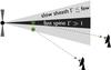 |
Fig. 1 Meridional slice of a jet illustrating two cases: (i) jets aligned close to the line of sight where emission is dominated by the fast inner spine; and (ii) more misaligned jets where the emission from outer slower layers contributes as well. |
The simplest way to model the effect that velocity shear and beaming have on jet
appearence is to postulate that jets that have
θob < 1/Γ have an
effective jet opening angle
θj,eff = ρeff/Γ,
where θj,eff is some fraction of the true jet
opening angle such that
θj,eff = fshθj,
or equivalenty,
ρeff = fshρ.
Thus, 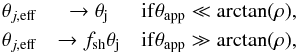 where
fsh is a free parameter. We note that the inner spine
Doppler factor of a jet with
θapp ~ θj (i.e., a radio galaxy)
is δ ~ 1/Γ, a jet with
θapp = ρ has δ ~ Γ, and a
jet with θapp ~ 1 has δ ~ 2Γ. In other words,
the most drastic change in δ occurs in a narrow range of
θapp, for
0 < θapp < ρ,
while δ only changes by a factor of 2 in the large range
ρ < θapp ≲ 1. To
illustrate this point, we plot the Doppler factor as a function of
θapp in Fig. 2. Thus,
the effect of velocity shear on jet appearance should be strongest for
θapp = 0 to ρ. To reproduce this behavior,
we choose the following arbitrary function,
where
fsh is a free parameter. We note that the inner spine
Doppler factor of a jet with
θapp ~ θj (i.e., a radio galaxy)
is δ ~ 1/Γ, a jet with
θapp = ρ has δ ~ Γ, and a
jet with θapp ~ 1 has δ ~ 2Γ. In other words,
the most drastic change in δ occurs in a narrow range of
θapp, for
0 < θapp < ρ,
while δ only changes by a factor of 2 in the large range
ρ < θapp ≲ 1. To
illustrate this point, we plot the Doppler factor as a function of
θapp in Fig. 2. Thus,
the effect of velocity shear on jet appearance should be strongest for
θapp = 0 to ρ. To reproduce this behavior,
we choose the following arbitrary function,  (9)We
plot this function in Fig. 2. This equation can
easily be inserted into our theoretical PDF described in Eq. (3), which can then be evaluated numerically,
where ρ and fsh are free parameters to be
found in the fit. If this model is correct, then the best fit value of
fsh should be less than unity. In the case of no shear, then
fsh = 1 and
ρeff = ρ.
(9)We
plot this function in Fig. 2. This equation can
easily be inserted into our theoretical PDF described in Eq. (3), which can then be evaluated numerically,
where ρ and fsh are free parameters to be
found in the fit. If this model is correct, then the best fit value of
fsh should be less than unity. In the case of no shear, then
fsh = 1 and
ρeff = ρ.
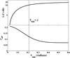 |
Fig. 2 Doppler factor and ρeff as a function of a jet’s apparent half-opening angle θapp. The semi-logarithmic Doppler factor plot in the upper panel is for a jet with Γ = 10 and ρ = 0.21, and uses Eq. (4) to convert θapp to θob. The lower panel plot shows ρeff as a function of θapp from Eq. (9) using ρ = 0.21 and fsh = 0.33, the best fit values found in Sect. 3.2. |
3. Data analysis and results
3.1. Apparent opening angles
The apparent opening angles used here are derived from stacked images of 133 sources from
the MOJAVE-I catalogue of 135 sources2. For two
sources opening angles could not be derived. To produce a stacked image of a given source,
all single-epoch maps were aligned by their VLBI core components, and then averaged
together. The resulting opening angle data originates from the analysis in Pushkarev et al. (2012), who derived
θapp by taking the median value of
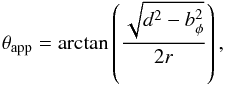 (10)where
“d is the full width half maximum (FWHM) of the Gaussian transverse
profile, r is the distance to the core along the jet axis,
bφ is the beam size along the position
angle φ of the jet-cut, and the quantity
(10)where
“d is the full width half maximum (FWHM) of the Gaussian transverse
profile, r is the distance to the core along the jet axis,
bφ is the beam size along the position
angle φ of the jet-cut, and the quantity
 is the deconvolved FWHM transverse size of the jet” (for more details, see Pushkarev et al. 2012). Note that in this work we use
half opening angles, while Pushkarev et al. (2012)
used full opening angles, which merely differ by a factor of 2.
is the deconvolved FWHM transverse size of the jet” (for more details, see Pushkarev et al. 2012). Note that in this work we use
half opening angles, while Pushkarev et al. (2012)
used full opening angles, which merely differ by a factor of 2.
3.2. Best fits and goodness of fit
We now compare the opening angle data to Eq. (3), where P(Γ) ∝ Γ-1.5 with Γmin = 2 and Γmax = 50. We note, however, that Eq. (3) is insensitive to the form of P(Γ) as we demonstrated in Eq. (7).
We find the best fits using maximum likelihood estimation (MLE) by minimizing the
negative log-likelihood function  (11)where
our data set is
X = (θapp,1,...,θapp,N),
P(Xi,m)
represents P(θapp) evaluated at
θapp = Xi, and
m is a vector representing the free parameters of the distribution
P(θapp). As discussed below, we fit our
data set of N = 133 for six different cases in which the distribution’s
free parameters ranges from three,
m = (ρ,fsh,a),
to only one, m = ρ. When fsh
is not a free parameter it is fixed at 1, and when a is not free it is
fixed at either 2 or 3, as specified below. In all of these cases, we obtain the best fit
parameters
(11)where
our data set is
X = (θapp,1,...,θapp,N),
P(Xi,m)
represents P(θapp) evaluated at
θapp = Xi, and
m is a vector representing the free parameters of the distribution
P(θapp). As discussed below, we fit our
data set of N = 133 for six different cases in which the distribution’s
free parameters ranges from three,
m = (ρ,fsh,a),
to only one, m = ρ. When fsh
is not a free parameter it is fixed at 1, and when a is not free it is
fixed at either 2 or 3, as specified below. In all of these cases, we obtain the best fit
parameters  by numerically minimizing h (Eq. (11)).
To correctly model the fitting error and assess the goodness of fit, we used the
Kolmogorov-Smirnov (KS) statistic LN in
conjunction with the nonparametric bootstrap as described in Feigelson & Babu (2012). Recall that the KS statistic gives a
measure of the distance between the data and the model by finding the maximum distance
between the empirical cumulative distribution function
FN(θapp) and
theoretical cumulative distribution function  ,
i.e.,
,
i.e.,  (12)Here,
for each bootstrap realization, we generate the simulated data X∗
via sampling with replacement, find the best fit parameters
(12)Here,
for each bootstrap realization, we generate the simulated data X∗
via sampling with replacement, find the best fit parameters
 for the simulated data X∗ using the MLE procedure described above,
and then calculate the KS statistic
for the simulated data X∗ using the MLE procedure described above,
and then calculate the KS statistic  from
X∗ and
by using Eq. (12) with an additional bias
correction factor taken into account (see Eq. (3.48) of Feigelson & Babu 2012).
from
X∗ and
by using Eq. (12) with an additional bias
correction factor taken into account (see Eq. (3.48) of Feigelson & Babu 2012).
After iterating the bootstrap B = 2000 times, we obtain confidence
intervals around
by analyzing the distribution of simulated best-fit parameters
and directly compute the 68% and 95% confidence intervals and error contours. The
resulting distribution of the statistic can be used
for model selection by finding the probability p that a value of
LN or greater is observed, assuming that
X is drawn from  .
This is done by defining k as the number of
values that
fulfill the criterion
.
This is done by defining k as the number of
values that
fulfill the criterion  , and then
computing the p-value as
p = k/B. Thus, for
a significance level of α = 0.05, models with p-values
of 0.05 and above are favored by the data (i.e. they cannot be rejected). As discussed
below, we consider six different cases, thus we perform different bootstrap simulations
for each case.
, and then
computing the p-value as
p = k/B. Thus, for
a significance level of α = 0.05, models with p-values
of 0.05 and above are favored by the data (i.e. they cannot be rejected). As discussed
below, we consider six different cases, thus we perform different bootstrap simulations
for each case.
We now apply the above analysis to the data for two different types of models:
No shear model: three cases are considered for our model with no shear, i.e., fsh = 1, depending how the parameter a is treated: (i) a is set to 2; (ii) a = 3; and (iii) a is a free parameter found in the best fit. As it turns out, in case (iii) the best-fit value of a, 6.3, is much higher than the expected fiducial value of 2, and the distribution of best-fit values of a in bootstrap simulations routinely ranges much higher (several tens). In addition, the best values of ρ in the bootstrap simulations is tightly correlated with a, and also ranges widely, suggesting that a and ρ are highly degenerate.
Velocity shear model: here we perform the same analysis and consider the same three cases as above, but with fsh as a free parameter. Thus, ρ and fsh are free parameters and we consider three different cases regarding a: (i) a = 2; (ii) a = 3; and (iii) a as a free parameter to be found in the best fit.
Table 1 gives a summary of our best-fit results, and
Fig. 3 shows a comparison between the data and two
different best-fit models, each with the same number of free parameters (two). The models
that include relativistic velocity shear are clearly favored by the data, as they all have
p-values above 0.05. When shear is included and all the parameters are
varied (the shear (iii) model), the best fit produces a reasonable value of
 (and ρ = 0.21 ± 0.03 and
fsh = 0.33 ± 0.1), which is close to the expected value
of a = 2 from Doppler beaming models and integral source counts of
radio-selected AGN. Encouragingly, the best-fit values for all of the models is
ρ = 0.1−0.2, which is consistent with the values of 0.17 and 0.13
reported in Jorstad et al. (2005) and Pushkarev et al. (2009), respectively. Figure 4 shows the two dimensional error contours for the
shear (iii) model. Since our shear models produce better fits with high
p-values and a reasonable value of a, we conclude that
it is likely that relativistic shear and Doppler beaming play a role in jet appearance. As
our final result for a measurement of Γθj, we report
0.21 ± 0.03 from the shear (iii) model. However, for a more direct comparison between our
value of ρ and that of other researchers, we calculate the expected value
of ρeff(θapp)
(and ρ = 0.21 ± 0.03 and
fsh = 0.33 ± 0.1), which is close to the expected value
of a = 2 from Doppler beaming models and integral source counts of
radio-selected AGN. Encouragingly, the best-fit values for all of the models is
ρ = 0.1−0.2, which is consistent with the values of 0.17 and 0.13
reported in Jorstad et al. (2005) and Pushkarev et al. (2009), respectively. Figure 4 shows the two dimensional error contours for the
shear (iii) model. Since our shear models produce better fits with high
p-values and a reasonable value of a, we conclude that
it is likely that relativistic shear and Doppler beaming play a role in jet appearance. As
our final result for a measurement of Γθj, we report
0.21 ± 0.03 from the shear (iii) model. However, for a more direct comparison between our
value of ρ and that of other researchers, we calculate the expected value
of ρeff(θapp)  (13)where
the parameters of P(θapp) are those for the
shear (iii) model listed in Table 1, and the confidence
interval comes from the bootstrap simulations used to derive the confidence intervals for
the shear (iii) model. Indeed, this value of
⟨ ρeff ⟩ ≈ 0.13 ± 0.02 is consistent with both Pushkarev et al. (2009) and Jorstad et al. (2005).
(13)where
the parameters of P(θapp) are those for the
shear (iii) model listed in Table 1, and the confidence
interval comes from the bootstrap simulations used to derive the confidence intervals for
the shear (iii) model. Indeed, this value of
⟨ ρeff ⟩ ≈ 0.13 ± 0.02 is consistent with both Pushkarev et al. (2009) and Jorstad et al. (2005).
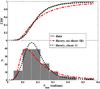 |
Fig. 3 Example best fits for two cases are shown in the form of cumulative distribution functions (CDF, upper panel) and probability density functions (PDF, lower panel). The two cases shown, “no shear (iii)” (dash-dotted line) and “shear (i)” (dotted line), both have the same number of free parameters (two), but the shear (i) model clearly fits the data better. The data is represented as a solid line (upper panel) or histogram (lower panel). |
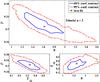 |
Fig. 4 68% and 95% confidence contours from Monte Carlo error analysis for the best-fit parameters ρ, a, and fsh, from the case of shear (iii). The central star shows the MLE of the parameters. We emphasize the a vs. ρ plot since there is a fiducial value for a (=2, vertical dotted line), and ρ has constraints set on it by Jorstad et al. (2005) and Pushkarev et al. (2009). |
Parameter values (both best fit and assigned) for six different cases along with 68% confidence intervals where relevant.
A more rigorous comparison between our best-fit value for ρ and those of other researchers requires a proper error analysis for all of the different measured/inferred values for ρ, both in this paper and in other works. However, in the case of Jorstad et al. (2005) and Pushkarev et al. (2009), the error in their estimated values for θj and Γ for each jet is unknown, as these estimates rely upon highly uncertain model assumptions regarding, for example, equipartition brightness temperature arguments and the equation of component variability with light-crossing times. In addition to this error, it is also possible that AGN jets possess a range of values of ρ, as opposed to our assumption that all jets have the same ρ. These same issues apply to our simple model. More specifically, our confidence limits (see Fig. 4) are probably underestimated since there is considerable uncertainty in our model of velocity shear, our assumption of jet conical geometry, and our assumption that all MOJAVE jets posses the same value of ρ.
4. Discussion
4.1. Relativistic jet physics and Γθj
A variety of physical processes in jets are sensitive to Γθj.
Causal connection implies that θjℳ ≤ 1, where
ℳ = βΓ/(Γsβs)
is the relativistic Mach number, which is the ratio of the jet proper speed to proper
signal speed. (In the Appendix we explain the relationship between
θjℳ, Γθj, and causality). For
jets with a dynamically important magnetic field, the signal speed is the fast
magnetosonic speed, while for jets with no significant magnetic field the signal speed is
the sound speed, which is  for a relativistically hot jet. The fast magnetosonic proper speed is
Γmsβms = σ1/2,
where σ is the magnetization parameter, which is the ratio of Poynting
flux to kinetic flux (Kennel & Coroniti
1984). Beyond the acceleration zone the jet is likely to be in equipartition such
that σ is of the order of unity (e.g., Komissarov et al. 2007). Thus, fiducial jet signal speeds imply that the causal
connection condition for jets is
for a relativistically hot jet. The fast magnetosonic proper speed is
Γmsβms = σ1/2,
where σ is the magnetization parameter, which is the ratio of Poynting
flux to kinetic flux (Kennel & Coroniti
1984). Beyond the acceleration zone the jet is likely to be in equipartition such
that σ is of the order of unity (e.g., Komissarov et al. 2007). Thus, fiducial jet signal speeds imply that the causal
connection condition for jets is 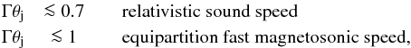 indicating
that AGN jets with the value we have determined here,
Γθj ~ 0.2, are probably causally connected. This verifies the
standard picture of jet production (see Sect. 4.2
and Komissarov et al. 2009), and also implies that
AGN jets are susceptible to various instabilities and reconnection, and are also sensitive
to conditions at the boundary between the jet and the interstellar medium.
indicating
that AGN jets with the value we have determined here,
Γθj ~ 0.2, are probably causally connected. This verifies the
standard picture of jet production (see Sect. 4.2
and Komissarov et al. 2009), and also implies that
AGN jets are susceptible to various instabilities and reconnection, and are also sensitive
to conditions at the boundary between the jet and the interstellar medium.
The particular value of Γθj is also important for instability
development (Narayan et al. 2009), because it gives
a measure of the extent to which jet sidewise expansion inhibits instability growth. Most
global instabilities grow on some comoving signal crossing timescale,
tdyn = Γθjz/(βsc),
where βs is the signal speed and z is the jet
height above the launching region. For Kelvin-Helmholtz instabilities
βs is the sound speed (Perucho et al. 2004; Hardee et al. 2005),
while for current driven kink instabilities βs is the Alfvén
speed (Giannios & Spruit 2006). This
so-called dynamical timescale for the growth of instabilities must be compared to the jet
expansion time
texp = z/(βc),
where if
texp > tdyn
then jet expansion will quench instability growth (Begelman
1998; Giannios & Spruit 2006;
Moll et al. 2008; Spruit 2010). This criterion for instability growth then becomes
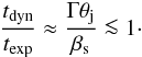 (14)Since
Γθj ~ 0.2, then AGN jet instabilities can grow despite jet
expansion, unless βs ≲ 0.2, which would be below the
relativistic adiabatic sound speed of ~0.6.
(14)Since
Γθj ~ 0.2, then AGN jet instabilities can grow despite jet
expansion, unless βs ≲ 0.2, which would be below the
relativistic adiabatic sound speed of ~0.6.
4.2. Jet acceleration for GRBs vs. AGNs
Long duration GRBs have typical values of Γθj of the order of
10−30 (Panaitescu & Kumar 2002), which is
two orders of magnitude higher than the value we find for AGN jets:
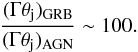 Thus,
it is possible that different physics are at work in GRB jets. Tchekhovskoy et al. (2010) found that a jet acceleration mechanism
(first discovered by Aloy & Rezzolla 2006
and Mizuno et al. 2008) can operate in GRBs in
which a brief period of bulk acceleration occurs upon jet break out into the circumstellar
medium and allows the jet to take on values of Γθj ≫ 1. Komissarov et al. (2010) call this process
rarefaction acceleration, and contrast it to the standard jet
acceleration model of collimation acceleration described in Li et al. (1992) and many other works. Collimation
acceleration entails jet acceleration over an extended distance along the jet (Vlahakis & Konigl 2004) and implies that
Γθj ≤ 1 (Komissarov et al.
2009; Tchekhovskoy et al. 2009). In
contrast, rarefaction acceleration occurs in GRBs because they are initially confined by
the shocked boundary layer in the star until the jet breaks out into the circumstellar
medium, becomes unconfined, and launches a rarefaction wave toward the center of the jet.
If the jet is still magnetically dominated at that point, then this process further
accelerates the jet, and can produce Γθj ≫ 1. Thus, the
dichotomy between GRB jets and AGN jets is nicely explained by the different physical
processes at work in GRB jets (rarefaction acceleration due to jet break out) and AGN jets
(collimation acceleration). Furthermore, as Komissarov et
al. (2010) explain, rarefaction acceleration increases the
Γθj parameter primarily by increasing Γ alone (The increase
in θj is less than 1/Γ). Thus, to the
degree that the typical AGN jet value of Γθj is equal to the
pre-breakout GRB jet value of Γθj, one can infer that
(Γθj)GRB is so much larger than
(Γθj)AGN because of the increase of the GRB jet’s
Γ during the rarefaction acceleration process. Interestingly, this suggests that GRBs have
Γ ≳ 100, which is consistent with the lower limit obtained by requiring that GRB prompt
emission regions be optically thin to gamma-rays with respect to photon-photon pair
production (e.g., Piran 2004).
Thus,
it is possible that different physics are at work in GRB jets. Tchekhovskoy et al. (2010) found that a jet acceleration mechanism
(first discovered by Aloy & Rezzolla 2006
and Mizuno et al. 2008) can operate in GRBs in
which a brief period of bulk acceleration occurs upon jet break out into the circumstellar
medium and allows the jet to take on values of Γθj ≫ 1. Komissarov et al. (2010) call this process
rarefaction acceleration, and contrast it to the standard jet
acceleration model of collimation acceleration described in Li et al. (1992) and many other works. Collimation
acceleration entails jet acceleration over an extended distance along the jet (Vlahakis & Konigl 2004) and implies that
Γθj ≤ 1 (Komissarov et al.
2009; Tchekhovskoy et al. 2009). In
contrast, rarefaction acceleration occurs in GRBs because they are initially confined by
the shocked boundary layer in the star until the jet breaks out into the circumstellar
medium, becomes unconfined, and launches a rarefaction wave toward the center of the jet.
If the jet is still magnetically dominated at that point, then this process further
accelerates the jet, and can produce Γθj ≫ 1. Thus, the
dichotomy between GRB jets and AGN jets is nicely explained by the different physical
processes at work in GRB jets (rarefaction acceleration due to jet break out) and AGN jets
(collimation acceleration). Furthermore, as Komissarov et
al. (2010) explain, rarefaction acceleration increases the
Γθj parameter primarily by increasing Γ alone (The increase
in θj is less than 1/Γ). Thus, to the
degree that the typical AGN jet value of Γθj is equal to the
pre-breakout GRB jet value of Γθj, one can infer that
(Γθj)GRB is so much larger than
(Γθj)AGN because of the increase of the GRB jet’s
Γ during the rarefaction acceleration process. Interestingly, this suggests that GRBs have
Γ ≳ 100, which is consistent with the lower limit obtained by requiring that GRB prompt
emission regions be optically thin to gamma-rays with respect to photon-photon pair
production (e.g., Piran 2004).
4.3. Doppler beaming and θapp
If Γθj is approximately constant in the AGN jet population,
then θapp is an important observable quantity related to
Doppler beaming for two reasons. First, it can serve as a dividing line between highly
beamed (θob < 1/Γ)
jets and not highly beamed jets
(θob > 1/Γ), a
property we exploit in our model of velocity shear in Sect. 2.2. This division conveniently maps onto θapp as
follows: 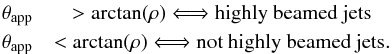 This
implies that jets with
θapp ~ Γθj ~ 0.2 are observed at
the critical angle, thus maximizing the apparent speed of their superluminal components.
This division provides a concise way of explaining the Pushkarev et al. (2009) argument that large-opening angle jets are more highly
Doppler beamed: large opening angle jets with θapp ≳ 0.2 are
all observed within the critical angle and therefore more highly beamed than smaller
θapp jets. Pushkarev et al.
(2009) also find that AGN jets with larger θapp have
a higher Fermi-LAT detection rate, and all jets with
θapp > 0.35 are detected by
Fermi-LAT, implying that Fermi-LAT detected jets tend
to have higher Doppler factors. Notably, this finding is also supported by Kovalev et al. (2009), Savolainen et al. (2010), and Lister et al.
(2009c), who found evidence that radio jets of Fermi-detected AGN are more likely
to have high Doppler factors than are non Fermi-LAT detected sources.
This
implies that jets with
θapp ~ Γθj ~ 0.2 are observed at
the critical angle, thus maximizing the apparent speed of their superluminal components.
This division provides a concise way of explaining the Pushkarev et al. (2009) argument that large-opening angle jets are more highly
Doppler beamed: large opening angle jets with θapp ≳ 0.2 are
all observed within the critical angle and therefore more highly beamed than smaller
θapp jets. Pushkarev et al.
(2009) also find that AGN jets with larger θapp have
a higher Fermi-LAT detection rate, and all jets with
θapp > 0.35 are detected by
Fermi-LAT, implying that Fermi-LAT detected jets tend
to have higher Doppler factors. Notably, this finding is also supported by Kovalev et al. (2009), Savolainen et al. (2010), and Lister et al.
(2009c), who found evidence that radio jets of Fermi-detected AGN are more likely
to have high Doppler factors than are non Fermi-LAT detected sources.
Second, by measuring both a jet’s θapp and its typical
apparent speed
βapp = βsinθob(1 − βcosθob)-1,
we can derive that jet’s Doppler factor, Lorentz factor, and therefore also the viewing
angle, 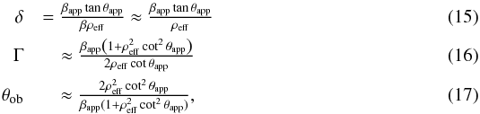 where
where
 is the Doppler factor and β is the jet velocity in units of the speed of
light. Except for Eq. (15), which shows
both the exact and approximate form of δ, the above equations are
approximations that assume Γ ≫ 1 and θob ≪ 1.
is the Doppler factor and β is the jet velocity in units of the speed of
light. Except for Eq. (15), which shows
both the exact and approximate form of δ, the above equations are
approximations that assume Γ ≫ 1 and θob ≪ 1.
Thus, Eqs. ((15)–(17)) demonstrate that, if the spread of ρ (=Γθj) is small enough in the jet population, the measurable quantities βapp and θapp can be useful for calculating intrinsic jet quantities such as the intrinsic brightness temperature and Lorentz factor of jet components. In a future work we intend to explore this new method of deriving a jet’s beaming parameters.
5. Conclusion
We have derived a statistical model of relativistic jet apparent opening angles and fit it to the observed distribution of jet apparent opening angles in the MOJAVE sample. The product of Lorentz factor and intrinsic jet opening angle Γθj is a free parameter in our model and was determined by the best fit to be Γθj ≈ 0.2. We summarize our conclusions as follows.
-
1.
Γθj ~ 0.2 implies that jets are causally connected (see the Appendix), which is predicted by magnetic jet production models. Causal connection also implies that AGN jets are subject to Kelvin-Helmholtz and current-driven (kink) modes, unless the relevant signal speed is ≲Γθjc ~ 0.2c.
-
2.
The value of Γθj for GRB jets is 100 times larger than Γθj for AGN jets. This difference is neatly explained by an acceleration process probably unique to GRBs, wherein a rarefaction wave is launched into the jet after the jet breaks out of its stellar envelope and into the lower pressure circumstellar medium. This is consistent with the high Lorentz factors inferred for GRB jets of Γ ≳ 100.
-
3.
In order to adequately fit the θapp data, we included the effects of relativistic velocity shear and Doppler beaming. Velocity shear affects jets by making blazars appear narrower as their ultra-relativistic inner spine is all that is visible, while jets viewed outside the critical angle 1/Γ appear to have larger jet opening angles. Distinguishing jets based on their critical angle conveniently creates a division between highly beamed jets and not so highly beamed jets that corresponds to whether an individual jet’s apparent opening angles is θapp ≲ Γθj (not highly beamed) or θapp ≳ Γθj (highly beamed).
-
4.
Assuming Γθj is mostly constant across the AGN jet population, then a jet’s Doppler factor, Lorentz factor, and viewing angle can be calculated if the observable values of apparent jet opening angle θapp and the apparent speed of the jet components βapp are known. This is shown in Eqs. ((15)–(17)).
Another type of causal connection that we do not discuss in this paper is the ability of a disturbance to communicate upstream with the jet’s central engine. For super-fast magnetosonic jets, these disturbances cannot propagate back to the central engine.
Acknowledgments
ECB thanks M. Böck, M. Zamaninasab, M. Lister, M. Lyutikov, and D. Giannios for valuable discussions. A.B.P. was supported by the “Non-stationary processes in the Universe” Program of the Presidium of the Russian Academy of Sciences. Y.Y.K. was supported by the Russian Foundation for Basic Research (project 12-02-33101), the Dynasty Foundation, and the Research Program OFN-17 of the Division of Physics, Russian Academy of Sciences. This research has made use of data from the MOJAVE database that is maintained by the MOJAVE team (Lister et al. 2009a).
References
- Aloy, M. A., & Rezzolla, L. 2006, ApJ, 640, L115 [NASA ADS] [CrossRef] [Google Scholar]
- Aloy, M. A., Gómez, J. L., Ibáñez, J. M., et al. 2000, ApJ, 528, L85 [Google Scholar]
- Attridge, J. M., Roberts, D. H., & Wardle, J. F. C. 1999, ApJ, 518, L87 [NASA ADS] [CrossRef] [Google Scholar]
- Begelman, M. C. 1998, ApJ, 493, 291 [NASA ADS] [CrossRef] [Google Scholar]
- Beskin, V. S. 2010, Phys. Uspekhi, 53, 1197 [Google Scholar]
- Chiaberge, M., Celotti, A., Capetti, A., & Ghisellini, G. 2000, A&A, 358, 104 [NASA ADS] [Google Scholar]
- Clausen-Brown, E., Lyutikov, M., & Kharb, P. 2011, MNRAS, 415, 2081 [NASA ADS] [CrossRef] [Google Scholar]
- Cohen, M. H. 1989, in BL Lac Objects, eds. L. Maraschi, T. Maccacaro, & M.-H. Ulrich (Berlin: Springer), 13 [Google Scholar]
- Feigelson, E. D., & Babu, G. J. 2012, Modern Statistical Methods for Astronomy (Cambridge University Press) [Google Scholar]
- Giannios, D. 2013, MNRAS, 431, 355 [NASA ADS] [CrossRef] [Google Scholar]
- Giannios, D., & Spruit, H. C. 2006, A&A, 898, 887 [NASA ADS] [CrossRef] [EDP Sciences] [Google Scholar]
- Hardee, P. E., Walker, R. C., & Gómez, J. L. 2005, ApJ, 620, 646 [NASA ADS] [CrossRef] [Google Scholar]
- Homan, D. C., Kadler, M., Kellermann, K. I., et al. 2009, ApJ, 706, 1253 [NASA ADS] [CrossRef] [Google Scholar]
- Hovatta, T., Valtaoja, E., Tornikoski, M., & Lähteenmäki, A. 2009, A&A, 537, 527 [CrossRef] [EDP Sciences] [Google Scholar]
- Jorstad, S. G., Marscher, A. P., Lister, M. L., et al. 2005, AJ, 130, 1418 [NASA ADS] [CrossRef] [Google Scholar]
- Kennel, C. F., & Coroniti, F. V. 1984, ApJ, 283, 694 [NASA ADS] [CrossRef] [Google Scholar]
- Kinoshita, S., Sendouda, Y., & Takahashi, K. 2004, Phys. Rev. D, 70, 123006 [NASA ADS] [CrossRef] [Google Scholar]
- Kohler, S., Begelman, M. C., & Beckwith, K. 2012, MNRAS, 422, 2282 [NASA ADS] [CrossRef] [Google Scholar]
- Komissarov, S. S., Barkov, M. V., Vlahakis, N., & Königl, A. 2007, MNRAS, 380, 51 [NASA ADS] [CrossRef] [Google Scholar]
- Komissarov, S. S., Vlahakis, N., Königl, A., & Barkov, M. V. 2009, MNRAS, 394, 1182 [NASA ADS] [CrossRef] [Google Scholar]
- Komissarov, S. S., Vlahakis, N., & Königl, A. 2010, MNRAS, 407, 17 [NASA ADS] [CrossRef] [Google Scholar]
- Konigl, A. 1980, Phys. Fluids, 23, 1083 [NASA ADS] [CrossRef] [Google Scholar]
- Kovalev, Y. Y., Kellermann, K. I., Lister, M. L., et al. 2005, AJ, 130, 2473 [NASA ADS] [CrossRef] [Google Scholar]
- Kovalev, Y. Y., Lister, M. L., Homan, D. C., & Kellermann, K. I. 2007, ApJ, 668, L27 [NASA ADS] [CrossRef] [Google Scholar]
- Kovalev, Y. Y., Aller, H. D., Aller, M. F., et al. 2009, ApJ, 696, L17 [NASA ADS] [CrossRef] [Google Scholar]
- Laing, R. A., & Bridle, A. H. 2004, MNRAS, 348, 1459 [NASA ADS] [CrossRef] [Google Scholar]
- Li, Z., Chiueh, T., & Begelman, M. C. 1992, ApJ, 394, 459 [NASA ADS] [CrossRef] [Google Scholar]
- Lind, K., & Blandford, R. 1985, ApJ, 295, 358 [NASA ADS] [CrossRef] [Google Scholar]
- Lister, M. L., & Homan, D. C. 2005, AJ, 130, 1389 [NASA ADS] [CrossRef] [Google Scholar]
- Lister, M. L., Aller, H. D., Aller, M. F., et al. 2009a, AJ, 137, 3718 [NASA ADS] [CrossRef] [Google Scholar]
- Lister, M. L., Cohen, M. H., Homan, D. C., et al. 2009b, AJ, 138, 1874 [NASA ADS] [CrossRef] [Google Scholar]
- Lister, M. L., Homan, D. C., Kadler, M., et al. 2009c, ApJ, 696, L22 [NASA ADS] [CrossRef] [Google Scholar]
- Lister, M. L., Aller, M. F., Aller, H. D., et al. 2013, AJ, 146, 120 [NASA ADS] [CrossRef] [Google Scholar]
- Lyutikov, M., Pariev, V. I., & Blandford, R. D. 2003, ApJ, 597, 998 [NASA ADS] [CrossRef] [Google Scholar]
- McKinney, J. C. 2006, MNRAS, 368, 1561 [NASA ADS] [CrossRef] [Google Scholar]
- Miller-Jones, J. C. A., Fender, R. P., & Nakar, E. 2006, MNRAS, 367, 1432 [NASA ADS] [CrossRef] [Google Scholar]
- Mizuno, Y., Hardee, P., Hartmann, D. H., et al. 2008, ApJ, 672, 72 [NASA ADS] [CrossRef] [Google Scholar]
- Moll, R., Spruit, H. C., & Obergaulinger, M. 2008, A&A, 630, 621 [NASA ADS] [CrossRef] [EDP Sciences] [Google Scholar]
- Nakar, E., Piran, T., & Waxman, E. 2003, JCAP, 10 [Google Scholar]
- Nalewajko, K., & Sikora, M. 2009, MNRAS, 392, 1205 [NASA ADS] [CrossRef] [Google Scholar]
- Narayan, R., Li, J., & Tchekhovskoy, A. 2009, ApJ, 697, 1681 [NASA ADS] [CrossRef] [Google Scholar]
- Owen, F. N., Hardee, P. E., & Cornwell, T. J. 1989, ApJ, 340, 698 [NASA ADS] [CrossRef] [Google Scholar]
- Panaitescu, A., & Kumar, P. 2002, ApJ, 571, 779 [NASA ADS] [CrossRef] [Google Scholar]
- Perlman, E. S., Biretta, J. A., Zhou, F., et al. 1999, ApJ, 117, 2185 [Google Scholar]
- Perucho, M., Hanasz, M., Martí, J. M., & Sol, H. 2004, A&A, 427, 415 [NASA ADS] [CrossRef] [EDP Sciences] [Google Scholar]
- Perucho, M., Kovalev, Y. Y., Lobanov, A. P., et al. 2012, ApJ, 749, 55 [NASA ADS] [CrossRef] [EDP Sciences] [Google Scholar]
- Piran, T. 2004, Rev. Mod. Phys., 76, 1143 [Google Scholar]
- Pushkarev, A. B., & Kovalev, Y. Y. 2012, A&A, 544, A34 [NASA ADS] [CrossRef] [EDP Sciences] [Google Scholar]
- Pushkarev, A. B., Kovalev, Y. Y., Lister, M. L., & Savolainen, T. 2009, A&A, 507, L33 [NASA ADS] [CrossRef] [EDP Sciences] [Google Scholar]
- Pushkarev, A. B., Lister, M. L., Kovalev, Y. Y., & Savolainen, T. 2012, Proceedings of Fermi & Jansky – Our Evolving Understanding of AGN – eConf C1111101 [arXiv:1205.0659] [Google Scholar]
- Savolainen, T., Homan, D. C., Hovatta, T., et al. 2010, A&A, 512, A24 [NASA ADS] [CrossRef] [EDP Sciences] [Google Scholar]
- Spruit, H. C. 2010, Theory of Magnetically Powered Jets, Lect. Notes Phys., 794, 233 [Google Scholar]
- Swain, M. R., & Bridle, A. H. 1998, ApJ, 507, L29 [NASA ADS] [CrossRef] [Google Scholar]
- Tavecchio, F., & Ghisellini, G. 2008, MNRAS, 385, L98 [NASA ADS] [CrossRef] [Google Scholar]
- Tchekhovskoy, A., McKinney, J. C., & Narayan, R. 2009, ApJ, 699, 1789 [NASA ADS] [CrossRef] [Google Scholar]
- Tchekhovskoy, A., Narayan, R., & McKinney, J. C. 2010, New Astron., 15, 749 [Google Scholar]
- Urry, C. M., & Padovani, P. 1991, ApJ, 371, 60 [NASA ADS] [CrossRef] [Google Scholar]
- Urry, C. M., & Shafer, R. A. 1984, ApJ, 280, 569 [NASA ADS] [CrossRef] [Google Scholar]
- Vermeulen, R. C., & Cohen, M. H. 1994, ApJ, 430, 467 [NASA ADS] [CrossRef] [Google Scholar]
- Vlahakis, N., & Konigl, A. 2004, ApJ, 605, 656 [NASA ADS] [CrossRef] [Google Scholar]
- Zakamska, N. L., Begelman, M. C., & Blandford, R. D. 2008, ApJ, 679, 990 [NASA ADS] [CrossRef] [Google Scholar]
Appendix A: Causal connection and Γθj
Here we discuss two different criteria for defining whether or a not a jet is causally connected for the simplistic case of a jet with radial velocity streamlines of constant speed. For jets with velocity shear, as we posit in this work, causal connection is more complicated than we have presented below, although we expect the following discussion to be approximately correct. First, the relativistic Mach number ℳ = βΓ/(βsΓs) (Konigl 1980) is sometimes used to define causal connection for supersonic jets by requiring θjℳ < 1, or Γθj < Γsβs/β (e.g., Komissarov et al. 2009). Second, causally connected jets are sometimes defined as those for which Γθj < 1 (e.g., Zakamska et al. 2008). We note that for relativistic jets with β ≈ 1 and an ultra-relativistic equation of state where the proper sound speed is Γsβs = 2− 1/2 ≈ 0.71, both of these causality criteria resemble one another: Γθj < 0.71 for the relativistic Mach number approach, and Γθj < 1 for the other. However, for magnetically dominated plasmas, the fast magnetosonic speed can approach the speed of light, thus no upper bound can be placed on Γsβs and these two criteria for causal connection give contradictory answers. Thus, a jet can have any value of Γθj and still in principle be causally connected, provided it is magnetically dominated enough. In particular, for jets with magnetization σ (Kennel & Coroniti 1984), the proper Alfvén speed is ΓAβA = σ1/2, thus the Mach number condition for the jet to be causally connected is Γθj < σ1/2 (e.g., Komissarov et al. 2009). Jets can then be causally connected even though Γθj ≫ 1, as long as σ is large enough (high σ implies the jet is Poynting flux dominated). Below, we discuss why these two criteria are different and conclude that the relativistic Mach angle analysis is usually the more appropriate criterion, even though it is only approximate.
θjℳ < 1 criterion: This criterion is only relevant for highly supersonic or supermagnetosonic jets, since for subsonic or transonic jets there is no limit on wave propagation.
The relativistic Mach number can be derived by assuming a flow with parallel velocity streamlines and by analyzing the observer frame angle a sound wave can make with respect to the flow direction, tanχ = β⊥/β∥. The relativistic Mach angle is then found by maximizing χ by varying χ′, the rest frame angle between the flow direction and the sound wave direction. This procedure gives cosχ′ = −βs/β and a maximum angle of sinχmax = 1/ℳ (Konigl 1980). Thus, χmax represents the largest observer frame angle a sound wave can make with respect to a supersonic flow. For this reason, jets where θj > χmax are assumed to be out of causal contact with themselves. However, this Mach angle analysis assumes a flow of parallel velocity streamlines, something that is not the case for conical jets.
For conical jets, jet sidewise expansion lengthens the signal crossing time compared to a
flow with parallel streamlines (e.g., a cylindrical jet). Causal connection can be
analyzed by making a simple estimate of a conical jet’s signal crossing time, assuming the
signal propagates at a speed βs in the local fluid rest frame
and makes an angle χ′ between the jet comoving frame signal
wave propagation direction and the local fluid streamline. We also assume that the jet
flow is radial with a half-opening angle of θj and a constant
Lorentz factor of Γ. In the observer frame the wave has a speed parallel to the local
streamline of  (A.1)and
a perpendicular speed of
(A.1)and
a perpendicular speed of  (A.2)For
simplicity we assume the emitted wave trajectory is such that
χ′ is constant. If the radial coordinate (centered on the
jet’s central engine) of the wave is r, then
dr = βrcdt.
In a time dt, the wave propagates in the polar direction an arc length of
ds = βθcdt.
In terms of polar angle, then, the signal propagation can be written as
dθ = βθcdt/r,
which, combined with the
dr = βrcdt,
can be solved for the time it takes for a signal to propagate through a polar angle
θj,
(A.2)For
simplicity we assume the emitted wave trajectory is such that
χ′ is constant. If the radial coordinate (centered on the
jet’s central engine) of the wave is r, then
dr = βrcdt.
In a time dt, the wave propagates in the polar direction an arc length of
ds = βθcdt.
In terms of polar angle, then, the signal propagation can be written as
dθ = βθcdt/r,
which, combined with the
dr = βrcdt,
can be solved for the time it takes for a signal to propagate through a polar angle
θj,  (A.3)where
r0 is the radial location of the initial wave emission. We
note that a different form of Eq. (A.3)
was derived in Kinoshita et al. (2004) and a
similar result was also found in Nakar et al.
(2003). If in the observer frame a sound wave has a trajectory such that
χ = 1/ℳ (i.e.,
χ′ = −βs/β),
then
βr/βθ ≈ ℳ
and βr ≈ β, yielding the
differential equation
dθ = (ℳr)-1dr. This
differential equation has the solution for polar angle through which the signal propagates
of
θ(r) = ℳ-1ln(r/r0)
with the associated signal crossing time of
(A.3)where
r0 is the radial location of the initial wave emission. We
note that a different form of Eq. (A.3)
was derived in Kinoshita et al. (2004) and a
similar result was also found in Nakar et al.
(2003). If in the observer frame a sound wave has a trajectory such that
χ = 1/ℳ (i.e.,
χ′ = −βs/β),
then
βr/βθ ≈ ℳ
and βr ≈ β, yielding the
differential equation
dθ = (ℳr)-1dr. This
differential equation has the solution for polar angle through which the signal propagates
of
θ(r) = ℳ-1ln(r/r0)
with the associated signal crossing time of  (A.4)assuming
ℳ ≫ 1. Equation (A.4) implies that jets
for which θjℳ ≫ 1 have
tcross ≈ (r0/c)exp(θjℳ),
effectively making such jets fall out of causal contact in the sense that the dynamic time
is longer than the jet expansion time
r0/c by a factor
exp(θjℳ).
(A.4)assuming
ℳ ≫ 1. Equation (A.4) implies that jets
for which θjℳ ≫ 1 have
tcross ≈ (r0/c)exp(θjℳ),
effectively making such jets fall out of causal contact in the sense that the dynamic time
is longer than the jet expansion time
r0/c by a factor
exp(θjℳ).
Accelerating conical jets are different in that they can have a causal horizon that
depends on the details of jet acceleration (Kinoshita et
al. 2004). An accelerating supersonic jet will have an increasing proper speed
and a decreasing (or constant) proper signal speed, which we parameterize as
ℳ = ℳ0(r/r0)b.
For a signal emitted at r0 that propagates at the Mach angle
relative to the local fluid streamline, then
dθ = (ℳr)-1dr has the
asymptotic solution  (A.5)That
is, disturbances located at radius r0 will propagate through a
polar angle θ∞ as r → ∞. Thus, in this
circumstance, the causal connection criterion becomes
θjℳ(r) < b-1.
(A.5)That
is, disturbances located at radius r0 will propagate through a
polar angle θ∞ as r → ∞. Thus, in this
circumstance, the causal connection criterion becomes
θjℳ(r) < b-1.
Γθj < 1 criterion: We
assume an initially cylindrical jet with speed β ≈ 1 and associated
Lorentz factor Γ ≫ 1, and let the radius of the cylindrical flow suddenly begin to expand
in the flow rest frame with velocity  perpendicular
to the symmetry axis. Transforming back into the observer frame then gives
perpendicular
to the symmetry axis. Transforming back into the observer frame then gives
 , the
small angle the velocity stream lines make with the jet axis is now
, the
small angle the velocity stream lines make with the jet axis is now
 (A.6)The
requirement that the jet cross section expands at less than the speed of light
(A.6)The
requirement that the jet cross section expands at less than the speed of light
 implies
that (Zakamska et al. 2008)
implies
that (Zakamska et al. 2008)
 (A.7)Thus,
requiring that Γθj < 1 is an important
constraint for jet flows that are initially close to cylindrical, and for some reason
undergo expansion. We note, however, that this constraint is not important for flows that
are initially not collimated, such as the highly relativistic equatorial outflows from
pulsars that power pulsar wind nebulae (Kennel &
Coroniti 1984).
(A.7)Thus,
requiring that Γθj < 1 is an important
constraint for jet flows that are initially close to cylindrical, and for some reason
undergo expansion. We note, however, that this constraint is not important for flows that
are initially not collimated, such as the highly relativistic equatorial outflows from
pulsars that power pulsar wind nebulae (Kennel &
Coroniti 1984).
Alternatively, Γθj can be an important quantity if the sound
wave emission direction in the local rest frame is defined as perpendicular to the local
flow direction, i.e.,
χ′ = π/2, as could be
the case if the wave is restricted to a thin spherical shell (which may be relevant for
GRBs, Lyutikov et al. 2003; Kinoshita et al. 2004), so that
βθ = βs/Γ
and βr = β. In this case,
the sound crossing time from Eq. (A.3)
becomes  (A.8)For
jets with β ≈ 1, βs ≈ 1, and
Γθj ≫ 1, then
tcross ≈ (r0/c)exp(Γθj),
showing that in this case Γθj plays the same role that
θjℳ does in the general case for determining an effective
causal condition.
(A.8)For
jets with β ≈ 1, βs ≈ 1, and
Γθj ≫ 1, then
tcross ≈ (r0/c)exp(Γθj),
showing that in this case Γθj plays the same role that
θjℳ does in the general case for determining an effective
causal condition.
All Tables
Parameter values (both best fit and assigned) for six different cases along with 68% confidence intervals where relevant.
All Figures
|
Fig. 1 Meridional slice of a jet illustrating two cases: (i) jets aligned close to the line of sight where emission is dominated by the fast inner spine; and (ii) more misaligned jets where the emission from outer slower layers contributes as well. |
| In the text | |
|
Fig. 2 Doppler factor and ρeff as a function of a jet’s apparent half-opening angle θapp. The semi-logarithmic Doppler factor plot in the upper panel is for a jet with Γ = 10 and ρ = 0.21, and uses Eq. (4) to convert θapp to θob. The lower panel plot shows ρeff as a function of θapp from Eq. (9) using ρ = 0.21 and fsh = 0.33, the best fit values found in Sect. 3.2. |
| In the text | |
|
Fig. 3 Example best fits for two cases are shown in the form of cumulative distribution functions (CDF, upper panel) and probability density functions (PDF, lower panel). The two cases shown, “no shear (iii)” (dash-dotted line) and “shear (i)” (dotted line), both have the same number of free parameters (two), but the shear (i) model clearly fits the data better. The data is represented as a solid line (upper panel) or histogram (lower panel). |
| In the text | |
|
Fig. 4 68% and 95% confidence contours from Monte Carlo error analysis for the best-fit parameters ρ, a, and fsh, from the case of shear (iii). The central star shows the MLE of the parameters. We emphasize the a vs. ρ plot since there is a fiducial value for a (=2, vertical dotted line), and ρ has constraints set on it by Jorstad et al. (2005) and Pushkarev et al. (2009). |
| In the text | |
Current usage metrics show cumulative count of Article Views (full-text article views including HTML views, PDF and ePub downloads, according to the available data) and Abstracts Views on Vision4Press platform.
Data correspond to usage on the plateform after 2015. The current usage metrics is available 48-96 hours after online publication and is updated daily on week days.
Initial download of the metrics may take a while.