| Issue |
A&A
Volume 688, August 2024
|
|
|---|---|---|
| Article Number | A94 | |
| Number of page(s) | 18 | |
| Section | Astrophysical processes | |
| DOI | https://doi.org/10.1051/0004-6361/202449790 | |
| Published online | 07 August 2024 | |
Jet collimation and acceleration in the flat spectrum radio quasar 1928+738
1
Department of Physics and Astronomy, Seoul National University, Gwanak-gu, Seoul 08826, Republic of Korea
e-mail: This email address is being protected from spambots. You need JavaScript enabled to view it.
2
School of Space Research, Kyung Hee University, 1732 Deogyeong-daero, Giheung-gu, Yongin-si, Gyeonggi-do 17104, Republic of Korea
e-mail: This email address is being protected from spambots. You need JavaScript enabled to view it.
3
National Institute of Technology, Hachinohe College, 16-1 Uwanotai, Tamonoki, Hachinohe, Aomori 039-1192, Japan
4
Institute of Astronomy and Astrophysics, Academia Sinica, PO Box 23-141 Taipei 10617, Taiwan
5
Graduate School of Science, Nagoya City University, Yamanohata 1, Mizuho-cho, Mizuho-ku, Nagoya, 467-8501 Aichi, Japan
e-mail: This email address is being protected from spambots. You need JavaScript enabled to view it.
6
Mizusawa VLBI Observatory, National Astronomical Observatory of Japan, 2-12 Hoshigaoka, Mizusawa, Oshu, Iwate 023-0861, Japan
7
Department of Astronomical Science, The Graduate University for Advanced Studies (SOKENDAI), 2-21-1 Osawa, Mitaka, Tokyo 181-8588, Japan
8
SNU Astronomy Research Center, Seoul National University, Gwanak-gu, Seoul 08826, Republic of Korea
Received:
29
February
2024
Accepted:
2
May
2024
Abstract
Using time-resolved multifrequency Very Long Baseline Array data and new KaVA (KVN and VERA Array) observations, we study the structure and kinematics of the jet of the flat spectrum radio quasar (FSRQ) 1928+738. We find two distinct jet geometries as a function of distance from the central black hole, with the inner jet having a parabolic shape, indicating collimation, and the outer jet having a conical shape, indicating free expansion of the jet plasma. Jet component speeds display a gradual outward acceleration up to a bulk Lorentz factor Γmax ≈ 10 followed by a deceleration further downstream. The location of the acceleration zone matches the region where the jet collimation occurs. Therefore, this is the first direct observation of an acceleration and collimation zone (ACZ) in an FSRQ. The ACZ terminates approximately at a distance of 5.6 × 10⁶ gravitational radii, which is in good agreement with the sphere of gravitational influence of the supermassive black hole, implying that the physical extent of the ACZ is controlled by the black hole gravity. Our results suggest that confinement by an external medium is responsible for the jet collimation and that the jet is accelerated by converting Poynting flux energy to kinetic energy.
Key words: accretion / accretion disks / techniques: high angular resolution / techniques: interferometric / galaxies: active / galaxies: jets / quasars: individual: 1928+738
© The Authors 2024
 Open Access article, published by EDP Sciences, under the terms of the Creative Commons Attribution License (https://creativecommons.org/licenses/by/4.0), which permits unrestricted use, distribution, and reproduction in any medium, provided the original work is properly cited.
This article is published in open access under the Subscribe to Open model. This email address is being protected from spambots. You need JavaScript enabled to view it. to support open access publication.
1. Introduction
A fraction (∼10%) of active galactic nuclei (AGNs) have highly collimated relativistic jets (Urry & Padovani 1995). It is now widely believed that these jets are launched in the vicinity of supermassive black holes (SMBHs) at the center of their host galaxies. An interplay of the magnetic field, accreted gas, and the rotation of the black hole itself (Blandford & Znajek 1977) and/or the accretion disk (Blandford & Payne 1982) produces the momentum and energy required for the formation of jets. The parsec and kiloparsec scale properties of AGN jets have been intensively studied theoretically and observationally for more than five decades (see Blandford et al. 2019; Hada 2019, for a review).
A magnetically driven jet (Blandford & Znajek 1977; Blandford & Payne 1982) is expected to be accelerated to highly relativistic speeds by a magnetohydrodynamic (MHD) conversion of Poynting flux to kinetic energy (e.g., Vlahakis & Königl 2004). This process is efficient if the bulk flow and the poloidal magnetic field lines therein are collimated by the magnetic nozzle effect (e.g., Camenzind 1987; Li et al. 1992; Begelman & Li 1994; Vlahakis 2015), implying that the bulk jet acceleration is intimately associated with jet collimation. It has been suggested that a combined acceleration and collimation zone (ACZ) is formed at distances of ≲105 − 106 gravitational radii (Rg) from the black hole (e.g., Meier et al. 2001; Komissarov et al. 2007; Marscher et al. 2008). Numerous high-resolution observations with Very Long Baseline Interferometry (VLBI) have been performed toward AGN jets to examine the ACZ, which requires resolving the jet structure over a wide range of physical scales.
The existence of an ACZ was confirmed in the nearby radio galaxy M 87, Junor et al. (1999) found that the M 87 jet is being collimated at a distance of ≲10 pc, and Asada & Nakamura (2012) reported that the jet collimation is sustained up to ∼105 Rg, breaking at around the Bondi radius. This suggests that the gas accreted onto the central black hole, which is stratified by the black hole’s gravity, might be responsible for shaping a relativistic AGN jet into a parabolic stream. This interpretation is consistent with the theoretical expectation that a jet requires confinement by an ambient medium to be collimated (e.g., Lyubarsky 2009). Likewise, the acceleration of the jet takes place inside the Bondi radius (Nakamura & Asada 2013; Asada et al. 2014; Mertens et al. 2016; Hada et al. 2017; Walker et al. 2018; Park et al. 2019a) and transits into a slow deceleration beyond the Bondi radius (Biretta et al. 1995, 1999; Meyer et al. 2013).
The general understanding of jet collimation has evolved greatly since the jets of other radio-loud AGNs have been extensively investigated with the same approach. An active collimation at ≲104 Rg (e.g., Giovannini et al. 2018; Boccardi et al. 2019) and a transition into a free expansion phase further downstream (see Tseng et al. 2016; Akiyama et al. 2018; Nakahara et al. 2018, 2020; Hada et al. 2018; Traianou et al. 2020; Kovalev et al. 2020; Park et al. 2021; Boccardi et al. 2021; Burd et al. 2022; Okino et al. 2022) have been discovered in an increasing number of AGN jets.
Nonetheless, jet acceleration within the collimation zone is mostly unexplored, except for a few sources. Hence, several key questions such as how and where the bulk acceleration terminates or what the maximum speed Γmax is remain unclear. This is partly due to a lack of monitoring observations. Indeed, a robust analysis of the jet velocity field requires multi-epoch VLBI observations at a high cadence. To date, jet acceleration and collimation in the same region, and thus a genuine ACZ, have been observed only in two Fanaroff-Riley type I (FR I; Fanaroff & Riley 1974) radio galaxies (M 87; Asada & Nakamura 2012; Asada et al. 2014 and NGC 315; Park et al. 2021; Boccardi et al. 2021; Ricci et al. 2022) and one narrow-line Seyfert 1 (NLS1) galaxy (1H 0323+342; Hada et al. 2018). Notably, while the sample size has increased slowly, so far there has been no detailed study of the interplay of jet acceleration and collimation in a flat spectrum radio quasar (FSRQ), the FR II-like AGN sub-class.
The FSRQ 1928+738 (also known as 4C +73.18) is located at a redshift of 0.302 (Lawrence et al. 1986) and hosts a SMBH with a mass of M• ≈ 3.7 × 10⁸ M⊙ in its center (see Park & Trippe 2017, and the references therein). It is noteworthy that 1928+738 is one of very few “misaligned” FSRQs with an unusually large viewing angle of θv ≃ 10° −15° between the jet and the line of sight (Lähteenmäki & Valtaoja 1999; Hovatta et al. 2009; Liodakis et al. 2018). When adopting θv = 13.2° (see Sect. 3.6), one finds a convenient conversion between angular scale and deprojected physical scale: 1 mas ∼106 Rg. Therefore, 1928+738 is one of the best FSRQ targets to directly investigate its putative jet ACZ with (sub-)mas VLBI observations.
While the Very Large Array (VLA)/MERLIN observations show a two-sided jet and structure on arcsecond (and thus kiloparsec) scales (Johnston et al. 1987; Hummel et al. 1992), the Very Long Baseline Array (VLBA) images show only a one-sided jet extending to the south (Eckart et al. 1985). At parsec scales, it has long been known that the 1928+738 jet shows apparently superluminal motion. Interestingly, previous well-sampled observations (e.g., Homan et al. 2001; Kellermann et al. 2004) found a hint of a gradual increase in jet speed versus distance. Several studies (e.g., Kun et al. 2014; Homan et al. 2015; Lister et al. 2021) have found consistent maximum proper motions (βapp ≈ 8), but they disagree on the location of the fastest jet speed. The suggested location spans ≈1 to ≈13 mas from the origin of the jet.
In this paper, we investigate the jet collimation and acceleration of 1928+738 in detail. We present the results of multifrequency VLBI observations. Based on single-epoch deep imaging and multi-epoch dense monitoring, we explore the structural evolution of the radio jet, its kinematics, and variability. We note that a dedicated spectral analysis will be presented in a forthcoming paper. Our paper is structured as follows: In Sect. 2, we describe archival data, our new observations, and the data reduction. In Sects. 3 and 4, our results and analysis are presented and discussed. Finally, we summarize the results and implications of our study in Sect. 5. Throughout this paper, we adopt a cosmology with the following parameters: H0 = 70 km s−1 Mpc−1, Ωm = 0.3, ΩΛ = 0.7. This results in a luminosity distance of 1565 Mpc, and an angular-to-linear scale conversion of 4.47 pc mas−1 in projection. Thus, a proper motion of 1 mas yr−1 translates to an apparent superluminal speed of 19 c.
2. Data and data reduction
In this section, we describe VLBI data taken from various public archives as well as new observations of FSRQ 1928+738. The archival data are systematically categorized according to their respective purposes.
2.1. VLBA archival data for jet collimation analysis
We searched the National Radio Astronomy Observatory (NRAO) archive for VLBA data suitable for a study of jet collimation. We selected the VLBA project BS266 in which 1928+738 was observed for over 10 h utilizing nine VLBA stations, except Saint Croix (VLBA-SC). The observations were made at five frequencies: 1.6 GHz, 4 GHz, 7 GHz, 15 GHz, and 24 GHz. We provide a summary of the data in Table 1.
VLBA project BS266 in 2018 June.
2.2. VLBA archival data for jet kinematics analysis
We obtained multi-epoch VLBI data from various archival databases (summarized in Table 2). The S- and X-band (2.3 and 7.6−8.6 GHz) data sets are from the Astrogeo VLBI FITS image database1, which contains extensive surveys, such as several versions of the VLBA Calibrator Survey (VCS; Petrov et al. 2006, 2008; Kovalev et al. 2007; Petrov 2021) and the VLBI 2MASS Survey (V2M; Condon et al. 2011). In total, we analyzed the calibrated data observed over eight and 16 epochs from 2005 to 2019 for the S- and X-bands, respectively. We refer the readers to Pushkarev & Kovalev (2012) for detailed descriptions of the data and the data processing.
Summary of data sets used for jet kinematics.
The 15 GHz data set is from the MOJAVE database2 (e.g., Lister et al. 2018). We analyzed 14 epochs of calibrated visibility data from 2016 January to 2019 August. We note that we only considered the total intensity, not the polarized emission.
2.3. KaVA 43 GHz data
In addition to the VLBA archival data mentioned above, we also performed a new dedicated observing program on 1928+738 at 43 GHz. We conducted high cadence (approximately monthly) monitoring with the KVN3 and VERA4 Array (KaVA; Niinuma et al. 2014; Hada et al. 2017; Park et al. 2019a; Cho et al. 2022), which serves as a core array in the East Asian VLBI Network (EAVN; Wajima et al. 2016; An et al. 2018; Cui et al. 2023). In each session, all seven stations were scheduled by default in a 6- to 8-h track. One or two stations were missing occasionally, due to local issues such as bad weather or system failures (see Table 3). On 2018 January 22, because of the loss of the VERA-Mizusawa and KVN-Tamna stations, the data quality was severely compromised, leading to the exclusion of the data. In total, we obtained 22 epochs of data from 2017 February to 2019 January. We summarize our KaVA observations in Table 3.
Summary of KaVA monitoring for 1928+738 at 43 GHz.
All observations used the single polarization (left-hand circular only) mode with 2-bit quantization. The data were recorded at a rate of 1 Gbps in eight sub-bands of 32 MHz width each and correlated at the Korea-Japan Correlation Center using the Daejeon hardware correlator (Lee et al. 2015a).
2.4. Data reduction
After correlation, the raw data were calibrated by using the NRAO Astronomical Image Processing System (AIPS; Greisen 2003). We applied the standard KaVA and VLBA data reduction procedures (Niinuma et al. 2014; Oh et al. 2015; Hada et al. 2017, 2020; Kino et al. 2018; Lee et al. 2019; Park et al. 2019a; Wajima et al. 2020) for the initial phase, bandpass, and amplitude calibrations. A priori, the amplitude calibration was applied by using the gain curve and system temperature of each antenna. Notably, the VLBA data underwent a manual atmospheric opacity correction using the APCAL procedure in AIPS. This step was necessary only for VLBA data, as the KaVA system temperatures were already opacity corrected during the observations. Additionally, to correct the multiple losses stemming from signal processing in the observing system and the characteristics in the Daejeon correlator, the visibility amplitudes of the KaVA data were scaled up by a factor of 1.3 (Lee et al. 2015b). Iterative CLEAN and self-calibration processes were performed in the Difmap software (Shepherd 1997) for imaging.
3. Analysis and results
3.1. Multifrequency jet images on various scales
We analyzed the radial profiles of the width and velocity field of the jet of 1928+738 to investigate its collimation and acceleration. All displacements and directions were measured with respect to the core for analysis. Throughout this paper, we use the conventional label “core” for the innermost and compact feature of the radio jet. The core is presumably stationary and thus used as a reference point. We note that all images are shifted to place the core at the origin (RA, Dec) = (0, 0) of each map. However, we also note that the physical core position may depend on the observing frequency (see Sect. 3.2).
We present VLBA and KaVA images of FSRQ 1928+738 obtained at six different frequencies in Fig. 1. The standard core–jet morphology can be clearly observed at all frequencies as well as the individual jet structures on various scales.
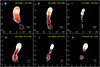 |
Fig. 1. Naturally weighted CLEAN images of FSRQ 1928+738 at 1.55, 4.15, 7.65, 15.2, 23.9, and 43.1 GHz, respectively. For each image, contours start at the 5σ image rms level and increase by a factor of 21/2. Physical scales are indicated in each map. Axis scales are in milliarcseconds. The blue ellipse in the top-left corner of each map is the synthesized beam. |
At a frequency of 1.6 GHz, the image displays an extended jet covering radial distances down to approximately 40 mas followed by an isolated feature at around 60 mas. This is consistent with previous VLBA observations at a similar frequency (1.4 GHz) by Pushkarev et al. (2017). The jet structure gradually becomes compact as the observing frequency increases, whereas the overall morphology remains broadly the same. Beyond the core region, the jet emission is dominated by an isolated feature at ≈5 mas. This feature remains distinctly visible even at 43 GHz, owing to its flat spectrum. We note that this feature is distinguishable from the core at all frequencies and can be identified via “modelfit”, even at the lowest resolution at 1.6 GHz (see Sect. 3.2).
It has been previously reported that the 1928+738 jet exhibits a curvature (see Eckart et al. 1985; Hummel et al. 1992; Roos et al. 1993; Homan et al. 2001, 2009; Kun et al. 2014; Roland et al. 2015). Figure 1 shows a result consistent with the reported curvature. The jet extends to the southeast with an approximate position angle (PA) of 160°, down to the bright feature at ≈5 mas. Then, the jet direction gradually turns toward the southwest – the farthest structure at 1.6 GHz has a PA of ∼195°. This behavior has been interpreted as a consequence of jet precession (Roos et al. 1993; Kun et al. 2014; Roland et al. 2015) or a helical jet structure (Hummel et al. 1992; Cheng et al. 2018). Homan et al. (2001, 2009) have suggested that the variation of the PA may result from jet collimation. We note that the origin of the jet curvature is beyond the scope of this work. Nevertheless, we had to consider the possibility that the viewing angle may not be constant, even at the smallest scales (see Raiteri et al. 2017; Readhead et al. 2021). We discuss this issue in Sect. 3.6.
3.2. Core identification, core shift, image alignment
The emission from the inner regions of AGN jets is usually optically thick because of synchrotron self-absorption and free-free absorption. Thus, the radio core is usually assumed to be a photosphere, that is, a region where the optical depth of the jet plasma reaches unity (Blandford & Königl 1979; Konigl 1981). We used a standard model-fitting routine, the Difmap task “modelfit”. After calibration and imaging, the visibility data at each frequency and each epoch was fitted with a set of circular Gaussian components. At any frequency, we identified the most upstream component as the core. The minimum resolvable size of Gaussian components is approximately 10 μas, assuming signal-to-noise ratios of several thousand (Lobanov 2005). We note that the cores of 1928+738 appear to be unresolved even at the highest resolution, yielding a compactness of θcore ≲ 10 μas at any given frequency.
The absorption mechanism depends on the observing frequency (e.g., Rybicki & Lightman 1979; Levinson et al. 1995) and so does the location of the core (e.g., Marcaide & Shapiro 1984; Lobanov 1998; Hirotani 2005). Thus, the higher the observing frequency, the closer is the core to the central black hole – the “core-shift”. The opacity effect thereby prevents the usage of the core as a common reference point when combining multifrequency data. Alignment of the jet images at different frequencies should be preceded by a precise measurement of the relative positions of the chromatic cores Δzc(ν1, ν2) = zc(ν1)−zc(ν2), where zc is the distance of the core from the black hole and ν2 > ν1. For this reason, we analyzed the core-shift in the 1928+738 jet before proceeding to the analysis of jet geometry and kinematics.
We used the “self-referencing” method, which is based on a 2D cross correlation of optically thin jet structures a few milliarcseconds away from the core (see Croke & Gabuzda 2008; O’Sullivan & Gabuzda 2009; Sokolovsky et al. 2011; Pushkarev et al. 2012; Fromm et al. 2013, 2015; Pushkarev et al. 2019; Park et al. 2021, for details). To enable an accurate comparison, we reconstructed the jet images at 1−24 GHz listed in Table 1 (see also, Figs. 1a–e), which were obtained simultaneously. For each frequency pair, the images were adjusted to have the same (u, v)-range and convolved with the same circular beam. Likewise, the pixel sizes were chosen to be identical. From the subsequent cross correlation, we determined the core-shift vector for the given frequency pair. We followed the convention (e.g., Fromm et al. 2013; Kutkin et al. 2014), to assume the uncertainties of the core-shift magnitude to be 1/20 of the convolved beam. We list all core-shifts thus derived in Table 4.
Core-shift measurements for each pair of frequencies.
At each frequency, we computed the core position with respect to the one at the highest frequency. The relative positions are presented in Fig. 2. A systematic decrease with increasing frequency is obvious in the figure. We describe the data with a quasi-reciprocal function, zc ∝ ν−1/kz (Blandford & Königl 1979; Konigl 1981), where the value of kz is determined by the magnetic field and electron density distribution along the jet. The special case kz = 1 corresponds to the case of synchrotron self-absorption dominated by nuclear opacity in a conical jet with energy equipartition. We performed a least-square fit using the function  , where Δzc(ν, 24) is the core position at frequency ν with respect to the one at 24 GHz. The best-fit parameter values are Ω = 2.21 ± 0.15 and kz = 1.87 ± 0.48 (see Fig. 2). The best-fit shows a reduced chi-square value χ2/d.o.f. = 1.38. Within the errors, the best-fit value of kz is marginally consistent with unity. Extrapolation of the best-fit line to higher frequencies is highly uncertain, so we assumed that the core-shift of the 24 GHz core is negligible, Δzc(ν, 24)≈0, even for ν → ∞.
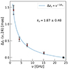 |
Fig. 2. Relative core positions of the 1928+738 jet as a function of frequency with respect to the 24 GHz core. The solid line shows the best-fit power-law function |
All data for the 1928+738 jet presented in this paper have been corrected for core-shift. A deeper analysis of the core-shift will be presented in a forthcoming paper, with a wider frequency coverage and a denser sampling of the observing frequency.
3.3. Possible limb brightening
We restored the jet images using circular beams with diameters corresponding to the geometric mean of the major axis and minor axis of the synthesized beams. This image reconstruction step removes distortion related to the beam shapes. A constant PA is usually adopted to describe the direction of a jet (e.g., Nakahara et al. 2018, 2019, 2020; Hada et al. 2018; Park et al. 2021); however, the jet of 1928+738 is curved. We therefore defined a jet axis by determining the locations of intensity maxima in the image plane (see Pushkarev et al. 2017; Kovalev et al. 2020; Okino et al. 2022). Using polar coordinates with the core as the center point, we measured the jet intensity profile along the azimuthal direction at multiple radii. At first glance, the jet appeared to have a single ridge; however, we found that the concentric intensity profile of the jet can only be described with two Gaussian functions in several cases, especially at 24 GHz. In Fig. 3, we present three examples of such profiles. We note that limb brightening in 1928+738 has not been reported before, probably due to the lower angular resolution and limited sensitivity of previous observations (e.g., VLBA 15 GHz image of Pushkarev et al. 2017). We plan to explore the limb brightening structure in the 1928+738 jet with future observations of higher angular resolution and higher sensitivity (Yi et al., in prep.).
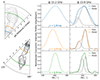 |
Fig. 3. Examples of jet intensity profile along the azimuthal direction. Left: two of our VLBA maps in polar coordinates, convolved with circular beams. The black solid and gray dashed contours represent the 24 GHz and 15 GHz images, respectively. The 15 GHz image has been rotated 180° to ease the presentation. Right: three concentric jet intensity profiles obtained at different angular distances z from the origin of the jet (represented by different colors). The solid and dotted lines denote the intensities at 24 GHz and 15 GHz, respectively. All profiles have been normalized to the unit maximum. |
3.4. Jet width profile
The jet radius R (i.e., the half width) scales with distance from the black hole, z, as R ∝ zm. The power-law index m is close to unity in the case of a classical conical jet, while m < 1 is expected for collimated jets (e.g., Asada & Nakamura 2012; Hada et al. 2018; Park et al. 2021). The images of 1928+738 (Fig. 1) allowed us to analyze the radius of its jet over a wide range of spatial scales.
We obtained transverse slices along the jet in one-third steps of the restoring beam size. We measured the full width half maximum (FWHM) of each slice and subtracted the beam FWHM in squares (deconvolution). The FWHM is measured by fitting the intensity profile with a Gaussian function. Whenever a single Gaussian function cannot describe the profile well, a double Gaussian is used. In those cases, we used the distance between the outer half-maximum points as a measure of the jet width (Hada et al. 2013, 2016; Park et al. 2021). We considered the measurements to be valid only when (i) adjacent distance bins are smoothly connected and (ii) the peak intensity of the slice exceeds 14 times the image rms level. The first few measurements, starting at the center point, were strongly affected by the core brightness, and we therefore discarded the distance bins out to 1.5 times the beam size away from the core. In this paper, we define the jet radius R as one-half of the deconvolved FWHM and use it as an indicator of the jet width. The uncertainties of the jet radii are assumed to be one-tenth of the beam sizes (see Park et al. 2021, for details). In this way, we could derive the jet radii covering distances from ∼0.8 mas to ∼40 mas. We present the jet radius as a function of distance from the black hole in Fig. 4. In general, the jet radii from different frequencies and different angular resolutions are consistent with each other, within errors (1σ confidence intervals), at given distance bins.
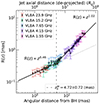 |
Fig. 4. Jet radius profile as a function of distance z from the black hole. The distance is displayed in units of Rg (top axis) and milliarcsecond (bottom axis). Error bars represent ±1σ uncertainties. The solid line represents the best-fit broken power-law model. The dotted line represents an extrapolation of the inner part of the best-fit model. The vertical dashed line indicates the location of the break in the jet width profile, |

We modeled the jet radius as function of distance with a broken power law, meaning in log space
 (1)
(1)
where  is the location of the break point, m1, 2 are the slopes, and b is a constant offset. This function describes the jet profile well over the full range of distances from the black hole. The best-fit profile has
  ) mas, with R ∝ z0.46 ± 0.10 (i.e., parabolic shape) and R ∝ z1.02 ± 0.03 (i.e., conical shape), before and after the break point, respectively.
Our fit is based on the assumption that the input errors solely depend on the beam size. Although our broken power-law model apparently fits the data well (see the solid line in Fig. 4), the goodness of the fit should be compared with a single power-law model quantitatively. We used the Bayesian information criterion (BIC), defined as BIC ≡ −2lnℒmax + klnN. Here, ℒmax is the maximum likelihood of a model, k is the number of free parameters, and N is the number of data points. Adopting the standard assumption of Gaussian errors, BIC = χ2 + klnN. The BIC of our best-fit broken power-law model is smaller than the BIC of the best-fit single power-law model by ΔBIC ≈ 34. Accordingly, a broken power-law model is strongly favored statistically, indicating a robust discovery of the jet collimation break (JCB) in FSRQ 1928+738.
3.5. Jet velocity field
We constrained the jet velocity field of FSRQ 1928+738 over the entire region inside and outside the JCB. We measured the proper motions of distinctive structures. As previously reported (e.g., Eckart et al. 1985), the brightness distribution of the jet is modeled well with a set of circular Gaussian components at all frequencies (see Sect. 3.2). We hereafter refer to the modelfit components as “knots”. For our kinematic analysis, we cross-identified and traced knots across different epochs. We used multi-epoch monitoring data from the KaVA Q-band, MOJAVE U-band, and the Astrogeo X- and S-bands, respectively (see Sect. 2). We note that we did not attempt cross-band identification of knots. The proper motion μz (in mas yr−1) and the corresponding apparent speed βapp(≡vapp/c) of each knot feature were derived by fitting their radial distance z with time. We detected proper motions at distances between ∼0.3 and ∼20 mas from the black hole. We provide the details for our modelfit analysis in Appendix A.
We assumed that the observed proper motions reflect the bulk motion of the jet flow (e.g., Lister et al. 2009; Nakamura & Asada 2013), given the continuous acceleration and deceleration profiles observed in various data across different frequencies and observing periods. However, it is noteworthy that the observed speeds, based on the modelfit analysis, may not always correspond to the bulk jet speeds. Instead, they may represent pattern speeds caused by, for example, jet instabilities (e.g., Hardee 2000) or stationary shocks.
We detected significant outward motions for most (22 out of 25) of the knots we traced. For three knots, the proper motion was not significantly different from zero, so we did not include them in our analysis. We then converted the apparent speed βapp of each knot into the intrinsic speed β = βapp/(sin θv + βappcosθv) and derived the bulk Lorentz factor  by adopting a viewing angle of θv = 13.2° (see Sect. 3.6). In Fig. 5, we present the radial profile of the bulk Lorentz factor. Interestingly, a systematic increase and a subsequent decrease of Γ are clearly visible in the velocity field, with a peak approximately at 5 mas. This indicates that the bulk jet is gradually accelerated in the inner region within a distance of ≈5 mas and decelerated at larger distances. The peak Γmax ≈ 10, calculated from the maximum observed speed βapp = 7.2, is broadly consistent with previous measurements by Lister et al. (2019) and Kun et al. (2014). We fit a broken power law to the Γ profile in the same way that we did for the jet radius R(z). During the fitting process, we noted that X3, one of the X-band knots, is an outlier that may not be associated with the underlying bulk flows, and we excluded it from the fit (this is discussed in Appendix B). We found a clear division into an inner and an outer velocity field, with Γ ∝ z0.46 ± 0.08 and Γ ∝ z−0.26 ± 0.25, connected at the break point
  mas.
mas.
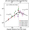 |
Fig. 5. Bulk Lorentz factor as a function of distance z from the black hole. The distance is displayed in units of Rg (top axis) and milliarcsecond (bottom axis). Colors indicate observations at different bands from various monitoring programs. Error bars represent ±1σ uncertainties. The solid line represents the best-fit broken power-law model. One of the knots traced at the X-band (X3), marked by an empty colored cross, is an outlier from the general relation. The vertical dashed line indicates the location of the transition point of the jet kinematics, |

Due to the limited range of distances in the jet of 1928+738 (less than one order of magnitude), the outer velocity field was poorly constrained. Nonetheless, the best fit describes the Γ profile well, with χ2/d.o.f. = 1.15. Moreover, we note that the outer trend of the jet deceleration is in good agreement with the slow jet speed on arcsecond (and kiloparsec) scales, which can be inferred from VLA/MERLIN observations (see Appendix C). We could therefore conclude that we discovered a distinct transition in the jet acceleration profile, a jet acceleration break, in FSRQ 1928+738.
The discovery of the jet acceleration and deceleration also implies the large dynamic range in the velocity of 1928+738 jet. However, the effectiveness of β and Γ in demonstrating the jet speed is limited to the non-relativistic regime (v ≪ c) and the relativistic regime (v → c), respectively. Thus, we hereafter use Γβ as a proxy for the bulk speed, which can represent both regimes.
3.6. Doppler factor and viewing angle
The motion of jet components toward the observer at relativistic speeds results in a boosting of the observed flux densities and a reduction of observed timescales. Beaming effects scale with the Doppler factor δ ≡ [Γ(1 − βcosθv)]−1. In this section, we analyze our KaVA 43 GHz monitoring data and estimate the variability Doppler factor for 1928+738.
In our KaVA 43 GHz images, we cross-identified four knots labeled Q1, Q2, Q3, and Q4 in order of increasing distance from the core. Their locations in a total intensity map and their light curves are presented in Fig. 6. Thanks to its high cadence, our KaVA monitoring enabled us to use an approach suggested by Jorstad et al. (2005, 2017) for deriving the Doppler factor. This approach relies on the evolution of modelfit parameters (i.e., flux, position, and size) of knots. We also refer the reader to Weaver et al. (2022).
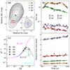 |
Fig. 6. Results of the KaVA 43 GHz monitoring. (a) Zoom-in view of the upstream region of the KaVA 43 GHz image in Fig. 1. The isolated jet feature at ≈5 mas is embedded in the bottom right of the plot. The four knots identified via the modelfit analysis are marked on the map. (b) Flux density and the displacements of the knots as functions of time. Exponential fits to the flux density data and linear fits to the motions are shown as continuous lines. (c) Relativistic beaming factor δ3 − α as a function of Γβ and assuming a spectral index of α = −0.5. We show our data along three theoretical lines corresponding to different values of θv. |
We estimated the uncertainties of the modelfit parameter values following the methods suggested by Lister et al. (2009) and Fomalont et al. (1999). We first considered a typical calibration error of 10−15% in the flux density. The positional uncertainty was set to one-fifth of the beam size, with the ratio of beam size and peak-to-noise ratio added in quadrature. In case of very compact and bright knots, these uncertainties were reduced by a factor of two. For the uncertainty in angular size, σa, we adopted the empirical scaling relation between size and brightness temperature Tb of Jorstad et al. (2017),
 (2)
(2)
where Tb is in units of Kelvin, the flux S is in units of Jansky, and the size a is in units of milliarcsecond.
We modeled the light curve of each knot as a sequence of an exponential rise and a subsequent exponential decay (Valtaoja et al. 1999; Hovatta et al. 2009):
 (3)
(3)
where So is the peak flux, tmax is the time of peak flux, and τrise and τdec denote the rise and decay timescales, respectively. We found that the brightest knot, Q1, experienced exponential flaring (i.e., rise and decay) twice during the observing period. One complete flare was also found in the second brightest knot, Q2. The remaining two knots only showed exponential decays. The exponential fits to the light curves are illustrated in Fig. 6b. The observed timescales are related to the intrinsic ones through τobs ≡ τint/δ. We identified the variability timescale τdec of a given knot with the light-travel time across the knot, which is valid as long as the flux decay is caused by radiative cooling. Under this assumption, the variability Doppler factor δ can be expressed as
![Mathematical equation: $$ \begin{aligned} \delta = 25.3\ \frac{(a \ [\mathrm{mas^{-1}}]) \ (D_{\rm L} \ [\mathrm{Gpc^{-1}}])}{(\tau _{\rm dec} \ [\mathrm{yr^{-1}}]) \ (1+z)}, \end{aligned} $$](/articles/aa/full_html/2024/08/aa49790-24/aa49790-24-eq12.gif) (4)
(4)
where a is the knot size (FWHM) and DL is the luminosity distance. This approach allowed us to compute the Doppler factors of the four individual knots. In addition, Eq. (4) is free from commonly used but highly idealized assumptions, such as energy equipartition between the radiating particles and the magnetic field or the viewing angle satisfying sin θc = 1/Γ. For our calculations, we used the knot sizes measured at times of maximum knot brightness (Casadio et al. 2015, 2019).
By combining the variability Doppler factor δ and the apparent speed βapp of each knot, we could infer the variability Lorentz factor Γvar and viewing angle θv from
 (5)
(5)
The results of our KaVA 43 GHz analysis are summarized in Table 5, which shows the values of the mean radial distance ⟨z⟩, the angular size a, the flux decaying timescale τdec, the Doppler factor δ, the Lorentz factor Γvar, and the jet viewing angle θv derived for each of the four knots. The uncertainties of δ, Γvar, and θv were estimated by means of standard error propagation.
Kinematics and physical parameters of the KaVA 43 GHz jet features.
Unfortunately, the analysis of knot Q1 appears rather unreliable. The exponential fits to the light curve do not constrain the decay timescales in a meaningful way, resulting in τdec = (0.98 ± 1.81) yr and τdec = (0.42 ± 0.60) yr for the first and second flare, respectively, meaning we had to disregard the fit results for our analysis (see, e.g., Weaver et al. 2022). Instead, we applied the empirical relation τdec = 1.3 × τrise (Valtaoja et al. 1999), which provides τdec = 0.68 ± 0.09 yr and leads to the values for δ, Γvar, and θv listed in Table 5.
The 1928+738 jet is characterized by mild variability, which indicates a relatively large viewing angle. Notably, we found an initial increase and subsequent decrease of the Doppler factor δ along the knots from Q1 to Q4, which presumably resulted from jet acceleration. This implies a specific brightness evolution since relativistic beaming scales with a factor δ3 − α, where α is the spectral index defined by Iν ∝ να. In Fig. 6, the beaming factor for the case α = −0.5 is displayed as a function of Γβ. The data points for the four knots match the theoretical line for θv = 13°. Moreover, we found that the viewing angle θv remains constant along the jet within errors. Indeed, our measurements provide observational evidence, for the first time, that jet collimation or acceleration (described in Sects. 3.4 and 3.5) is unrelated to changes in the viewing angle. We adopt the average value θv = 13.2° ±2.1° throughout this paper.
4. Discussion
In Fig. 7, we visualize the jet collimation and acceleration of 1928+738, by displaying the deprojected half-opening angle θj and Γβ as a function of deprojected distance from the black hole in units of Rg and parsec. The half-opening angle declines down to ≈1° at around 100 pc. Meanwhile, Γβ, which is assumed to represent the bulk jet speed, increases with distance and reaches its maximum, Γβ ∼ 10, likewise at ∼100 pc. Evidently, jet acceleration and collimation occur in the same region, the ACZ. Beyond the ACZ, one may expect the jet to decelerate slowly, with the opening angle θj remaining constant. Figure 7 shows that the data are consistent with this expectation. We identified the downstream end of the ACZ by independently measuring the locations of the jet collimation and acceleration breaks  and
and  (see Sects. 3.4 and 3.5). The two values are in good agreement; the shaded area in Fig. 7 denotes their average and the corresponding 1σ confidence interval, ⟨zb⟩=(5.6 ± 0.7)×106 Rg. In this section, we discuss the jet collimation and jet acceleration of 1928+738 separately.
 |
Fig. 7. Collimation and acceleration of the 1928+738 jet as a function of distance from the black hole. The distance is displayed in units of parsec (top axis) and Rg (bottom axis). Top: intrinsic half-opening angle θj as derived from the observed jet width profile. Bottom: Γβ calculated from the proper motions. The shaded area denotes the location where the ACZ terminates, ⟨zb⟩=(5.6 ± 0.7)×106 Rg. |
4.1. Jet collimation
A number of analytical and numerical studies (e.g., Komissarov et al. 2007; Lyubarsky 2009; Nakamura et al. 2018) have shown that external pressure pext is responsible for jet collimation. The external pressure profile pext ∝ z−κ needs to be sufficiently flat (i.e., κ ≦ 2) to collimate the jet (e.g., Komissarov et al. 2009). The source of pext is most likely the ambient medium confining the jet, which has been captured by the gravitational field of the black hole. Thus, the range of gravitational influence of the black hole in the center of 1928+738 is of particular interest.
The sphere of gravitational influence (SOI) can be defined as  , where σ* is the stellar velocity dispersion (Peebles 1972) in the center of the host galaxy. Assuming that the stars and the ionized gas around the black hole (e.g., [O III]λ5007 line-emitting gas) are bound by the same gravitational potential (e.g., Nelson & Whittle 1996; Boroson 2003), σ[O III] can be used as a proxy for σ*. We adopted σ[O III] = 166 km s−1 for 1928+738 (Marziani et al. 1996; Bian & Zhao 2004), which gave us RSOI ≈ 3.3 × 10⁶ Rg. However, one may expect σ[O III] > σ* due to the contribution of non-gravitational motion (e.g., turbulence) to the gas dynamics (e.g., Greene & Ho 2005; Woo et al. 2006; Bennert et al. 2018; Sexton et al. 2021). Overall, our value for RSOI can be considered a rough estimate and/or a lower limit. An additional estimate for σ* is provided by the empirical M• − σ* relation (e.g., Kormendy & Ho 2013). In this case, RSOI is solely determined by the black hole mass, which for 1928+738 is M• ≈ 3.7 × 10⁸ M⊙ and thus RSOI ≈ 2.1 × 10⁶ Rg.
Both estimates of RSOI show an order-of-magnitude consistency with ⟨zb⟩, the location where the ACZ terminates in 1928+738. This is the first time that such a coincidence has been reported for a quasar (Okino et al. 2022; Burd et al. 2022), although such a scaling has been found in a few nearby radio galaxies. Asada & Nakamura (2012) suggested that the JCB in M 87 occurs near the SOI, which is characterized by the Bondi radius  (where cs is the sound speed of X-ray emitting hot gas). Likewise, in NGC 6251, the JCB is found at approximately RSOI (Tseng et al. 2016). The remarkable similarity of the situation in 1928+738 with the one in low-luminosity AGNs suggests that an interplay between the jet and external medium could be a fundamental requirement for AGN jet collimation. In the case of low-luminosity AGNs, non-relativistic winds from the hot accretion flow (e.g., Yuan et al. 2015) within the Bondi radius and/or SOI have been suggested to serve as the external confining medium (e.g., Nakamura et al. 2018; Park et al. 2019b). Likewise, such winds are a likely candidate for medium surrounding the jet in 1928+738. If so, it is necessary to investigate the wind properties within the ACZ of this quasar for which a cold5 accretion flow is expected (e.g., Crenshaw et al. 2003). Future VLBI polarimetric observations for Faraday rotation may provide more information about the ambient medium (Yi et al., in prep.).
4.2. Jet acceleration
In Fig. 7, we observed that the 1928+738 jet gradually accelerates to relativistic speeds over a range of several million Rg, which is consistent with the basic characteristics of MHD acceleration (e.g., Vlahakis & Königl 2004; Beskin 2010). The jet acceleration is accompanied by jet collimation, as the MHD jet acceleration model predicts. Such models also predict that collimation and acceleration of a jet stop at the same distance from the black hole – which is exactly what we observed in 1928+738 and is what has been observed in M 87 (e.g., Asada & Nakamura 2012; Asada et al. 2014), NGC 315 (Park et al. 2021), and 1H 0323+342 (Hada et al. 2018). We note that possible co-spatial jet acceleration and collimation has also been reported for a few other radio galaxies (NGC 6251; Sudou et al. 2000, Cygnus A; Boccardi et al. 2016, and NGC 4261; Yan et al. 2023). However, 1928+738 is the first case where an extended ACZ has been discovered in the jet of an FSRQ.
The concurrent acceleration and collimation can be interpreted as a signature of “differential collimation” (also known as the magnetic nozzle effect; e.g., Camenzind 1987; Li et al. 1992; Begelman & Li 1994). The mechanism can cause the poloidal magnetic field lines to have both an inner concentration and an outer divergence. This field configuration can act as a nozzle, effectively converting the Poynting flux into kinetic energy (see Komissarov 2011; Nakamura & Asada 2013). The efficient jet acceleration through the energy conversion gives rise to “linear acceleration”, as the bulk Lorentz factor Γ increases linearly with the jet radius (Γ ∝ R; e.g., Beskin & Nokhrina 2006; Tchekhovskoy et al. 2008; Lyubarsky 2009). Again, this matches our observations of 1928+738, and the collimation and acceleration profiles (see Sects. 3.4 and 3.5) are consistent with Γ ∝ R(∝z0.46) out to ⟨zb⟩≈5.6 × 10⁶ Rg.
In order to make jet acceleration through differential bunching of poloidal magnetic fields possible, the field lines must be able to communicate laterally (e.g., Zakamska et al. 2008; Tchekhovskoy et al. 2009). This lateral causal connection is maintained if the opening angle of the jet is narrower than that of the Mach cone, meaning  (Komissarov et al. 2009), where σm is the magnetization parameter (i.e., the ratio of the Poynting flux and matter energy flux) of the jet. The degree of jet magnetization is still an open problem though, but we could infer the lower limit from the simultaneous jet collimation and acceleration. Given that the jet needs to convert the electromagnetic energy into kinetic energy, the jet also needs to be magnetized in the ACZ. Thus, we assumed σm ≳ 1; the jet is at least moderately magnetized. We found that the value of Γθj is approximately 0.1−0.2 along the ACZ of the 1928+738 jet. This implies that the jet satisfies the Mach cone condition. We therefore identified the magnetic nozzle effect as the most likely mechanism for the acceleration and collimation of the 1928+738 jet. Interestingly, the value of Γθj = 0.1 − 0.2 derived from the ACZ of the 1928+738 jet is in good agreement with values for a variety of AGN jets, mostly in distant blazars (Clausen-Brown et al. 2013; Jorstad et al. 2017; Pushkarev et al. 2017). The jet ACZs in those sources are expected to have been challenging to resolve with previous VLBI observations. The consistency in the Γθj values between 1928+738 and the distant blazars, despite the different spatial scales probed, may suggest that the jets possess causal connections over a broad distance range. Furthermore, the termination of the ACZ may not be strongly related to these causal connections but to other factors, such as the environment surrounding the jets, as discussed in Sect. 4.1.
4.3. Comparison with other AGN sources
In the following, we compare the jet collimation and acceleration profiles of 1928+738 with those of M 87, NGC 315, and 1H 0323+342. Though they represent different AGN types, the jet profiles of other sources in the 103 − 105 Rg may provide important information for interpreting the results we find for 1928+738. We note we only included the jet collimation profile of 1H 0323+342 because its jet acceleration profile is relatively unclear. The overall results are illustrated in Fig. 8.
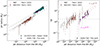 |
Fig. 8. Comparison with other AGN sources. Left: comparison of the jet radius of 1928+738 in the collimation zone as a function of deprojected distance from the black hole with M 87, NGC 315 and 1H 0323+342 in units of Rg. For 1H 0323+342, M• = 2 × 10⁷ M⊙ and θv = 8° are assumed in this plot. The M 87 data have been compiled from numerous previous studies (see Nakamura et al. 2018, and references therein). The data for NGC 315 and 1H 0323+342 are from Park et al. (2021) and Hada et al. (2018), respectively. Their best-fit power-law scaling relations R ∝ z0.58 are indicated by dashed lines. Right: comparison of the jet velocity field (Γβ) in the acceleration zone as a function of deprojected distance from the black hole in units of Rg of 1928+738 with those of M 87 and NGC 315. The M 87 data have been compiled from numerous previous studies (see Park et al. 2019a, and references therein), and the NGC 315 data are from Park et al. (2021). The black dashed horizontal line indicates Γ = 2 for illustration. The best-fit jet acceleration profiles of NGC 315 (Park et al. 2021) and 1928+738 (Sect. 3.5) are also presented with colored dashed lines for comparison. |
4.3.1. Jet collimation
In Fig. 8, the radii of the jets in the collimation zone as a function of distance are compared in the left panel. Whereas all jets show similar parabolic geometries, the jet radius profile of 1928+738 is clearly offset from those of M 87 (Asada & Nakamura 2012; Doeleman et al. 2012; Hada et al. 2013; Nakamura & Asada 2013; Akiyama et al. 2015; Nakamura et al. 2018) and NGC 315 (Park et al. 2021). The profiles of 1928+738 and 1H 0323+342 (Hada et al. 2018), however, agree within errors. There is a clear dichotomy: The jets of 1928+738 and 1H 0323+342 are systematically broader than those of M 87 and NGC 315 at any given distance. The best-fit power-law profiles of NGC 315 and 1H 0323+342 both show R ∝ z0.58 (see Park et al. 2021; Hada et al. 2018, respectively). Adopting the same power-law index for 1928+738 for comparison (instead of the observed one from Sect. 3.4), we found a difference in the jet width by a factor of approximately four (≈0.6 dex).
One explanation for the broad jet of 1928+738 could be a relatively high internal pressure, pjet, near the black hole. The high initial pjet then results in a relatively large volume (i.e., a broad jet) governed by the pressure equilibrium between the jet and its surroundings (Zakamska et al. 2008). We note that a similar scenario was examined by Narayan et al. (2022). Their recent simulation at scales of z ≦ 100 Rg suggested that a larger magnetic flux near the central black hole produces a broader jet. If these hold, the magnetic pressure and/or magnetic flux near the black hole of 1928+738 might explain its jet width. Nonetheless, we could not find observational evidence for such a high magnetic flux in 1928+738. Zamaninasab et al. (2014) inferred the magnetic flux threading parsec-scale jets, which is the same as the magnetic flux threading the black hole by the flux-freezing approximation. The inferred magnetic flux of 1928+738 appears to be comparable to those of M 87 and other radio galaxies. If this is true, this may indicate that the jets themselves are somewhat similar to each other. The difference in the jet width may then be a consequence of the external environment. Indeed, radio-loud quasars (and NLS1s) are widely believed to have an environment distinct from radio galaxies, including radiation-driven winds and strong radiation pressure (e.g., Ohsuga & Mineshige 2011; Dorodnitsyn et al. 2016; Davis & Tchekhovskoy 2020). We note that broad jets have also been found in other FSRQs, such as 1633+382 (also known as 4C 38.41; Algaba et al. 2019) and 3C 273 (Okino et al. 2022), although further studies are needed for a quantitative comparison.
4.3.2. Jet acceleration
We present the jet velocity fields Γβ of 1928+738, M 87 (Biretta et al. 1995, 1999; Cheung et al. 2007; Ly et al. 2007; Giroletti et al. 2012; Meyer et al. 2013; Asada et al. 2014; Hada et al. 2016, 2017; Mertens et al. 2016; Kim et al. 2018; Walker et al. 2018; Park et al. 2019a), and NGC 315 (Park et al. 2021) in the right panel of Fig. 8. Although it is difficult to compare the complex Γβ profiles in depth, the 1928+738 jet again seems to deviate from the other sources: The velocity profile appears to be shifted outward and/or downward, resulting in a relatively low speed at a given distance.
An inward extrapolation of the acceleration profile Γ ∝ z0.46 suggests that the jet speed remains v ≪ c at distances z ≲ 105 Rg. The bulk jet velocity of 1928+738 becomes mildly relativistic (e.g., Γ ≳ 2) at distances of a few 105 Rg, which is much later than is the case for the other AGNs or as expected theoretically (e.g., McKinney 2006; Penna et al. 2013; Nakamura et al. 2018). Given that linear acceleration is only valid when the jet is sufficiently fast (e.g., Beskin & Nokhrina 2006; Komissarov et al. 2007, 2009), one may expect the early-phase acceleration to not be very efficient. If this is the case, the early-phase acceleration profile of the 1928+738 jet in the non-relativistic or sub-relativistic regime could be similar to what has been observed in M 876 (Γ ∝ z0.16, Park et al. 2019a) or NGC 3157 (Γ ∝ z0.30, Park et al. 2021). The jet kinematics at distances of 104 − 105 Rg might then reveal how the bulk speed of the 1928+738 jet remains slow at such far a distance. Moreover, velocity measurements using more densely sampled observations at higher angular resolutions are known to report faster motions in case of the M 87 jet (see e.g., Walker et al. 2008, for related discussions). Likewise, it may be necessary to perform a jet kinematic analysis using data with a higher resolution and observing cadence to obtain a more accurate velocity field for 1928+738. We leave this exploration to future work.
5. Summary
We have investigated the collimation and acceleration of the jet of a nearby FSRQ, 1928+738. We compiled multifrequency and multi-epoch VLBA data from various archives and reported the observational results. We also performed complementary monitoring observations with KaVA to study the variability of the jet. We summarize our main results below:
-
We obtained multifrequency VLBI images of the 1928+738 jet at various spatial scales, showing an extended jet down to ≈40 mas from the radio core. Based on a 2D cross-correlation analysis of optically thin jet structures, we measured the frequency-dependent location of the radio core, which follows zc ∝ ν−1/kz, where kz = 1.87 ± 0.48. The core-shift measurements allowed us to accurately align the jet collimation and acceleration profiles obtained from the multifrequency data.
-
We extensively investigated the jet radius profile, covering the distance range from ∼0.8 mas to ∼40 mas. We discovered that the jet geometry transits from a parabolic shape (R ∝ z0.46 ± 0.10) to a conical shape (R ∝ z1.02 ± 0.03) at a distance of
 mas. We also performed a complementary kinematic analysis. We found that the bulk Lorentz factor Γ, too, transits from acceleration (Γ ∝ z0.46 ± 0.08) to deceleration (Γ ∝ z−0.26 ± 0.25) at a distance of
  mas. By combining the collimation profile and the jet velocity field, we discovered that the collimation and acceleration of the jet occur in the same region.
 -
We studied the jet variability using our monitoring observations with KaVA at 43 GHz. We derived the variability Doppler factors δvar and the viewing angle θv for four knots at distances of ≲5 mas, which have been reliably cross-identified throughout the ≈2 yr of observation. We found that the viewing angle remains constant along the jet, within errors, with an average value of ⟨θ⟩ = 13.2°.
-
Adopting the viewing angle θv = 13.2° and a black hole mass M• ≈ 3 × 10⁸ M⊙, the deprojected distance to the downstream end of the ACZ is ⟨zb⟩≈5.6 × 10⁶ Rg. This is similar to the sphere of gravitational influence of the black hole in the center of 1928+738. This implies that the physical extent of the ACZ in the 1928+738 jet is governed by the gravitational field of the black hole. The jet might be collimated by winds from accretion flows.
-
We found that the jet gradually accelerates to highly relativistic speeds, with Γ ∼ 10, over a distance of several million Rg. We found a linear relation between the bulk Lorentz factor and jet radius, Γ ∝ R, in agreement with theoretical expectations for MHD acceleration and collimation of highly magnetized jets. We conclude that the jet is accelerated through the magnetic nozzle effect, efficiently converting the Poynting flux into kinetic energy.
-
We compared the jet collimation and acceleration of 1928+738 with other AGNs. The jet of 1928+738 is broader at a given distance than those of M 87 and NGC 315. We enumerate two possibilities for this: (i) the magnetic pressure and/or magnetic flux near the black hole of 1928+738 might be substantially higher than in the other sources or (ii) the broad jet might be a consequence of the distinctive external environment of the 1928+738 jet compared to the jets from radio galaxies. In addition, we found that the bulk jet speed of 1928+738 is relatively slow at a given distance. This implies that the early-phase acceleration of the jet is much flatter than Γ ∝ z0.46 at distances ≤105 Rg.
We finally remark that 1928+738 is the first radio-loud quasar and the fourth AGN (following M 87, 1H 0323+342, and NGC 315) for which there is robust evidence of a genuine ACZ, characterized by the co-spatial jet acceleration and collimation over a large distance range, in line with predictions from the MHD jet acceleration. We plan to conduct a deeper analysis on core-shift, limb-brightening, and polarization characteristics of the 1928+738 jet, through forthcoming observations with superior angular resolution and enhanced sensitivity.
Korean VLBI Network, which consists of three 21 m telescopes in Korea.
VLBI Exploration of Radio Astrometry, which consists of four 20 m telescopes in Japan.
Cold accretion flows are presumed to be characteristic for accretion at a relatively high Eddington ratio Ṁ/ṀEdd ≳ 1% (e.g., Ghisellini et al. 2011; Heckman & Best 2014). We note that the Eddington ratio of 1928+738 has been found to be ≳60% (e.g., Park & Trippe 2017).
Mertens et al. (2016) actually suggested a more complicated evolution, including a transition from Γ ∝ z0.56 to Γ ∝ z0.16. However, the authors used only the upper envelope of the proper motion data point cloud to derive the profiles (see Sect. 6.2 of Park et al. 2019a, for related discussions).
We note, however, that Ricci et al. (2022) suggested an efficient acceleration, describing Γ as a hyperbolic tangent function of z.
Acknowledgments
We thank the anonymous referee for constructive and detailed comments, which were helpful to improve the manuscript. We acknowledge the use of data from the Astrogeo Center database maintained by Leonid Petrov, Yuri Kovalev and Yuzhu Cui. This research has made use of data from the MOJAVE database that is maintained by the MOJAVE team (Lister et al. 2018). The VLBA is an instrument of the National Radio Astronomy Observatory. The National Radio Astronomy Observatory is a facility of the National Science Foundation operated by Associated Universities, Inc. This work is made use of the East Asian VLBI Network (EAVN), which is operated under cooperative agreement by National Astronomical Observatory of Japan (NAOJ), Korea Astronomy and Space Science Institute (KASI), with the operational support by Kagoshima University (for the operation of VERA Iriki antenna). We acknowledge financial support from the National Research Foundation of Korea (NRF) through grant 2022R1F1A1075115. This work was supported by the BK21 FOUR program through National Research Foundation of Korea (NRF) under Ministry of Education (Kyung Hee University, Human Education Team for the Next Generation of Space Exploration). M.N. is supported by JSPS KAKENHI Grant Number JP24K07100.
References
- Akiyama, K., Lu, R.-S., Fish, V. L., et al. 2015, ApJ, 807, 150 [NASA ADS] [CrossRef] [Google Scholar]
- Akiyama, K., Asada, K., Fish, V., et al. 2018, Galaxies, 6, 15 [NASA ADS] [CrossRef] [Google Scholar]
- Algaba, J. C., Rani, B., Lee, S. S., et al. 2019, ApJ, 886, 85 [NASA ADS] [CrossRef] [Google Scholar]
- An, T., Sohn, B. W., & Imai, H. 2018, Nat. Astron., 2, 118 [Google Scholar]
- Asada, K., & Nakamura, M. 2012, ApJ, 745, L28 [NASA ADS] [CrossRef] [Google Scholar]
- Asada, K., Nakamura, M., Doi, A., Nagai, H., & Inoue, M. 2014, ApJ, 781, L2 [Google Scholar]
- Begelman, M. C., & Li, Z.-Y. 1994, ApJ, 426, 269 [NASA ADS] [CrossRef] [Google Scholar]
- Bennert, V. N., Loveland, D., Donohue, E., et al. 2018, MNRAS, 481, 138 [NASA ADS] [CrossRef] [Google Scholar]
- Beskin, V. S. 2010, Phys. Usp., 53, 1199 [NASA ADS] [CrossRef] [Google Scholar]
- Beskin, V. S., & Nokhrina, E. E. 2006, MNRAS, 367, 375 [Google Scholar]
- Bian, W., & Zhao, Y. 2004, MNRAS, 347, 607 [NASA ADS] [CrossRef] [Google Scholar]
- Biretta, J. A., Zhou, F., & Owen, F. N. 1995, ApJ, 447, 582 [NASA ADS] [CrossRef] [Google Scholar]
- Biretta, J. A., Sparks, W. B., & Macchetto, F. 1999, ApJ, 520, 621 [NASA ADS] [CrossRef] [Google Scholar]
- Blandford, R. D., & Königl, A. 1979, ApJ, 232, 34 [Google Scholar]
- Blandford, R. D., & Payne, D. G. 1982, MNRAS, 199, 883 [CrossRef] [Google Scholar]
- Blandford, R. D., & Znajek, R. L. 1977, MNRAS, 179, 433 [NASA ADS] [CrossRef] [Google Scholar]
- Blandford, R., Meier, D., & Readhead, A. 2019, ARA&A, 57, 467 [NASA ADS] [CrossRef] [Google Scholar]
- Boccardi, B., Krichbaum, T. P., Bach, U., et al. 2016, A&A, 585, A33 [NASA ADS] [CrossRef] [EDP Sciences] [Google Scholar]
- Boccardi, B., Migliori, G., Grandi, P., et al. 2019, A&A, 627, A89 [NASA ADS] [CrossRef] [EDP Sciences] [Google Scholar]
- Boccardi, B., Perucho, M., Casadio, C., et al. 2021, A&A, 647, A67 [NASA ADS] [CrossRef] [EDP Sciences] [Google Scholar]
- Boroson, T. A. 2003, ApJ, 585, 647 [NASA ADS] [CrossRef] [Google Scholar]
- Burd, P. R., Kadler, M., Mannheim, K., et al. 2022, A&A, 660, A1 [NASA ADS] [CrossRef] [EDP Sciences] [Google Scholar]
- Camenzind, M. 1987, A&A, 184, 341 [NASA ADS] [Google Scholar]
- Casadio, C., Gómez, J. L., Jorstad, S. G., et al. 2015, ApJ, 813, 51 [Google Scholar]
- Casadio, C., Marscher, A. P., Jorstad, S. G., et al. 2019, A&A, 622, A158 [NASA ADS] [CrossRef] [EDP Sciences] [Google Scholar]
- Cheng, X. P., An, T., Hong, X. Y., et al. 2018, ApJS, 234, 17 [NASA ADS] [CrossRef] [Google Scholar]
- Cheung, C. C., Harris, D. E., & Stawarz, Ł. 2007, ApJ, 663, L65 [NASA ADS] [CrossRef] [Google Scholar]
- Cho, I., Zhao, G.-Y., Kawashima, T., et al. 2022, ApJ, 926, 108 [NASA ADS] [CrossRef] [Google Scholar]
- Clausen-Brown, E., Savolainen, T., Pushkarev, A. B., Kovalev, Y. Y., & Zensus, J. A. 2013, A&A, 558, A144 [NASA ADS] [CrossRef] [EDP Sciences] [Google Scholar]
- Condon, J., Darling, J., Kovalev, Y. Y., & Petrov, L. 2011, arXiv e-prints [arXiv:1110.6252] [Google Scholar]
- Crenshaw, D. M., Kraemer, S. B., & George, I. M. 2003, ARA&A, 41, 117 [NASA ADS] [CrossRef] [Google Scholar]
- Croke, S. M., & Gabuzda, D. C. 2008, MNRAS, 386, 619 [CrossRef] [Google Scholar]
- Cui, Y., Hada, K., Kawashima, T., et al. 2023, Nature, 621, 711 [NASA ADS] [CrossRef] [Google Scholar]
- Davis, S. W., & Tchekhovskoy, A. 2020, ARA&A, 58, 407 [Google Scholar]
- Doeleman, S. S., Fish, V. L., Schenck, D. E., et al. 2012, Science, 338, 355 [NASA ADS] [CrossRef] [Google Scholar]
- Dorodnitsyn, A., Kallman, T., & Proga, D. 2016, ApJ, 819, 115 [NASA ADS] [CrossRef] [Google Scholar]
- Eckart, A., Witzel, A., Biermann, P., et al. 1985, ApJ, 296, L23 [NASA ADS] [CrossRef] [Google Scholar]
- Fanaroff, B. L., & Riley, J. M. 1974, MNRAS, 167, 31P [Google Scholar]
- Fomalont, E. B., Goss, W. M., Beasley, A. J., & Chatterjee, S. 1999, AJ, 117, 3025 [NASA ADS] [CrossRef] [Google Scholar]
- Fromm, C. M., Ros, E., Perucho, M., et al. 2013, A&A, 551, A32 [NASA ADS] [CrossRef] [EDP Sciences] [Google Scholar]
- Fromm, C. M., Perucho, M., Ros, E., Savolainen, T., & Zensus, J. A. 2015, A&A, 576, A43 [NASA ADS] [CrossRef] [EDP Sciences] [Google Scholar]
- Ghisellini, G., Tavecchio, F., Foschini, L., & Ghirlanda, G. 2011, MNRAS, 414, 2674 [NASA ADS] [CrossRef] [Google Scholar]
- Giovannini, G., Savolainen, T., Orienti, M., et al. 2018, Nat. Astron., 2, 472 [Google Scholar]
- Giroletti, M., Hada, K., Giovannini, G., et al. 2012, A&A, 538, L10 [NASA ADS] [CrossRef] [EDP Sciences] [Google Scholar]
- Greene, J. E., & Ho, L. C. 2005, ApJ, 627, 721 [NASA ADS] [CrossRef] [Google Scholar]
- Greisen, E. W. 2003, in AIPS, the VLA, and the VLBA, ed. A. Heck, Astrophys. Space Sci. Lib., 285, 109 [Google Scholar]
- Hada, K. 2019, Galaxies, 8, 1 [NASA ADS] [CrossRef] [Google Scholar]
- Hada, K., Doi, A., Nagai, H., et al. 2013, ApJ, 779, 6 [NASA ADS] [CrossRef] [Google Scholar]
- Hada, K., Kino, M., Doi, A., et al. 2016, ApJ, 817, 131 [Google Scholar]
- Hada, K., Park, J. H., Kino, M., et al. 2017, PASJ, 69, 71 [NASA ADS] [CrossRef] [Google Scholar]
- Hada, K., Doi, A., Wajima, K., et al. 2018, ApJ, 860, 141 [NASA ADS] [CrossRef] [Google Scholar]
- Hada, K., Niinuma, K., Sitarek, J., Spingola, C., & Hirano, A. 2020, ApJ, 901, 2 [NASA ADS] [CrossRef] [Google Scholar]
- Hardee, P. E. 2000, ApJ, 533, 176 [Google Scholar]
- Heckman, T. M., & Best, P. N. 2014, ARA&A, 52, 589 [Google Scholar]
- Hirotani, K. 2005, ApJ, 619, 73 [Google Scholar]
- Homan, D. C., Ojha, R., Wardle, J. F. C., et al. 2001, ApJ, 549, 840 [NASA ADS] [CrossRef] [Google Scholar]
- Homan, D. C., Kadler, M., Kellermann, K. I., et al. 2009, ApJ, 706, 1253 [NASA ADS] [CrossRef] [Google Scholar]
- Homan, D. C., Lister, M. L., Kovalev, Y. Y., et al. 2015, ApJ, 798, 134 [Google Scholar]
- Hovatta, T., Valtaoja, E., Tornikoski, M., & Lähteenmäki, A. 2009, A&A, 494, 527 [CrossRef] [EDP Sciences] [Google Scholar]
- Hummel, C. A., Schalinski, C. J., Krichbaum, T. P., et al. 1992, A&A, 257, 489 [NASA ADS] [Google Scholar]
- Johnston, K. J., Simon, R. S., Eckart, A., et al. 1987, ApJ, 313, L85 [NASA ADS] [CrossRef] [Google Scholar]
- Jorstad, S. G., Marscher, A. P., Lister, M. L., et al. 2005, AJ, 130, 1418 [Google Scholar]
- Jorstad, S. G., Marscher, A. P., Morozova, D. A., et al. 2017, ApJ, 846, 98 [Google Scholar]
- Junor, W., Biretta, J. A., & Livio, M. 1999, Nature, 401, 891 [NASA ADS] [CrossRef] [Google Scholar]
- Kellermann, K. I., Lister, M. L., Homan, D. C., et al. 2004, ApJ, 609, 539 [NASA ADS] [CrossRef] [Google Scholar]
- Kim, J. Y., Krichbaum, T. P., Lu, R. S., et al. 2018, A&A, 616, A188 [NASA ADS] [CrossRef] [EDP Sciences] [Google Scholar]
- Kino, M., Wajima, K., Kawakatu, N., et al. 2018, ApJ, 864, 118 [NASA ADS] [CrossRef] [Google Scholar]
- Komissarov, S. S. 2011, Mem. Soc. Astron. It., 82, 95 [NASA ADS] [Google Scholar]
- Komissarov, S. S., Barkov, M. V., Vlahakis, N., & Königl, A. 2007, MNRAS, 380, 51 [Google Scholar]
- Komissarov, S. S., Vlahakis, N., Königl, A., & Barkov, M. V. 2009, MNRAS, 394, 1182 [NASA ADS] [CrossRef] [Google Scholar]
- Konigl, A. 1981, ApJ, 243, 700 [Google Scholar]
- Kormendy, J., & Ho, L. C. 2013, ARA&A, 51, 511 [Google Scholar]
- Kovalev, Y. Y., Petrov, L., Fomalont, E. B., & Gordon, D. 2007, AJ, 133, 1236 [NASA ADS] [CrossRef] [Google Scholar]
- Kovalev, Y. Y., Pushkarev, A. B., Nokhrina, E. E., et al. 2020, MNRAS, 495, 3576 [NASA ADS] [CrossRef] [Google Scholar]
- Kun, E., Gabányi, K. É., Karouzos, M., Britzen, S., & Gergely, L. Á. 2014, MNRAS, 445, 1370 [CrossRef] [Google Scholar]
- Kutkin, A. M., Sokolovsky, K. V., Lisakov, M. M., et al. 2014, MNRAS, 437, 3396 [Google Scholar]
- Lähteenmäki, A., & Valtaoja, E. 1999, ApJ, 521, 493 [Google Scholar]
- Lawrence, C. R., Pearson, T. J., Readhead, A. C. S., & Unwin, S. C. 1986, AJ, 91, 494 [NASA ADS] [CrossRef] [Google Scholar]
- Lee, S.-S., Oh, C. S., Roh, D.-G., et al. 2015a, J. Korean Astron. Soc., 48, 125 [NASA ADS] [CrossRef] [Google Scholar]
- Lee, S.-S., Byun, D.-Y., Oh, C. S., et al. 2015b, J. Korean Astron. Soc., 48, 229 [NASA ADS] [CrossRef] [Google Scholar]
- Lee, T., Trippe, S., Kino, M., et al. 2019, MNRAS, 486, 2412 [NASA ADS] [CrossRef] [Google Scholar]
- Levinson, A., Laor, A., & Vermeulen, R. C. 1995, ApJ, 448, 589 [NASA ADS] [CrossRef] [Google Scholar]
- Li, Z.-Y., Chiueh, T., & Begelman, M. C. 1992, ApJ, 394, 459 [NASA ADS] [CrossRef] [Google Scholar]
- Liodakis, I., Hovatta, T., Huppenkothen, D., et al. 2018, ApJ, 866, 137 [Google Scholar]
- Lister, M. L., Cohen, M. H., Homan, D. C., et al. 2009, AJ, 138, 1874 [NASA ADS] [CrossRef] [Google Scholar]
- Lister, M. L., Aller, M. F., Aller, H. D., et al. 2018, ApJS, 234, 12 [CrossRef] [Google Scholar]
- Lister, M. L., Homan, D. C., Hovatta, T., et al. 2019, ApJ, 874, 43 [NASA ADS] [CrossRef] [Google Scholar]
- Lister, M. L., Homan, D. C., Kellermann, K. I., et al. 2021, ApJ, 923, 30 [NASA ADS] [CrossRef] [Google Scholar]
- Lobanov, A. P. 1998, A&A, 330, 79 [NASA ADS] [Google Scholar]
- Lobanov, A. P. 2005, arXiv e-prints [arXiv:astro-ph/0503225] [Google Scholar]
- Ly, C., Walker, R. C., & Junor, W. 2007, ApJ, 660, 200 [NASA ADS] [CrossRef] [Google Scholar]
- Lyubarsky, Y. 2009, ApJ, 698, 1570 [NASA ADS] [CrossRef] [Google Scholar]
- Marcaide, J. M., & Shapiro, I. I. 1984, ApJ, 276, 56 [Google Scholar]
- Marscher, A. P., Jorstad, S. G., D’Arcangelo, F. D., et al. 2008, Nature, 452, 966 [Google Scholar]
- Marziani, P., Sulentic, J. W., Dultzin-Hacyan, D., Calvani, M., & Moles, M. 1996, ApJS, 104, 37 [Google Scholar]
- McKinney, J. C. 2006, MNRAS, 368, 1561 [NASA ADS] [CrossRef] [Google Scholar]
- Meier, D. L., Koide, S., & Uchida, Y. 2001, Science, 291, 84 [Google Scholar]
- Mertens, F., Lobanov, A. P., Walker, R. C., & Hardee, P. E. 2016, A&A, 595, A54 [NASA ADS] [CrossRef] [EDP Sciences] [Google Scholar]
- Meyer, E. T., Sparks, W. B., Biretta, J. A., et al. 2013, ApJ, 774, L21 [NASA ADS] [CrossRef] [Google Scholar]
- Nakahara, S., Doi, A., Murata, Y., et al. 2018, ApJ, 854, 148 [NASA ADS] [CrossRef] [Google Scholar]
- Nakahara, S., Doi, A., Murata, Y., et al. 2019, ApJ, 878, 61 [NASA ADS] [CrossRef] [Google Scholar]
- Nakahara, S., Doi, A., Murata, Y., et al. 2020, AJ, 159, 14 [Google Scholar]
- Nakamura, M., & Asada, K. 2013, ApJ, 775, 118 [NASA ADS] [CrossRef] [Google Scholar]
- Nakamura, M., Asada, K., Hada, K., et al. 2018, ApJ, 868, 146 [Google Scholar]
- Narayan, R., Chael, A., Chatterjee, K., Ricarte, A., & Curd, B. 2022, MNRAS, 511, 3795 [NASA ADS] [CrossRef] [Google Scholar]
- Nelson, C. H., & Whittle, M. 1996, ApJ, 465, 96 [NASA ADS] [CrossRef] [Google Scholar]
- Niinuma, K., Lee, S.-S., Kino, M., et al. 2014, PASJ, 66, 103 [NASA ADS] [CrossRef] [Google Scholar]
- Oh, J., Trippe, S., Kang, S., et al. 2015, J. Korean Astron. Soc., 48, 299 [NASA ADS] [CrossRef] [Google Scholar]
- Ohsuga, K., & Mineshige, S. 2011, ApJ, 736, 2 [NASA ADS] [CrossRef] [Google Scholar]
- Okino, H., Akiyama, K., Asada, K., et al. 2022, ApJ, 940, 65 [NASA ADS] [CrossRef] [Google Scholar]
- O’Sullivan, S. P., & Gabuzda, D. C. 2009, MNRAS, 400, 26 [Google Scholar]
- Park, J., & Trippe, S. 2017, ApJ, 834, 157 [CrossRef] [Google Scholar]
- Park, J., Hada, K., Kino, M., et al. 2019a, ApJ, 887, 147 [Google Scholar]
- Park, J., Hada, K., Kino, M., et al. 2019b, ApJ, 871, 257 [Google Scholar]
- Park, J., Hada, K., Nakamura, M., et al. 2021, ApJ, 909, 76 [Google Scholar]
- Peebles, P. J. E. 1972, ApJ, 178, 371 [NASA ADS] [CrossRef] [Google Scholar]
- Penna, R. F., Narayan, R., & Sądowski, A. 2013, MNRAS, 436, 3741 [Google Scholar]
- Petrov, L. 2021, AJ, 161, 14 [Google Scholar]
- Petrov, L., Kovalev, Y. Y., Fomalont, E. B., & Gordon, D. 2006, AJ, 131, 1872 [NASA ADS] [CrossRef] [Google Scholar]
- Petrov, L., Kovalev, Y. Y., Fomalont, E. B., & Gordon, D. 2008, AJ, 136, 580 [NASA ADS] [CrossRef] [Google Scholar]
- Pushkarev, A. B., & Kovalev, Y. Y. 2012, A&A, 544, A34 [NASA ADS] [CrossRef] [EDP Sciences] [Google Scholar]
- Pushkarev, A. B., Hovatta, T., Kovalev, Y. Y., et al. 2012, A&A, 545, A113 [NASA ADS] [CrossRef] [EDP Sciences] [Google Scholar]
- Pushkarev, A. B., Kovalev, Y. Y., Lister, M. L., & Savolainen, T. 2017, MNRAS, 468, 4992 [Google Scholar]
- Pushkarev, A. B., Butuzova, M. S., Kovalev, Y. Y., & Hovatta, T. 2019, MNRAS, 482, 2336 [NASA ADS] [CrossRef] [Google Scholar]
- Raiteri, C. M., Villata, M., Acosta-Pulido, J. A., et al. 2017, Nature, 552, 374 [NASA ADS] [CrossRef] [Google Scholar]
- Readhead, A. C. S., Ravi, V., Liodakis, I., et al. 2021, ApJ, 907, 61 [NASA ADS] [CrossRef] [Google Scholar]
- Ricci, L., Boccardi, B., Nokhrina, E., et al. 2022, A&A, 664, A166 [NASA ADS] [CrossRef] [EDP Sciences] [Google Scholar]
- Roland, J., Britzen, S., Kun, E., et al. 2015, A&A, 578, A86 [NASA ADS] [CrossRef] [EDP Sciences] [Google Scholar]
- Roos, N., Kaastra, J. S., & Hummel, C. A. 1993, ApJ, 409, 130 [NASA ADS] [CrossRef] [Google Scholar]
- Rybicki, G. B., & Lightman, A. P. 1979, Radiative Processes in Astrophysics (New York: Wiley) [Google Scholar]
- Sexton, R. O., Matzko, W., Darden, N., Canalizo, G., & Gorjian, V. 2021, MNRAS, 500, 2871 [Google Scholar]
- Shepherd, M. C. 1997, in Astronomical Data Analysis Software and Systems VI, eds. G. Hunt, & H. Payne, ASP Conf. Ser., 125, 77 [Google Scholar]
- Sokolovsky, K. V., Kovalev, Y. Y., Pushkarev, A. B., & Lobanov, A. P. 2011, A&A, 532, A38 [CrossRef] [EDP Sciences] [Google Scholar]
- Sudou, H., Taniguchi, Y., Ohyama, Y., et al. 2000, PASJ, 52, 989 [NASA ADS] [CrossRef] [Google Scholar]
- Tchekhovskoy, A., McKinney, J. C., & Narayan, R. 2008, MNRAS, 388, 551 [NASA ADS] [CrossRef] [Google Scholar]
- Tchekhovskoy, A., McKinney, J. C., & Narayan, R. 2009, ApJ, 699, 1789 [NASA ADS] [CrossRef] [Google Scholar]
- Traianou, E., Krichbaum, T. P., Boccardi, B., et al. 2020, A&A, 634, A112 [NASA ADS] [CrossRef] [EDP Sciences] [Google Scholar]
- Tseng, C.-Y., Asada, K., Nakamura, M., et al. 2016, ApJ, 833, 288 [NASA ADS] [CrossRef] [Google Scholar]
- Urry, C. M., & Padovani, P. 1995, PASP, 107, 803 [NASA ADS] [CrossRef] [Google Scholar]
- Valtaoja, E., Lähteenmäki, A., Teräsranta, H., & Lainela, M. 1999, ApJS, 120, 95 [NASA ADS] [CrossRef] [Google Scholar]
- Vlahakis, N. 2015, Theory of Relativistic Jets, in The Formation and Disruption of Black Hole Jets, eds. I. Contopoulos, D. Gabuzda, & N. Kylafis, 414, 177 [NASA ADS] [CrossRef] [Google Scholar]
- Vlahakis, N., & Königl, A. 2004, ApJ, 605, 656 [Google Scholar]
- Wajima, K., Hagiwara, Y., An, T., et al. 2016, in Frontiers in Radio Astronomy and FAST Early Sciences Symposium 2015, eds. L. Qain, & D. Li, ASP Conf. Ser., 502, 81 [Google Scholar]
- Wajima, K., Kino, M., & Kawakatu, N. 2020, ApJ, 895, 35 [Google Scholar]
- Walker, R. C., Ly, C., Junor, W., & Hardee, P. J. 2008, J. Phys. Conf. Ser., 131, 012053 [Google Scholar]
- Walker, R. C., Hardee, P. E., Davies, F. B., Ly, C., & Junor, W. 2018, ApJ, 855, 128 [Google Scholar]
- Weaver, Z. R., Jorstad, S. G., Marscher, A. P., et al. 2022, ApJS, 260, 12 [NASA ADS] [CrossRef] [Google Scholar]
- Woo, J.-H., Treu, T., Malkan, M. A., & Blandford, R. D. 2006, ApJ, 645, 900 [NASA ADS] [CrossRef] [Google Scholar]
- Yan, X., Lu, R.-S., Jiang, W., Krichbaum, T. P., & Shen, Z.-Q. 2023, ApJ, 957, 32 [NASA ADS] [CrossRef] [Google Scholar]
- Yuan, F., Gan, Z., Narayan, R., et al. 2015, ApJ, 804, 101 [NASA ADS] [CrossRef] [Google Scholar]
- Zakamska, N. L., Begelman, M. C., & Blandford, R. D. 2008, ApJ, 679, 990 [Google Scholar]
- Zamaninasab, M., Clausen-Brown, E., Savolainen, T., & Tchekhovskoy, A. 2014, Nature, 510, 126 [Google Scholar]
Appendix A: Modelfit jet kinematics
We provide here additional information about our kinematic analysis. The Astrogeo X- and S-band data sets required more careful analysis compared to the MOJAVE and KaVA data sets, due to their non-uniform angular resolution and cadence. Thus, we only analyzed the knots located at least about one (averaged) beam away from the core in order to avoid misidentifications. In total, we cross-identified eight knots at the X-band and three at the S-band. The knots detected at the X-band are labeled X1, X2, and so on until X8, and the knots detected at the S-band are labeled S1, S2, and S3. We also cross-identified ten knots over time from the MOJAVE U band data set and labeled them U1, U2, U3, and so on until U10. We present the knot locations within stacked Astrogeo and MOJAVE images in Figure A.1 and Figure A.2, respectively. We note that the CLEAN images were stacked after convolution with the average circular beams. The motion of the knots with time is presented along the maps. In Table A.1 and Table A.2, the mean radial distance ⟨z⟩, angular proper motion (in mas/yr), and apparent speed (in units of light speed) of individual knots are listed.
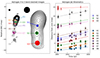 |
Fig. A.1. Results of the Astrogeo modelfit jet kinematics. Left: Stacked images of naturally weighted CLEAN maps of 1928+738 at X- and S-bands from the Astrogeo program. The averaged circular beams with sizes of 1.57 mas and 5.43 mas, respectively, are shown in the top left of each contour map. The jet components are labeled individually. Right: Distance from the core as a function of time (data points) for all Astrogeo knots detected at ≲8.6 GHz with linear fits (straight lines) overlaid. The different markers are used to distinguish observing frequencies. |
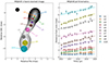 |
Fig. A.2. Results of the MOJAVE modelfit jet kinematics. Left: Stacked image of naturally weighted CLEAN maps of 1928+738 at the U-band from the MOJAVE program. The averaged circular beam with a size of 0.63 mas is shown in the top-left corner. Jet components are labeled individually. Right: Distance from the core as a function of time (data points) for the MOJAVE knots detected at 15 GHz with linear fits (straight lines) overlaid. |
Astrogeo jet kinematics.
MOJAVE jet kinematics.
Appendix B: Outlier identification
As described in Section 3.5, we modeled the bulk Lorentz factor of 1928+738 as a function of distance with a broken power-law function. However, one of the knots was identified as an outlier and excluded from the fit by doing the following: We generated multiple bootstrap samples, fit a broken power-law model to each sample, and then examined the stability of the best-fit model parameters, including the power-law index, the break location  , and the maximum Lorentz factor Γmax. Since the number of knots is small, each bootstrap sample includes all data points except one. In Figure B.1, we show the best-fit parameter values for each bootstrap sample. Knot X3 is an obvious outlier.
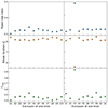 |
Fig. B.1. Best-fit parameter values. From top to bottom: Power-law index, break location |

Appendix C: Slow jet speeds and the counter-jet
In this appendix, we discuss the counter-jet of 1928+738 and its detectability. As introduced in Section 1, it is evident that 1928+738 shows a two-sided morphology on arcsecond scales (e.g., Johnston et al. 1987; Hummel et al. 1992). The difference in the brightness of the two-sided jets at the same distance can be explained by the result of Doppler boosting and de-boosting, assuming that they are intrinsically the same. The jet-to-counter-jet brightness ratio (BR) is directly related to the bulk flow speed β and the viewing angle θv via
 (C.1)
(C.1)
where Ijet and Icjet denote the intensities of the jet and counter-jet at the same distance, and α is the spectral index. Adopting BR ≈ 10, which is measured by a MERLIN 408 MHz observation at 2 arcsec (Hummel et al. 1992), we could infer the jet speed at such a far distance. We present the result in Figure C.1 as a form of the bulk Lorentz factor Γ together with a part of the velocity field in Figure 5, where it shows a gradual deceleration. The jet speed inferred from the BR shows a good agreement with other data points obtained from the kinematics analysis. We found that the broken power-law fit of the velocity field (Section 3.5) is not greatly affected by the inclusion of this new data point (see Figure C.1). This may imply that there is indeed a jet deceleration, and it is maintained down to over 109 Rg; however, it is not used for our main analysis, owing to the large distance gap (i.e., approximately two orders of magnitude).
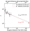 |
Fig. C.1. Bulk Lorentz factor as a function of distance z from the black hole. The distance is displayed in units of Rg (top axis) and milliarcsecond (bottom axis). The data includes the decelerating part in Figure 5 (gray data points) and the result inferred from the MERLIN observation at 408 MHz (red data point; see text). Error bars represent ±1σ uncertainties. The black dashed line represents the best-fit broken power-law model in Figure 5, and the red one represents the model obtained by including the red data. |
On the other hand, there is little evidence of the counter-jet in VLBI observations on (sub-)mas scales (see Figure 1). Nevertheless, the non-detection also allowed us to constrain the jet speed at the nearest distance of the proper motion. As described in Section 3.6, the slowest motion is detected approximately at 0.35 mas from 43 GHz KaVA observations. At that location, we can estimate BR ≳ 435 from the 43 GHz KaVA image (see Figure 1) by adopting Icjet ≲ 5σrms. We could infer the lower limit to the jet speed Γ ≳ 1.67 for the case α = −0.5, which agrees well with the slowest speed detected (i.e., Γ = 1.76). This supports the robustness of our main analysis. We also note that a slightly different value of α between -1 and 0 does not affect our conclusion. We plan to have a more robust analysis on the counter-jet through future multifrequency observations with higher angular resolution and higher sensitivity (Yi et al., in prep.).
All Tables
All Figures
|
Fig. 1. Naturally weighted CLEAN images of FSRQ 1928+738 at 1.55, 4.15, 7.65, 15.2, 23.9, and 43.1 GHz, respectively. For each image, contours start at the 5σ image rms level and increase by a factor of 21/2. Physical scales are indicated in each map. Axis scales are in milliarcseconds. The blue ellipse in the top-left corner of each map is the synthesized beam. |
| In the text | |
|
Fig. 2. Relative core positions of the 1928+738 jet as a function of frequency with respect to the 24 GHz core. The solid line shows the best-fit power-law function |
| In the text | |
|
Fig. 3. Examples of jet intensity profile along the azimuthal direction. Left: two of our VLBA maps in polar coordinates, convolved with circular beams. The black solid and gray dashed contours represent the 24 GHz and 15 GHz images, respectively. The 15 GHz image has been rotated 180° to ease the presentation. Right: three concentric jet intensity profiles obtained at different angular distances z from the origin of the jet (represented by different colors). The solid and dotted lines denote the intensities at 24 GHz and 15 GHz, respectively. All profiles have been normalized to the unit maximum. |
| In the text | |
|
Fig. 4. Jet radius profile as a function of distance z from the black hole. The distance is displayed in units of Rg (top axis) and milliarcsecond (bottom axis). Error bars represent ±1σ uncertainties. The solid line represents the best-fit broken power-law model. The dotted line represents an extrapolation of the inner part of the best-fit model. The vertical dashed line indicates the location of the break in the jet width profile, |
| In the text | |
|
Fig. 5. Bulk Lorentz factor as a function of distance z from the black hole. The distance is displayed in units of Rg (top axis) and milliarcsecond (bottom axis). Colors indicate observations at different bands from various monitoring programs. Error bars represent ±1σ uncertainties. The solid line represents the best-fit broken power-law model. One of the knots traced at the X-band (X3), marked by an empty colored cross, is an outlier from the general relation. The vertical dashed line indicates the location of the transition point of the jet kinematics, |
| In the text | |
|
Fig. 6. Results of the KaVA 43 GHz monitoring. (a) Zoom-in view of the upstream region of the KaVA 43 GHz image in Fig. 1. The isolated jet feature at ≈5 mas is embedded in the bottom right of the plot. The four knots identified via the modelfit analysis are marked on the map. (b) Flux density and the displacements of the knots as functions of time. Exponential fits to the flux density data and linear fits to the motions are shown as continuous lines. (c) Relativistic beaming factor δ3 − α as a function of Γβ and assuming a spectral index of α = −0.5. We show our data along three theoretical lines corresponding to different values of θv. |
| In the text | |
|
Fig. 7. Collimation and acceleration of the 1928+738 jet as a function of distance from the black hole. The distance is displayed in units of parsec (top axis) and Rg (bottom axis). Top: intrinsic half-opening angle θj as derived from the observed jet width profile. Bottom: Γβ calculated from the proper motions. The shaded area denotes the location where the ACZ terminates, ⟨zb⟩=(5.6 ± 0.7)×106 Rg. |
| In the text | |
|
Fig. 8. Comparison with other AGN sources. Left: comparison of the jet radius of 1928+738 in the collimation zone as a function of deprojected distance from the black hole with M 87, NGC 315 and 1H 0323+342 in units of Rg. For 1H 0323+342, M• = 2 × 10⁷ M⊙ and θv = 8° are assumed in this plot. The M 87 data have been compiled from numerous previous studies (see Nakamura et al. 2018, and references therein). The data for NGC 315 and 1H 0323+342 are from Park et al. (2021) and Hada et al. (2018), respectively. Their best-fit power-law scaling relations R ∝ z0.58 are indicated by dashed lines. Right: comparison of the jet velocity field (Γβ) in the acceleration zone as a function of deprojected distance from the black hole in units of Rg of 1928+738 with those of M 87 and NGC 315. The M 87 data have been compiled from numerous previous studies (see Park et al. 2019a, and references therein), and the NGC 315 data are from Park et al. (2021). The black dashed horizontal line indicates Γ = 2 for illustration. The best-fit jet acceleration profiles of NGC 315 (Park et al. 2021) and 1928+738 (Sect. 3.5) are also presented with colored dashed lines for comparison. |
| In the text | |
|
Fig. A.1. Results of the Astrogeo modelfit jet kinematics. Left: Stacked images of naturally weighted CLEAN maps of 1928+738 at X- and S-bands from the Astrogeo program. The averaged circular beams with sizes of 1.57 mas and 5.43 mas, respectively, are shown in the top left of each contour map. The jet components are labeled individually. Right: Distance from the core as a function of time (data points) for all Astrogeo knots detected at ≲8.6 GHz with linear fits (straight lines) overlaid. The different markers are used to distinguish observing frequencies. |
| In the text | |
|
Fig. A.2. Results of the MOJAVE modelfit jet kinematics. Left: Stacked image of naturally weighted CLEAN maps of 1928+738 at the U-band from the MOJAVE program. The averaged circular beam with a size of 0.63 mas is shown in the top-left corner. Jet components are labeled individually. Right: Distance from the core as a function of time (data points) for the MOJAVE knots detected at 15 GHz with linear fits (straight lines) overlaid. |
| In the text | |
|
Fig. B.1. Best-fit parameter values. From top to bottom: Power-law index, break location |
| In the text | |
|
Fig. C.1. Bulk Lorentz factor as a function of distance z from the black hole. The distance is displayed in units of Rg (top axis) and milliarcsecond (bottom axis). The data includes the decelerating part in Figure 5 (gray data points) and the result inferred from the MERLIN observation at 408 MHz (red data point; see text). Error bars represent ±1σ uncertainties. The black dashed line represents the best-fit broken power-law model in Figure 5, and the red one represents the model obtained by including the red data. |
| In the text | |
Current usage metrics show cumulative count of Article Views (full-text article views including HTML views, PDF and ePub downloads, according to the available data) and Abstracts Views on Vision4Press platform.
Data correspond to usage on the plateform after 2015. The current usage metrics is available 48-96 hours after online publication and is updated daily on week days.
Initial download of the metrics may take a while.