| Issue |
A&A
Volume 558, October 2013
|
|
|---|---|---|
| Article Number | A109 | |
| Number of page(s) | 13 | |
| Section | Planets and planetary systems | |
| DOI | https://doi.org/10.1051/0004-6361/201321690 | |
| Published online | 14 October 2013 | |
Theoretical models of planetary system formation: mass vs. semi-major axis
1
Physikalisches Institut & Center for Space and Habitability,
Universität Bern,
3012
Bern,
Switzerland
e-mail:
This email address is being protected from spambots. You need JavaScript enabled to view it.
; This email address is being protected from spambots. You need JavaScript enabled to view it.
; This email address is being protected from spambots. You need JavaScript enabled to view it.
; This email address is being protected from spambots. You need JavaScript enabled to view it.
; This email address is being protected from spambots. You need JavaScript enabled to view it.
; This email address is being protected from spambots. You need JavaScript enabled to view it.
2
Observatoire de Besançon, 41 avenue de l’Observatoire,
25000
Besançon,
France
e-mail:
This email address is being protected from spambots. You need JavaScript enabled to view it.
3
Max-Planck Institute for Astronomy, Königstuhl 17, 69117
Heidelberg,
Germany
e-mail:
This email address is being protected from spambots. You need JavaScript enabled to view it.
Received:
12
April
2013
Accepted:
8
July
2013
Abstract
Context. Planet formation models have been developed during the past years to try to reproduce what has been observed of both the solar system and the extrasolar planets. Some of these models have partially succeeded, but they focus on massive planets and, for the sake of simplicity, exclude planets belonging to planetary systems. However, more and more planets are now found in planetary systems. This tendency, which is a result of radial velocity, transit, and direct imaging surveys, seems to be even more pronounced for low-mass planets. These new observations require improving planet formation models, including new physics, and considering the formation of systems.
Aims. In a recent series of papers, we have presented some improvements in the physics of our models, focussing in particular on the internal structure of forming planets, and on the computation of the excitation state of planetesimals and their resulting accretion rate. In this paper, we focus on the concurrent effect of the formation of more than one planet in the same protoplanetary disc and show the effect, in terms of architecture and composition of this multiplicity.
Methods. We used an N-body calculation including collision detection to compute the orbital evolution of a planetary system. Moreover, we describe the effect of competition for accretion of gas and solids, as well as the effect of gravitational interactions between planets.
Results. We show that the masses and semi-major axes of planets are modified by both the effect of competition and gravitational interactions. We also present the effect of the assumed number of forming planets in the same system (a free parameter of the model), as well as the effect of the inclination and eccentricity damping. We find that the fraction of ejected planets increases from nearly 0 to 8% as we change the number of embryos we seed the system with from 2 to 20 planetary embryos. Moreover, our calculations show that, when considering planets more massive than ~5 M⊕, simulations with 10 or 20 planetary embryos statistically give the same results in terms of mass function and period distribution.
Key words: planets and satellites: formation / planets and satellites: composition / planetary systems
© ESO, 2013
1. Introduction
Since the pioneering discovery of 51 Peg b (Mayor & Queloz 1995), the first extrasolar planet orbiting a solar type star, the statistics of planetary observations have shown exponential growth. This tendency has been amplified during the past years by the growing number of planetary candidates discovered by Kepler (Borucki et al. 2011). One interesting feature in these planetary observations, which is a characteristic of both radial velocity and transit surveys, is that the number of planetary systems is also growing extremely rapidly (see e.g. Lovis et al. 2011; Mayor et al. 2011; Lissauer et al. 2011). Such planetary systems are very interesting for planet formation theory, since they can provide constraints on the processes acting during planet formation. For example, the presence of resonant systems seems to be very probably linked to migration during planet formation. On the other hand, from the theoretical point of view, and as we see in this paper, the formation of a planetary system is a problem significantly more difficult to solve than the formation of an isolated planet.
Indeed, the formation of a planetary system involves not only the formation process of the individual planets themselves, a process which is far from being fully understood for the moment, but also all the interactions between these planets. Among all these interactions, one can mention the following.
-
Growing planets, in particular when they are close to each other,are competitors for the accretion of solids and gas.
-
Planetesimal accretion can be strongly perturbed by the presence of neighbouring planets that can generate density waves of solids thanks to the excitation they produce in the random velocity of planetesimals (Guilera et al. 2010, 2011). Depending on the location of planets, the planet-mass ratio, the density profile of the disc, and the size of planetesimals, the accretion rate of planetesimals can be reduced or enhanced.
-
The formation of a planet in the wake of another one is strongly perturbed. This was shown in the case of the solar system (Alibert et al. 2005b) and the HD 69830 system (Alibert et al. 2006) using simplified models.
-
Gravitational interactions between forming planets modify their migration and may lead to mean-motion resonances systems.
-
Collisions between protoplanets, or ejections of some planets, are likely to occur during the whole formation phase.
-
Gap formation in a disc is modified when more than one planet is present. Moreover, the merging of two neighbouring gaps leads to modification of migration (see Masset & Snellgrove 2001).
-
When a planet forms a gap, the outer boundary of the gap may represent a place of very reduced type I migration, thus acting as a planet trap (Masset et al. 2006).
In a forthcoming series of papers, we intend to improve our planet formation models, in terms of both the physical and numerical treatments of some of the important processes involved in the formation of a system (migration, protoplanetary disc structure and evolution, and planet internal structure) and to include some of the aforementioned interaction effects. Improved disc models and planet internal structure models have been described in Mordasini et al. (2012a,b, M12a and M12b and Fortier et al. (2013, F13 and improved migration models are presented in Dittkrist et al. (in prep.). In this paper, we focus on the effect of forming more than one planet in the same protoplanetary disc. We present the numerical approach used to compute the gravitational interactions and collisions between planets, the treatment of the competition for solid accretion, and the differential effect of having more than one planet growing and migrating in the same disc. The interactions between forming planets, mediated through the gas component of the protoplanetary disc (a first planet modifying the protoplanetary disc – e.g. by gap formation or spiral wave generation – this leading to, e.g., a modified migration of a second planet), will be considered in another work, since it requires the development of new numerical models. As a consequence, although we consider populations of planets that are not fundamentally different from observed populations, our results should only be considered as a step toward a complete understanding of planetary population, and will likely be improved and modified in the future. The specific application of our models to the case of the solar system will be considered in a future paper, since the process of gap merging is likely to have played an important role in this case (see Walsh et al. 2011).
The paper is organized as follows. We present in Sect. 2 a summary of the most important physical features of our models, summarizing the work presented elsewhere (for details see M12a; M12b; F13). This section is presented for the sake of completeness, and can be skipped by readers having read the papers mentioned above. In Sect. 3, we describe the computation of the planet’s orbital evolution (including planet-planet gravitational interactions and disc-planet interactions) and collision detection. In Sect. 4, we present our treatment of the competition for the accretion of solids and gas. In Sect. 5 we present the results, considering both an example of ten-planet system formation models, and the results of planetary population synthesis, comparing the case where only one planet forms in the protoplanetary disc, and the case where multiple planets form. As we see later, the number of planets growing in the disc is a free parameter of the model, and we present in this paper the case where 1, 2, 5, 10, and 20 planetary embryos grow and migrate in the disc and discuss the sensitivity of the results to this number. Finally, in Sect. 6, we discuss our results and limitations and future developments of the models.
2. Formation model
The formation model consists of different modules, each of them computing one important class of physical processes involved during the formation of a planetary system. These modules are related to the protoplanetary disc structure and evolution (including both vertical and radial structure), the computation of the planetesimals’ dynamical properties and accretion rate, the planets’ internal structure, and the dynamical interactions between planets and between the disc and the planets. These different modules have already been described elsewhere (e.g. Alibert et al. 2005a, hereafter A05; M12a; M12b; F13).
2.1. Protoplanetary disc: gas phase
2.1.1. Vertical structure
The structure of protoplanetary discs is complex and different effects may be important. There could be irradiation and also the presence of a dead zone. In our model, the vertical disc structure is computed by solving the equations for hydrostatic equilibrium, energy conservation, and diffusion for the radiative flux (see A05; F13).
This calculation provides us with the vertically averaged viscosity as a function of
the surface density in the disc. In the models presented here, we assume that the local
viscosity is given by the Shakura-Sunyaev approximation (Shakura & Sunyaev 1973),  ,
where Cs is the local sound speed, Ω the Keplerian
frequency, and α a free parameter, taken to be 2 × 10⁻³ in
this paper.
,
where Cs is the local sound speed, Ω the Keplerian
frequency, and α a free parameter, taken to be 2 × 10⁻³ in
this paper.
2.1.2. Evolution
The evolution of the gas disc surface density is computed by solving the diffusion
equation: ![Mathematical equation: \begin{equation} {{\rm d} \Sigma \over {\rm d} t} = {3 \over r} {\partial \over \partial r } \left[ r^{1/2} {\partial \over \partial r} \tilde{\nu} \Sigma r^{1/2} \right] + \dot{\Sigma}_w(r) + \dot{Q}_{\rm planet}(r) \label{eqdiff}. \end{equation}](/articles/aa/full_html/2013/10/aa21690-13/aa21690-13-eq8.png) (1)Photoevaporation is
included using the model of Veras & Armitage
(2004):
(1)Photoevaporation is
included using the model of Veras & Armitage
(2004): 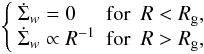 (2)where
Rg is usually taken to be 5 AU, and the total mass loss
due to photo-evaporation is a free parameter. The sink term
(2)where
Rg is usually taken to be 5 AU, and the total mass loss
due to photo-evaporation is a free parameter. The sink term
 is equal to the gas mass accreted by the forming planets. For every forming planet, gas
is removed from the protoplanetary disc in an annulus centred on the planet and with a
width equal to the planet’s Hill radius
is equal to the gas mass accreted by the forming planets. For every forming planet, gas
is removed from the protoplanetary disc in an annulus centred on the planet and with a
width equal to the planet’s Hill radius 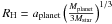 .
.
Equation 1 is solved on a grid that extends from the innermost radius of the disc to 1000 AU. At these two points, the surface density is constantly equal to nought. The innermost radius of the disc is of the order of 0.1 AU and is taken from observations (see Table 1 in Sect. 5.2).
2.2. Protoplanetary disc: solid phase
2.2.1. Planetesimal characteristics
In our model, we consider two kinds of planetesimals: rocky and icy. These two kinds of planetesimals differ by their physical properties, in particular by their mean density (3.2 g/cm3 for the former, 1 g/cm3 for the latter). Initially, the disc of rocky planetesimals extends from the innermost point in the disc (given by the fourth column of Table 1 in Sect. 5.2), to the initial location of the ice line, whereas the disc of icy planetesimals extends from the ice line to the outermost point in the simulation disc.
The location of the ice line is computed from the initial gas disc model, using the central temperature and pressure. The ice sublimation temperature we use depends on the total pressure. In our model, the location of the ice line does not evolve with time. In particular, no condensation of moist gas or sublimation of icy planetesimals is taken into account. Moreover, the location of the ice line being based on the central pressure and temperature, the ice line is supposed to be independent of the height in the disc. In reality the ice line is likely to be an “ice surface” whose location depends on the height inside the disc (see Min et al. 2011). We assume that all planetesimals have the same radius (of the order of 100 m) and that this radius does not evolve with time. The extension of our calculations towards a non-uniform and time-evolving planetesimal mass function will be the subject of future work. The assumed radius of the planetesimals has a strong effect on the resulting formation process of planetary systems. Increasing their radius to a few tens of kilometers severely decreases their accretion rate and the growth of planets. This effect was discussed in F13.
2.2.2. Planetesimal surface density and excitation
The eccentricity and inclination of planetesimals are important since they in part govern the accretion rate of solids and the ability of planets to grow. In the present paper, we follow the approach presented in F13 of computing the rms eccentricity and inclination of planetesimals as a result of excitation by planets and damping by gas drag. Since more than one planet form in the same disc, planetesimals excited by a planet can remain excited when they enter the feeding zone of another planet, modifying their capture probability1.
The dynamical state of the planetesimal disc is computed by solving differential equations that describe the evolution of the excitation and damping rates of their mean eccentricity and inclination. As pointed out in F13, the memory of the initial value of the planetesimals eccentricity and inclination can last for a non-negligible time. We assume here that the initial excitation state of planetesimals is the one resulting from the self-interaction between planetesimals alone (cold planetesimals initially). This corresponds to the assumption that planetary embryos (whose mass is 10-2 M⊕) appear instantaneously, as a result of, say, gas-solid interactions (e.g. Johansen et al. 2007).
2.3. Planetary growth and competition
2.3.1. Solid accretion rate
We start our calculation with a collection of low-mass embryos (mass
10-2 M⊕), which may accrete solids and gas,
and may migrate in the protoplanetary disc. The solid accretion rate of a given embryo
is computed following the approach described in F13, including the effect of the atmosphere, which enhances the cross-section.
The latter is parametrized by the embryo capture radius, the effective radius of the
planets for the accretion of planetesimals, which is computed using the results of Inaba & Ikoma (2003), and is given by the
following implicit equation: ![Mathematical equation: \begin{equation} \rpla = { 3 \rhogas (\rcap) \rcap \over 2 \rhopla } \left[ {\vrel^2 + { 2 G m (\rcap) \over \rcap } \over \vrel^2 + { 2 G m (\rcap) \over \rhill } } \right] , \end{equation}](/articles/aa/full_html/2013/10/aa21690-13/aa21690-13-eq16.png) (3)where
Rplanetesimals is the physical radius of the
planetesimals, ρgas is the density at a distance
Rcap from the planet centre,
m(Rcap) is the planetary mass inside the
sphere of radius Rcap centred on the planet’s centre, and
vrel is the relative velocity between the planet and the
planetesimals, which results from their excitation state. Tests have shown that the
capture radii obtained with these approximate formula are very close to the ones
obtained by computing the trajectory of planetesimals inside the planetary envelope (see
the method described in A05).
(3)where
Rplanetesimals is the physical radius of the
planetesimals, ρgas is the density at a distance
Rcap from the planet centre,
m(Rcap) is the planetary mass inside the
sphere of radius Rcap centred on the planet’s centre, and
vrel is the relative velocity between the planet and the
planetesimals, which results from their excitation state. Tests have shown that the
capture radii obtained with these approximate formula are very close to the ones
obtained by computing the trajectory of planetesimals inside the planetary envelope (see
the method described in A05).
2.3.2. Gas accretion
The accretion of gas by growing planets is the result of planetary contraction. This is computed by solving the internal structure equations for the planetary envelope, considering as energy source both the accretion energy of planetesimals and the compression work released by the contraction of the planetary envelope. The method is similar to the one presented in F13, to which the reader is referred to for more details. Note that we assume in this model that the dust opacity in the planetary envelope is reduced compared to interstellar values (see Pollack et al. 1996; Movshovitz et al. 2010). For the sake of simplicity and following the approach of Pollack et al. (1996), we use here a reduction factor of 0.01. We stress, however, that this value is probably still too high and refer the reader to discussions in Mordasini et al. (in revision) for an in-depth discussion of this effect. The goal of this paper being the differential effect of multiplicity, the exact value of the opacity reduction factor is not as important.
2.4. Disc-planet interactions
Disc-planet interactions lead to planet migration, which can occur in different regimes.
For low-mass planets, not massive enough to open a gap in the protoplanetary disc,
migration occurs in type I (Ward 1997; Tanaka et al. 2002; Paardekooper et al. 2010, 2011). For
higher mass planets, migration is again subdivided into two modes: disc-dominated type II
migration, when the local disc mass is higher than the planetary mass (the migration rate
is then simply given by the viscous evolution of the protoplanetary disc), and
planet-dominated type II migration in the opposite case (see Mordasini et al. 2009a). The transition between type I and type II
migration occurs when (Crida et al. 2006)
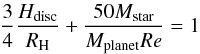 (4)where
Hdisc is the disc scale height at the location of the
planet, and
(4)where
Hdisc is the disc scale height at the location of the
planet, and  is
the Reynolds number at the location of the planet. We use in our model an analytic
description of type I migration, which reproduces the results of Paardekooper et al. (2011), which include the effect of co-rotation
torque and the fact that discs can be non-isothermal. A detailed description of this model
is presented in Dittkrist et al. (in prep.).
is
the Reynolds number at the location of the planet. We use in our model an analytic
description of type I migration, which reproduces the results of Paardekooper et al. (2011), which include the effect of co-rotation
torque and the fact that discs can be non-isothermal. A detailed description of this model
is presented in Dittkrist et al. (in prep.).
3. Planet orbital evolution
A key component of our multiple planetary system model is the calculation of the gravitational interactions between the embryos. This component is not necessary for describing the evolution of a single planet, but for a multiple planetary system, it can be very important. Gravitational interactions can disturb the orbit of planets and, therefore, increase their collision probability, or inversely they can force them to be trapped in resonances, which can reduce the probability of collision. In this section we describe our method to calculate the gravitational interactions between the planets and the collision detection (see Carron2013, for more details).
3.1. Equations of motion
In the N-body part, we treat each planetary embryo as a point mass. A
body is characterized by its position x, its velocity
ẋ, and its mass m. According to
Newton’s law of universal gravitation, the acceleration of the ith body
 can be
written as
can be
written as 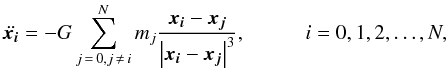 (5)where
G is the gravitational constant and N the number of
planetary bodies. The index 0 refers to the central star.
(5)where
G is the gravitational constant and N the number of
planetary bodies. The index 0 refers to the central star.
Equation 5 can be written for a
heliocentric frame. With the heliocentric position
ri, defined as  (6)and with the
relation
(6)and with the
relation  ,
we can write the equation of motion as
,
we can write the equation of motion as  (7)with
i = 1,2,3...N.
This system of coupled second-order differential equations with 3n
dimensions is solved using a Bulirsch-Stoer integration scheme.
(7)with
i = 1,2,3...N.
This system of coupled second-order differential equations with 3n
dimensions is solved using a Bulirsch-Stoer integration scheme.
3.2. Migration and damping
Migration plays a central role during the formation process of planets. Thanks to the
gravitational interaction between the planets and the gas disc, the planets can move
through the disc. The migration pushes the planets inward or outward depending on the
properties of the disc and the mass of the planet. We use the method of Fogg & Nelson (2007) to include the effect of
disc-planet interaction. The acceleration due to the migration can be written as
 (8)where
tm is the migration timescale defined as
(8)where
tm is the migration timescale defined as
 ,
a is the semimajor axis, and v the velocity of the
body. This timescale is computed following the work of Paardekooper et al. (2011) and depends on the planetary mass, as well as on the
local properties of the disc. Details on the migration timescale computation can be found
in Mordasini et al. (2011) and Dittkrist et al. (in
prep.). This equation is valid for weak migration forces, which means
tm should be much longer than the orbital period.
,
a is the semimajor axis, and v the velocity of the
body. This timescale is computed following the work of Paardekooper et al. (2011) and depends on the planetary mass, as well as on the
local properties of the disc. Details on the migration timescale computation can be found
in Mordasini et al. (2011) and Dittkrist et al. (in
prep.). This equation is valid for weak migration forces, which means
tm should be much longer than the orbital period.
The gravitational interactions of the planets with the gas disc lead to a damping of the eccentricity and of the inclination of the planets. We assume that the eccentricity and inclination damping timescales are similar, and both equal one tenth of the absolute value of the migration timescale. The ratio between the eccentricity (and inclination) and semi-major axis damping timescales is very uncertain, and the value we use there is just a rough order-of-magnitude estimation. We present our tests for inferring the effect of this parameter in Sect. 5.
The accelerations caused by the damping of the eccentricity
ade and of the inclination
adi are calculated as  (9)for
the eccentricity and
(9)for
the eccentricity and  (10)for the
inclination, where k is the unit vector
(0,0,1). Also here, te and
ti should be much longer than the orbital period.
(10)for the
inclination, where k is the unit vector
(0,0,1). Also here, te and
ti should be much longer than the orbital period.
Putting all together we can calculate the total acceleration
at of a planet as
 (11)where
ag is acceleration due to the gravitation of
the other bodies as described in Eq. (7)
with
(11)where
ag is acceleration due to the gravitation of
the other bodies as described in Eq. (7)
with  .
.
3.3. Collision detection
During the evolution of a planetary system, collisions between planets may occur. We detect collisions by checking, after each time step of the N-body code2, that two bodies are closer to each other than the collision distance R, which we define as the sum of both core radii (R = R1 + R2). The numerical integration has an adaptive time step (h), which ensures that an integration with the desired precision is obtained. In addition, we limit the length of the N-body time step to a value less than the collision timescale τ, which is calculated as follows:
-
1.
For each pair of planets k, we approximate the positions r1,r2 of the two bodies at the time t = t0 + Δt:
 where
x1(t0),x2(t0)
are the positions,
v1(t0),v2(t0)
the velocities, and
a1(t0),a2(t0)
the accelerations at the time t0.
where
x1(t0),x2(t0)
are the positions,
v1(t0),v2(t0)
the velocities, and
a1(t0),a2(t0)
the accelerations at the time t0. -
2.
We define τk as the minimum real solution for the collision timescale of the equation:
 (14)With the
substitution
(14)With the
substitution  we
get
we
get  (18)
(18) -
3.
We are only interested in solutions with τk < h, h being the time step of the N-body integrator. If the distance between the two bodies d at the time t0
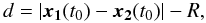 (19)is longer than the
maximum change of the distance Δdmax,
(19)is longer than the
maximum change of the distance Δdmax,
![Mathematical equation: \begin{eqnarray} \begin{array}{lcl} \Delta d_{\max}\! & = &\! \max \left(| \vect{r_1}(t_0 + \tilde \Delta t) - \vect{r_2}(t_0 + \tilde \Delta t)| \; \forall \tilde \Delta t \in [t_0,t_0 + \Delta t] \right) \nonumber \\ \! & = &\! \max \left(| \Delta \vect{v}(t_0 \! + \! \tilde \Delta t) \! +\! \frac{1}{2} \Delta \vect{a}(t_0 \! +\! \tilde \Delta t)^2| \; \forall \tilde \Delta t \in [t_0,t_0 \! +\! \Delta t] \right) \nonumber \end{array} \end{eqnarray}](/articles/aa/full_html/2013/10/aa21690-13/aa21690-13-eq78.png) then,
obviously, no real solution exists with
τk < Δt.
Calculating Δdmax is not trivial; however, we can easily
find a maximum limit of Δdmax using the triangle
inequality:
then,
obviously, no real solution exists with
τk < Δt.
Calculating Δdmax is not trivial; however, we can easily
find a maximum limit of Δdmax using the triangle
inequality: ![Mathematical equation: \begin{eqnarray} \begin{array}{lcl} \Delta d_{\max} \! & = &\! \max \left(| \Delta \vect{v}(t_0 \! +\! \tilde \Delta t) \! +\! \frac{1}{2} \Delta \vect{a}(t_0 \! +\! \tilde \Delta t)^2| \; \forall \tilde \Delta t \in [t_0,t_0 \! +\! \Delta t] \right) \nonumber \\ \! & \le &\! \max \left( \Delta \vect{v}| (t_0 \! +\! \tilde \Delta t) \! +\! | \frac{1}{2} \Delta \vect{a}|(t_0 \! +\! \tilde \Delta t)^2 \; \forall \tilde \Delta t \in [t_0,t_0\! +\! \Delta t] \right) \nonumber \\ \! & = &\! | \Delta \vect{v}| (t_0 + \Delta t) + \frac{1}{2} |\Delta \vect{a}|(t_0 + \Delta t)^2 . \end{array} \end{eqnarray}](/articles/aa/full_html/2013/10/aa21690-13/aa21690-13-eq80.png) This
leads to
This
leads to 
-
4.
We define τ as the minimal τk,wherek = 1...N(N − 1)/2.
Our model is very similar to the one described in Richardson et al. (2000). The only difference is that we use a second-order Taylor series for the approximation of the position instead of a first-order one. Therefore the method is more accurate but has the disadvantage to bring out a fourth-order equation instead of a second-order one.
3.4. Collision handling
After each N-body time step we check for collisions. If one (or more) is found, we merge the colliding bodies: the collisions are treated as fully inelastic. This means that we remove the less massive body and add its mass to the more massive one. We also change the position and velocity of the more massive one so that the total momentum of the centre of mass is conserved.
When two planets merge, the resulting planet has a core mass that is the sum of the two core masses. The envelope mass of the new planet is calculated as follows: we compute the collision energy and compare it to the binding energy of the more massive planet’s envelope. If the former is higher, the envelope of the planet is ejected; otherwise, it is conserved. In the case where both planets are massive, each with large envelopes, our treatment is not accurate. However, we do not expect such collisions to occur, since these planets would probably be captured in mutual resonances and would not collide. For details on the accretion of a solid embryo by a planet with an envelope we refer the reader to Broeg & Benz (2012).
4. Competition for gas and solid accretion
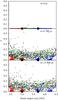 |
Fig. 1 Evolution of the eccentricity (y-axis) and semi-major axis (x-axis, in AU) of a set of test particles under the influence of two planets without gas drag. Particles are coloured according to their initial location: red for particles belonging to the feeding zone of the innermost planet, blue for particles belonging to the feeding zone of the outermost planet, and green for particles belonging to both feeding zones. The two 10 M⊕ planets are located at 5 AU and 5.6 AU. The first panel shows the initial conditions, the second panel is the state after 600 orbital times of the innermost planet, and the last panel is the state after 1200 orbital times of the innermost planet. As can be seen, test particles are very efficiently mixed in the combined feeding zone on a short timescale. Only planetesimals located in co-rotation resonance with one of the two planets are scattered on a longer timescale. |
The planet’s feeding zone is assumed to extend to 4 RHill on both sides of the planet. In case a planet has any eccentricity, the feeding zone extends from amin − 4 RHill to amax + 4 RHill, where amin and amax are the periastron and apoastron. An important effect in our model is the treatment of the feeding zones of planets when they overlap. Indeed, as in Pollack et al. (1996) and A05, for example, our model assumes that the planetesimal surface density in a planet’s feeding zone is uniform. As a consequence, if the two feeding zones of two different planets overlap, the planetesimal surface density in the combined feeding zone itself is constant. This has a number of potentially important consequences:
-
Since a planet’s envelope depends upon its luminosity, which itself depends on the planetesimal accretion rate, hence on the planetesimal surface density, when two feeding zones overlap, the internal structure of the two planets is no longer independent.
-
Two planets sharing their feeding zones compete for the accretion of planetesimals. Interestingly enough, this does not necessarily result in a reduced solid accretion rate. In general, one planet is favoured (its accretion rate is increased compared to the corresponding isolated situation), whereas the other one will grow more slowly. This results simply from the fact that if the two planets compete for the accretion of the same planetesimals (which should result in a decrease in the solid accretion rate for both planets), they also have access to a much larger region of the disc (the union of the two feeding zones of the two planets).
Numerically we proceed as follows. When two feeding zones overlap, we consider that they merge into a big one, its inner limit (ainner) being the minimum of the two inner boundaries of the separated feeding zones, and the outer limit (aout) the maximum of the two outer ones. The surface density of the new feeding zone is considered to be uniform, i.e. the solids surface density of the region is integrated to obtain the total mass, which is then divided by the surface of the feeding zone.
To check that our prescription is a good approximation of reality, we performed N-body calculations, considering two planets and a set of test particles. Figure 1 shows the semi-major axis and eccentricity of the test particles at different times. Particles have different colours depending on their initial location (see caption of Fig. 1). As can be seen in the figure, the planetesimals are indeed very efficiently mixed, resulting in a quasi-uniform surface density (and eccentricity) in a single feeding zone, thus validating our approach.
Planets also compete for the accretion of gas. Indeed, there is a maximum mass a planet can accrete during a given time step. This mass is the sum of the mass already present in the planetary gaseous feeding zone (which is assumed to extend to one Hill’s radius on both sides of the planetary location) and of the mass that can enter in the feeding zone during the time step, as a result of viscous transport (see F13). Since, as already mentioned above, the gas accreted by forming planets is removed from the protoplanetary disc, the mass reservoir and the viscous transport are modified when a planet accretes a large amount of gas (in particular, during the runaway gas accretion). These modifications can in turn modify the maximum mass another planet can accrete.
5. Results
5.1. Formation of a ten-planet system
Before considering a population of planets, we study an example of a ten-planet system formation model. We have considered three models with the same initial conditions. The first one assumes that only one planet forms in the protoplanetary disc3. The second one takes into account the competition between planets for solids and gas accretion, the excitation of planetesimals by all the planets, but not the gravitational interactions between planets. The third model takes into account both the competition for accretion and the gravitational interactions between forming planets: the orbits of planets are computed using the N-body described above. For the three models, the initial surface densities of gas and solids were taken to be 140 g/cm2 and 6 g/cm2 at 5 AU, corresponding to 730 g/cm2 and 8 g/cm2 respectively at 1 AU.
In the second model, we use a very simple prescription for planetary collisions: as soon as two planets have the same semi-major axis, the smallest one is either accreted or ejected by the biggest one. The ratio of ejection to accretion probability is assumed to be the same as for planetesimals (see A05). This is of course a very simplified model, but its only purpose is to emphasize the differences with the third model.
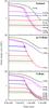 |
Fig. 2 Three models for the formation of 10 planets. Top: formation of 10 independent planets (each of them growing in an identical disc). Middle: the competition for gas and solid accretion, as well as the excitation of planetesimals by all planets, is taken into account. The gravitational interactions between planets are not included. The cross indicates an ejected planet, the big dots indicate collision between planets. Bottom: full model, including the competition for gas and solid accretion, the excitation of planetesimals by all planets, and the gravitational interactions between planets. |
The first model led to a system with ten planets inside 2 AU, and with masses ranging from 0.03 M⊕ to ~12 M⊕ (Fig. 2, upper panel). The results using the second model are presented in Fig. 2, middle panel. The planet that grows more massive is located initially at 5.4 AU, a privileged place in terms of abundance of solids and size of the feeding zone4. During its inward migration it encounters seven other smaller planets, one of which is ejected while the others are accreted. The total mass that the planet gains by accreting other embryos is 0.63 M⊕. In the system, the two outer planets that never suffer from any encounter remain, so in total the system ends up with three planets out of the initial ten. The final masses are 12, 2.9, and 1.5 M⊕, the final locations being 0.16 AU, 1 AU, and 1.8 AU respectively. The formation of the most massive planet is almost identical as if it were growing as an isolated planet. The inner embryos, most of which are accreted, do not favour or slow down the growth of the planet.
As an illustration of the importance of planetary interactions, we note that the final mass of the outermost planet turns out to be 5.6 M⊕, and its final location 0.75 AU (if only one planet is considered), to be compared with 1.5 M⊕ at ~2 AU in the second model. Indeed, in the multi-planet case, accretion is largely reduced when the planet enters regions of the disc already visited by other embryos (and therefore with less material available) and by the fact that random velocities of the (fewer) available planetesimals in these regions are higher due to the perturbations of the other protoplanets. The reduction of solid accretion could also, however, reduce the critical mass, and therefore enhance gas accretion. For this process to happen, however, the reduction of solid accretion must occur for a planet that is already quite massive, a situation that is not encountered in this simulation.
To illustrate the excitation of planetesimals by the ten planets, Fig. 3 shows the eccentricity of planetesimals in the disc as a function of semi major axis and time in the second model. Clearly, at the position of the protoplanets, the eccentricity is the highest. As the planets grow, they perturb the disc to a great extent. In addition, as the disc dissipates, the damping effect of the gas drag decreases, which results in overall higher excitation of planetesimals.
Using the third model, we obtain a different system (see Fig. 2, bottom panel). As we can see, in this case only three planets are accreted by the most massive planet during its inward migration, so the final number of planets in this system is seven. Planets that before were considered to be accreted or ejected survive in the system due to resonance trapping. Also, orbit crossing is possible without the loss or the ejection of the planet. When the gravitational interactions are not considered, small planets that are in the inner part of the disc are usually swept out by a more massive, inwardly migrating planet. However, as we can see from this example, this approximation underestimates the amount of these small, close-in planets. Therefore, accurate formation of planetary systems should account for the gravitational interactions of the protoplanets. To get the proper orbital configurations in planetary systems, N-body calculations are mandatory.
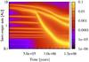 |
Fig. 3 Eccentricity of planetesimals in the disc as a function of time (x-axis) and semi-major axis (y-axis). The colour bar indicates the eccentricity values. In this model, the competition for gas and solid accretion, as well as the excitation of planetesimals by all growing planets, is included. This corresponds to the middle panel of Fig. 2. |
5.2. Planet population
We now present the effect of multi-planetary formation at the population level, by comparing two identical models, one assuming only one planet growing in each protoplanetary disc, the second one assuming that ten planetary embryos grow in each of the discs. We stress that it is not our goal in the present paper to reproduce the observed population of planets, but rather to study the differential effect of having more than one planet forming in a system, using parameters that lead to populations that are not totally at odd with observations.
5.2.1. Initial conditions
The initial conditions are given by the characteristics of a protoplanetary disc, and the ensemble of planetary embryos, whose initial mass and semi-major axis are computed in the following way. The starting location of the planetary embryos is selected at random, using a probability distribution uniform in log. It ranges from 0.1 AU to 20 AU. We moreover impose that two planetary embryos should not start closer than 10 times their mutual Hill radius. The initial mass of the planetary embryos is assumed to be equal to 10-2 M⊕.
The initial gas disc surface density profiles we consider are given by
![Mathematical equation: \begin{equation} \Sigma = (2 - \gamma) { \mdisk \over 2 \pi \ac ^{2-\gamma} \rzero^\gamma } \left( {r \over \rzero} \right)^{-\gamma} \exp \left[ - \left( {r \over \ac} \right) ^{2-\gamma} \right] , \end{equation}](/articles/aa/full_html/2013/10/aa21690-13/aa21690-13-eq98.png) (20)where
r0 is equal to 5.2 AU, and
Mdisc, aC, γ
are derived from the observations of Andrews et al.
(2010). For numerical reasons, the innermost disc radius,
rinner is taken at 0.05 AU, and differs in some cases from
the one cited in Andrews et al. (2010). Although
Andrews et al. (2010) derive a value for the
viscosity parameter α, we assume for simplicity that the viscosity
parameter is the same for all the protoplanetary discs considered. Using a different
α parameter will be the subject of future work. We assume that the
mass of the central star is 1 M⊙.
(20)where
r0 is equal to 5.2 AU, and
Mdisc, aC, γ
are derived from the observations of Andrews et al.
(2010). For numerical reasons, the innermost disc radius,
rinner is taken at 0.05 AU, and differs in some cases from
the one cited in Andrews et al. (2010). Although
Andrews et al. (2010) derive a value for the
viscosity parameter α, we assume for simplicity that the viscosity
parameter is the same for all the protoplanetary discs considered. Using a different
α parameter will be the subject of future work. We assume that the
mass of the central star is 1 M⊙.
Characteristics of disc models.
As in Mordasini et al. (2009a,b, M09a; M09b, the planetesimal-to-gas ratio is assumed to scale with the metallicity of the central star, with a ratio of 0.04 for solar metallicity. For the disc models we consider, this corresponds to solid surface densities ranging from 0 to 10 g/cm2 at 5.2 AU, with a long-tail distribution extending up to 50 g/cm2. For every protoplanetary disc we consider, we therefore select at random the metallicity of a star from a list of ~1000 CORALIE targets (Santos, priv. comm.). Finally, following Mamajek (2009), we assume that the cumulative distribution of disc lifetimes decays exponetially with a characteristic time of 2.5 Myr. When a lifetime Tdisc is selected, we adjust the photoevaporation rate so that the protoplanetary disc mass reaches 10-5M⊙ at the time t = Tdisc, when we stop the calculation.
5.2.2. Mass versus semi-major axis diagrams
The number of planetary embryos we consider in each protoplanetary disc is a free parameter. In order to ease the comparison between the two computations, the total number of planets in each case is similar (at least at the beginning of the calculation): we have considered 500 systems with ten planets, and ~5000 systems with only one planet. The initial locations of planets, in the two cases, are statistically the same, but, as opposed to what was presented in Sect. 5.1, the starting location of planets in the one-planet case are not exactly the same as in the ten-planet case.
Figure 4 shows the mass versus semi-major axis diagram of synthetic planets, in the case where only one planet forms in the system (case 1). The colour code is related to the composition of the planetary core, which itself is the result of the accretion of different kinds of planetesimals (icy planetesimals or rocky planetesimals). Figure 5 presents the same results, but in the case of ten planets per system.
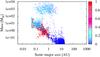 |
Fig. 4 Mass versus semi-major axis diagram for a population of planets, assuming one planet grows in each disc. The colour code shows the fraction of rocky planetesimals accreted by the planet. Planets whose core is the result of the accretion of rocky planetesimals are in red, whereas planets whose core has been made by the accretion of icy planetesimals are in blue. The total number of point is 4936. Planets in the vertical line at 0.05 AU are planets that reached the inner boundary of the computed disc. If the computational domain were extended to lower semi-major axis, their fate is uncertain. They could continue migrating toward the central star and be accreted, or could stop their migration somewhere in the inner disc cavity. |
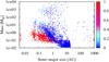 |
Fig. 5 Same as Fig. 4, but assuming now that ten planetary embryos are growing and migrating in every protoplanetary disc. The number of points is 5010. Planets on the vertical line at 1000 AU are planets ejected from the system. Their mass represents their mass at the time of ejection. Planets on the vertical line at 0.005 AU are planets that have collided with the central star. We do not include in our models planet-star interactions that could modify the orbital evolution of planets in the innermost parts of the disc. |
After comparing the two diagrams (Figs. 4 and 5), it appears clearly that not all planets (in terms of mass and semi-major axis) are affected in the same way by the presence of other bodies. In particular, the sub-population of massive planets does not seem to be affected as much, although planets in the ten-planet case are slightly less massive. Another interesting difference is that planets in the one-planet case are located closer to the central star, still in the same mass domain. The origin of both differences is the competition between planets forming in the same disc. As planets compete for the accretion of solids, their growth is delayed. They start to migrate later in the disc lifetime and start to accrete gas in a runaway mode at a later time. As a consequence, their final location is somewhat further out than in the one-planet case, and their mass is lower. (The mass of the planets is plotted using a logarithmic scale, which decreases the visual difference between the two populations.)
In the sub-population of low-mass planets, in particular close to the central star, the effect of multiplicity is very important. In the ten-planet case, a population of close-in Earth- to super-Earth mass planets appears, whereas this region is empty in the case of one-planet systems. This difference stems from the gravitational interactions between planets in the same system. At a fraction of an AU from the central star, the mass of solids (these planets are made almost totally from solids) is not high enough to grow a planet of a few Earth masses, at least not for the disc masses we consider here. On the other hand, disc-planet angular-momentum exchange alone (leading to migration) is not strong enough for these planets to move planets from the outside toward this region. As a consequence, planets at these distance are either less massive than the Earth or more massive than ~10 M⊕. In the case of a multi-planetary system, planets interact gravitationally with another member of the same system, which itself is massive enough to migrate appreciably. As a consequence, an inner, low-mass planet can be pushed by resonant interaction toward the inner parts of the protoplanetary disc. However, this does not imply that the different planets are in mean-motion resonance at the end of the protoplanetary disc lifetime. Indeed, depending on the planetary mass, a mean-motion resonance can be broken during a later phase of disc evolution.
A third sub-population that is notably different between the two cases is the population of planets below 0.05 AU, at all masses. The difference again stems from the resonant interaction between planets. In the one-planet case, since the protoplanetary disc is assumed to only extend down to 0.05 AU, migration ceases for planets below this radius. In the ten-planet case, on the other hand, planets can suffer resonant interaction and enter the innermost parts of the disc. It should be noted, however, that this difference depends strongly on the adopted value of the disc inner cavity radius.
A fourth difference is related to planets located at large distances from their central star. Obviously, since the initial location of the planets is assumed to be smaller than 20 AU, planets in the one-planet case are all located in the inner regions of the disc. (Although planets can migrate outwards during some phases of their formation, they generally terminate their migration at a position closer to the star than the initial one.) In the ten-planet case, gravitational interactions between planets can lead to the scattering of planets either towards the outer regions of the disc (few hundreds of AU), or to ejecting them from the system alltogether (the outer boundary of the system is assumed to be at 1000 AU). Some of the planets ejected from the inner regions of the system, but still bound to the star, are quite massive and could be compared with planets detected by direct imaging (e.g. Marois et al. 2008; Kalas et al. 2008; Lagrange et al. 2009).
Interestingly enough, there seems to be a lack of massive planets at “intermediate” distances (50–100 AU). It is not presently clear if this is an effect of not having enough statistics, or if this is a real effect (for example due to the initial location of planetary embryos, assumed to be below 20 AU). In addition, microlensing surveys have recently claimed to have discovered a large population of massive free-floating planets. As can be seen in Fig. 5, planets with very high masses can indeed be ejected from the system during formation. We finally note that the results presented in Fig. 5 correspond to the state of the system at the time the gas disc vanishes. We do not include the long-term evolution of planetary systems in these calculations. Such a study, and the study of the resulting eccentricity evolution of planets, is beyond the scope of this paper but will be considered in a forthcoming work (Pfyffer et al., in prep.). Such effects could increase the number of ejected planets and, as a consequence, the number of expected free-floating planets.
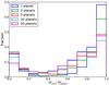 |
Fig. 6 Distribution of the fraction of heavy elements Mcore/Mplanet for the same simulations, differing only by the assumed number of planetary embryos per system. Only planets more massive than 1M⊕ have been considered in these distributions. |
Finally, a last difference is in the composition of planets, in particular in the super-Earth mass domain. Indeed, planets in this mass range are notably richer in volatile elements in the ten-planet case than in the one-planet case. The origin of this difference is again related to a modified migration of planets, thanks to gravitational interactions. The ice line is located in our disc at a few AUs from the central star. As a consequence, planets below 1 AU are in general devoid of volatiles, except if they are massive enough to have migrated significantly. On the other hand, in the multi-planet case, low-mass planets, which start their formation in the cold parts of the disc (where planetesimals are volatile rich), can be pushed to the volatile poor regions of the disc by another external and more massive planet. While this effect is likely to be quantitatively modified including the orbital drifting of planetesimals as a result of gas drag, this effect should qualitatively remain present in more detailed models.
Also related to the composition of planets, we have compared the mean metallicity of planets in the different cases. For this, we have plotted in Fig. 6 the histogram of Mcore/Mplanet for the different cases we considered (including the calculations with 2, 5, and 20 planetary embryos, see below). Interestingly enough, the mean heavy element fraction increases for planets forming in systems. This effect can be explained as follows: planets forming in systems acquire their mass on a longer timescale (compared to single planets). As a consequence, they reach the critical mass later, and have less time (until the gas disc dissipates) to accrete gas.
In both populations, models predict there is a population of low-mass objects at distances between a few AU and 20 AU. These represent planetary embryos that have not managed to grow larger than a fraction of an Earth mass. Their outermost location (20 AU) is simply the effect of the assumed initial location of planetary embryos (which only extends to 20 AU). Their innermost location corresponds to places in the disc where the solid accretion rate of solids is so small that planetary embryos do not grow noticeably during the lifetime of the gas disc.
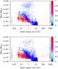 |
Fig. 7 Same model as in Fig. 5, except that 5 (top) or 20 (bottom) embryos are assumed to form in the same protoplanetary disc. The number of points are 4875 and 5000, respectively. |
6. Discussion and conclusions
6.1. Effect of multiplicity
In the previous section, we have presented the differential effects of considering the formation of more than one planet in the same disc. However, there are parameters that could potentially have important effects on the results. In particular, we considered the growth and migration of ten planetary embryos, and one may wonder what would result if this number was changed. In addition, we mentioned earlier that the timescale for damping of the planet’s eccentricity and inclination is theoretically poorly known.
To check on the sensitivity of our results to the number of starting embryos used, we initiated a set of additional simulations with 2, 5, and 20 embryos. The resulting masses and semi-major axis diagrams for the simulations with 5 and 20 planets are depicted in Fig. 7. As can be seen in the two figures, and after comparing with Fig. 5, the effect of the number of embryos is modest, at least on the mass versus semi-major axis diagram, because globally the overall structure is similar. One can note, however, that the population of planets at large distances (beyond 50 AU) is larger in the case of 20 planetary embryos. Moreover, the population of massive planets (larger than Jupiter) is smaller in the 20-planet case. Finally, a population of intermediate planets (from super-Earth to Neptune mass) at a few AU appears in the 20-planet case.
 |
Fig. 8 Top: mean number of planets per system that are more massive than a given value, for different simulations, assuming different numbers of planetary embryos initially present in the system. Middle: cumulative mass function, considering only planets more massive than 5 M⊕ still present in the system at the end of the simulation (planets colliding with the central star or ejected are not considered). Bottom: cumulative distribution of semi-major axis for the same population as in the middle panel. The number of planetary embryos assumed in each set of simulation is indicated on the panels. In the bottom panel, the planets that have been transported inside 0.05 AU by gravitational interactions with other planets of the same system. |
To quantify the effect of the initial number of planetary embryos, we have also computed the average number (per system) of planets larger than a given value, and compared the results for the same set of simulations (assuming 1, 2, 5, 10, or 20 planetary embryos are initially present in the same disc). As before, the initial locations of planetary embryos are statistically similar in all the cases. As can be seen in Fig. 8 (top panel), all the curves converge for high-mass planets, but diverge towards the lower mass end. Simulations assuming a larger number of planetary embryos tend to lead to the formation of more low-mass planets, which is somewhat expected. Another interesting aspect is that one notes a convergence of the curves as the number of planetary embryos increases. We can conclude, for example, that simulations assuming 10 or 20 planetary embryos lead to similar results if one only considers planets more massive than a few M⊕.
Considering the cumulative distribution of planetary masses (Fig. 8, middle panel), taking objects more massive than 5 M⊕ into account, it is clear that the mass function converges for more than ten planetary embryos (see the light blue and purple lines). The distribution of semi-major axis also presents a convergence for more than ten planetary embryos (Fig. 8, bottom panel). Only planets that are present in the system at the end of the simulation are considered in this plot. Planets ejected or accreted by the central star are not considered in the calculation. If one now considers all the planets, the fraction of ejected planets increases monotonically with the number of planetary embryos initially present in the simulation, from nearly 0 for 2 planetary embryos, to 3%, 5%, and 8% for 5, 10, and 20 planetary embryos respectively.
It is also interesting to compare the period ratios we obtain, as a function of the number of planetary embryos initially present in the system. Figure 9 presents the period ratios of all planets more massive than 5 M⊕, for the different simulations presented above (starting with 5, 10, or 20 planetary embryos). As can be seen in the figure, the importance of the mean-motion resonances decreases when the number of planetary embryos increases (see also Rein 2012): in the case of two planetary embryos, nearly all the systems end in mean-motion resonance, whereas this fraction is much smaller in the case of 20 planetary embryos. Unlike the mass and semi-major cumulative histograms, there is still a difference between the cases with 10 and 20 planetary embryos, which means that the precise architecture of planetary systems depends on the amount of planetary embryos assumed to be present in the system.
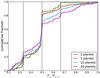 |
Fig. 9 Period ratio of all pairs of planets more massive than 5 M⊕, for different simulations assuming initially different numbers of planetary embryos. The vertical lines show the location of the most important mean-motion resonances. |
6.2. Eccentricity and inclination damping
We also tested the effect of the timescale of planet’s eccentricity and inclination damping, assuming a damping timescale increased by a factor 10, or no damping at all (Fig. 11). This simulation obviously resulted in an increased mean eccentricity of planets, at the end of the formation process (see Fig. 10). However, the masses and semi-major axes of planets that survived the formation were not too different from the standard ten-planet case presented in Fig. 5. The main difference can be seen in the population of planets at distances between 10 and 100 AUs and the number of ejected planets, which are more numerous in the low damping case. Interestingly enough, the comparison between the number of planets at these distances, with the results of future direct imaging surveys, could put some constraints on these components of the model.
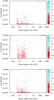 |
Fig. 10 Semi-major axis versus eccentricity for three models. Top: nominal ten-planet model. Middle: without eccentricity and inclination damping. Bottom: with eccentricity and inclination damping timescales increased by a factor 10 compared to the nominal model. The colour code indicates the mass of the planet, in Earth masses (on log scale). |
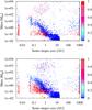 |
Fig. 11 Same model as in Fig. 5, with modified eccentricity and inclination damping for planets. Top: no damping, bottom: damping timescale increased by 10 compared to the nominal case. The number of points are 4650 and 5030, respectively. |
Interestingly enough, the period ratios obtained with less damping, or else without any damping of eccentricity and inclination, seem to be closer to the ones observed by Kepler (in particular, the fraction of planets close to mean-motion resonance is decreased when the damping is reduced). Indeed, in our nominal ten-planet case, a larger fraction of planets than observed find themselves at mean-motion resonances at the end of their formation. This suggests that the eccentricity and inclination damping is overestimated in our models. A more detailed analysis of this effect, as well as comparisons with Kepler results, will be presented in a forthcoming paper.
6.3. Limitations of the model
As for all theoretical models, the one presented in this paper is limited in certain aspects. To put our results in perspective, we now list some of the most important assumptions and limitations. This will also provide a list of work we intend to do in the future.
6.3.1. Planetesimal disc
The numerical treatment of the disc of planetesimals is, in this work, simple, because the characteristics of planetesimals only depend on their semi-major axis. This is the case for the mass (or radius), as well as for the eccentricity and inclination. More specifically, we compute the evolution of the r.m.s eccentricity and inclination of planetesimals, assuming that they are well described by a Rayleigh distribution.
Although it constitutes an improvement with regard to former models (e.g. A05; M09a; M09b; M12b), where the excitation and damping of planetesimals by forming planets and gas drag was not computed accurately, this approach is limited in the sense that some important processes are not included. Among them, one can cite the orbital drifting of planetesimals, due to gas drag, as well as the formation of a gap in the planetesimal disc.
Moreover, as already mentioned, the mass of planetesimals at a given radius does not evolve with time, implying that fragmentation and mass growth of planetesimals are not included. We plan to improve these aspects by using a model similar to the one recently proposed by Ormel & Kobayashi (2012). Finally, planetesimals have no effect on the orbital evolution of planets in this model: the planetesimal driven migration (e.g. Ormel et al. 2012) and the damping of eccentricity and inclination by planetesimals are not included in the model. These effects could indeed be potentially very important in regions of the disc where the gas surface density is low (e.g. outer parts of the disc) or at the end of the disc lifetime, and during long-term evolution.
6.3.2. Planet-planet interaction through the protoplanetary disc
As mentioned at the beginning of this paper, some interactions between planets are mediated by the gas phase of the protoplanetary disc. Indeed, if massive enough, a first planet is likely to modify the gas surface density in a substantial way, therefore modifying angular-momentum exchange and migration. Such effects have been studied in different papers (e.g. Masset & Snellgrove 2001; Morbidelli & Crida 2007). In particular, it is suspected that, when two planets grow massive enough to open a gap in the disc, and when these two gaps merge, the angular momentum evolution of the whole system can lead, under certain conditions (e.g. related to the mass ratio between the two planets), to outward migration of both planets, catching them in mean-motion resonance. This process is in particular believed to have been at work during the late stage of the formation of the solar system (e.g. Walsh et al. 2011). We plan to specifically investigate the formation of the solar system in a forthcoming paper.
6.3.3. Long term evolution
As already mentioned above, we focus in this formation model on the mass growth and orbital evolution of planets in planetary systems during the existence of the gas phase of the protoplanetary disc. The reason for this limitation is that we mainly consider the formation of planets with non-negligible gas envelopes, whose growth is stopped when the gas disc has disappeared. Moreover, a large fraction of planetesimals have either been ejected or accreted by planets at the end of the protoplanetary (gas) disc life, when we stop the computation. We therefore expect that planets should not notably grow after this period, except as a result of collisions between planets or planetary embryos.
The disappearance of the protoplanetary disc however has not only the consequence of stopping the mass growth (in terms of gas) of planets, but it also means the end of eccentricity and inclination damping of planets. As a result, the dynamical state of planetary systems is likely to evolve, leading to a re-arrangement of the architecture of systems. We performed test calculations of the evolution of the planetary systems presented in this paper, and have found that the mass and semi-major axis of planets are not strongly modified, at least at the population level. The long-term interaction between planets, however, has an effect in the increase in planetary eccentricities. Such calculations will be presented in a forthcoming paper (Pfyffer et al., in prep.).
6.3.4. Planetary internal structure
The models presented here are derived closely from the former models presented in A05, M12a, M12b, and F13. In particular, it is assumed, when we compute the internal structure of forming planets, that all accreted planetesimals reach the planetary core, depositing at this location their mass and energy. It is however likely that planetesimals, in particular those of low mass, are destroyed during their travel towards the planetary centre. This leads to a modification of the core luminosity, a reduced core growth, and an increase of the metallicity of the planetary envelope.
It has been recently shown (Hori & Ikoma 2011) that a change in the mean opacity and equation of state in the planetary envelope, itself resulting from the destruction of incoming planetesimals, can heavily modify the planetary critical mass, and therefore the whole planet formation timescale. The aforementioned study assumed some value of the metallicity in the planetary envelope, which is not computed as a result of planet formation. It is, however, more likely that the metallicity of planets will change with time, as a result of the accretion of planetesimals and as a function of the stability of the envelope with regards to convection. Indeed, if convection is efficient enough, the heavy elements deposited by planetesimals are likely to be equally distributed in the whole convective zone, whereas heavy elements and grains could settle down in the radiative zone. Such a self-consistent computation of the planetary internal structure and its effect on the planetary growth and migration will be studied in a forthcoming paper.
6.4. Conclusion
We have extended our planet formation model to include the formation of planetary systems. For this, we seeded our simulations with a number (ranging from 2 to 20) of small seed embryos. We showed that the presence of several growing embryos can result in very important modifications in the overall formation process. In particular, gravitational interactions between these growing bodies results in significant changes in the final mass, semi-major axis and orbital parameters, in particular as a result of the larger orbital migration of planets, which itself results from planet-planet interactions. As a result, planets belonging to planetary systems are found to be richer in water in the region around 1 AU, and a population of low-mass, close-in planets appears, which is not present when considering the growth of only one planet.
We also demonstrated that the mass distribution and cumulative distribution of planets do not strongly depend on the number of planetary embryos considered, in particular for planets more massive than a few Earth masses. However, the distribution of period ratios between planets does depend on the number of planetary embryos, even if the dependance seems to decrease with the number of embryos. The distribution of period ratios also shows that our model predicts too many systems in, or close to, mean-motion resonance. This could result from effects that are not taken into account in our model, for example, from stochastic effects (see e.g. Rein 2012), or from an overestimation of the eccentricity and inclination damping in our model. Future work will address these issues, as well as the ones presented in the previous sections.
Here, we do not include the radial drift of planetesimals. Therefore, planetesimals actually enter the feeding zone of another planet, if the feeding zone borders themselves move as a result of planetary growth and migration. The computation of the orbital drift of planetesimals will be the subject of future work.
The time step for the N-body is in general much shorter than the time step required to compute planetary growth.
This means that we ran ten independent models, varying only the initial location of the planetary embryo, which are taken as the same initial location of planets in the ten-planet case.
The ice line is located at 2.8 AU, and the planet starting at 5.4 AU is the planet starting both outside the ice-line, and closer to the star than the others.
Acknowledgments
This work was supported by the European Research Council under grant 239605, the Swiss National Science Foundation, and the Alexander von Humboldt Foundation.
References
- Alibert, Y., Mordasini, C., Benz, W., & Winisdoerffer, C. 2005a, A&A, 434, 343 [NASA ADS] [CrossRef] [EDP Sciences] [Google Scholar]
- Alibert, Y., Mousis, O., Mordasini, C., & Benz, W. 2005b, ApJ, 626, L57 [NASA ADS] [CrossRef] [Google Scholar]
- Alibert, Y., Baraffe, I., Benz, W., et al. 2006, A&A, 455, L25 [NASA ADS] [CrossRef] [EDP Sciences] [Google Scholar]
- Andrews, S. M., Wilner, D. J., Hughes, A. M., Qi, C., & Dullemond, C. P. 2010, ApJ, 723, 1241 [NASA ADS] [CrossRef] [Google Scholar]
- Borucki, W. J., Koch, D. G., Basri, G., et al. 2011, ApJ, 728, 117 [NASA ADS] [CrossRef] [Google Scholar]
- Broeg, C. H., & Benz, W. 2012, A&A, 538, A90 [NASA ADS] [CrossRef] [EDP Sciences] [Google Scholar]
- Carron, F. 2013, Ph.D. Thesis, University of Bern [Google Scholar]
- Crida, A., Morbidelli, A., & Masset, F. 2006, Icarus, 181, 587 [Google Scholar]
- Fogg, M. J., & Nelson, R. P. 2007, A&A, 472, 1003 [NASA ADS] [CrossRef] [EDP Sciences] [MathSciNet] [Google Scholar]
- Fortier, A., Alibert, Y., Carron, F., Benz, W., & Dittkrist, K.-M. 2013, A&A, 549, A44 [NASA ADS] [CrossRef] [EDP Sciences] [Google Scholar]
- Guilera, O. M., Brunini, A., & Benvenuto, O. G. 2010, A&A, 521, A50 [NASA ADS] [CrossRef] [EDP Sciences] [Google Scholar]
- Guilera, O. M., Fortier, A., Brunini, A., & Benvenuto, O. G. 2011, A&A, 532, A142 [NASA ADS] [CrossRef] [EDP Sciences] [Google Scholar]
- Hori, Y., & Ikoma, M. 2011, MNRAS, 416, 1419 [NASA ADS] [CrossRef] [Google Scholar]
- Inaba, S., & Ikoma, M. 2003, A&A, 410, 711 [NASA ADS] [CrossRef] [EDP Sciences] [Google Scholar]
- Johansen, A., Oishi, J. S., Mac Low, M.-M., et al. 2007, Nature, 448, 1022 [Google Scholar]
- Kalas, P., Graham, J. R., Chiang, E., et al. 2008, Science, 322, 1345 [NASA ADS] [CrossRef] [PubMed] [Google Scholar]
- Lagrange, A.-M., Gratadour, D., Chauvin, G., et al. 2009, A&A, 493, L21 [NASA ADS] [CrossRef] [EDP Sciences] [Google Scholar]
- Lissauer, J. J., Fabrycky, D. C., Ford, E. B., et al. 2011, Nature, 470, 53 [NASA ADS] [CrossRef] [PubMed] [Google Scholar]
- Lovis, C., Ségransan, D., Mayor, M., et al. 2011, A&A, 528, A112 [NASA ADS] [CrossRef] [EDP Sciences] [Google Scholar]
- Mamajek, E. E. 2009, in AIP Conf. Ser. 1158, eds. T. Usuda, M. Tamura, & M. Ishii, 3 [Google Scholar]
- Marois, C., Macintosh, B., Barman, T., et al. 2008, Science, 322, 1348 [NASA ADS] [CrossRef] [PubMed] [Google Scholar]
- Masset, F., & Snellgrove, M. 2001, MNRAS, 320, L55 [NASA ADS] [CrossRef] [Google Scholar]
- Masset, F. S., Morbidelli, A., Crida, A., & Ferreira, J. 2006, ApJ, 642, 478 [NASA ADS] [CrossRef] [Google Scholar]
- Mayor, M., & Queloz, D. 1995, Nature, 378, 355 [NASA ADS] [CrossRef] [Google Scholar]
- Mayor, M., Marmier, M., Lovis, C., et al. 2011, A&A, submitted [arXiv:astro-ph/1109.2497] [Google Scholar]
- Min, M., Dullemond, C. P., Kama, M., & Dominik, C. 2011, Icarus, 212, 416 [NASA ADS] [CrossRef] [Google Scholar]
- Morbidelli, A., & Crida, A. 2007, Icarus, 191, 158 [NASA ADS] [CrossRef] [Google Scholar]
- Mordasini, C., Alibert, Y., & Benz, W. 2009a, A&A, 501, 1139 [NASA ADS] [CrossRef] [EDP Sciences] [Google Scholar]
- Mordasini, C., Alibert, Y., Benz, W., & Naef, D. 2009b, A&A, 501, 1161 [NASA ADS] [CrossRef] [EDP Sciences] [Google Scholar]
- Mordasini, C., Dittkrist, K.-M., Alibert, Y., et al. 2011, in IAU Symp. 276, eds. A. Sozzetti, M. G. Lattanzi, & A. P. Boss, 72 [Google Scholar]
- Mordasini, C., Alibert, Y., Georgy, C., et al. 2012a, A&A, 547, A112 [NASA ADS] [CrossRef] [EDP Sciences] [Google Scholar]
- Mordasini, C., Alibert, Y., Klahr, H., & Henning, T. 2012b, A&A, 547, A111 [NASA ADS] [CrossRef] [EDP Sciences] [Google Scholar]
- Movshovitz, N., Bodenheimer, P., Podolak, M., & Lissauer, J. J. 2010, Icarus, 209, 616 [NASA ADS] [CrossRef] [Google Scholar]
- Ormel, C. W., & Kobayashi, H. 2012, ApJ, 747, 115 [NASA ADS] [CrossRef] [Google Scholar]
- Ormel, C. W., Ida, S., & Tanaka, H. 2012, ApJ, 758, 80 [NASA ADS] [CrossRef] [Google Scholar]
- Paardekooper, S.-J., Baruteau, C., Crida, A., & Kley, W. 2010, MNRAS, 401, 1950 [NASA ADS] [CrossRef] [Google Scholar]
- Paardekooper, S.-J., Baruteau, C., & Kley, W. 2011, MNRAS, 410, 293 [NASA ADS] [CrossRef] [Google Scholar]
- Pollack, J. B., Hubickyj, O., Bodenheimer, P., et al. 1996, Icarus, 124, 62 [NASA ADS] [CrossRef] [Google Scholar]
- Rein, H. 2012, MNRAS, 427, L21 [NASA ADS] [Google Scholar]
- Richardson, D. C., Quinn, T., Stadel, J., & Lake, G. 2000, Icarus, 143, 45 [NASA ADS] [CrossRef] [Google Scholar]
- Shakura, N. I., & Sunyaev, R. A. 1973, A&A, 24, 337 [NASA ADS] [Google Scholar]
- Tanaka, H., Takeuchi, T., & Ward, W. R. 2002, ApJ, 565, 1257 [NASA ADS] [CrossRef] [Google Scholar]
- Veras, D., & Armitage, P. J. 2004, MNRAS, 347, 613 [NASA ADS] [CrossRef] [Google Scholar]
- Walsh, K. J., Morbidelli, A., Raymond, S. N., O’Brien, D. P., & Mandell, A. M. 2011, Nature, 475, 206 [NASA ADS] [CrossRef] [PubMed] [Google Scholar]
- Ward, W. R. 1997, ApJ, 482, L211 [NASA ADS] [CrossRef] [Google Scholar]
All Tables
All Figures
|
Fig. 1 Evolution of the eccentricity (y-axis) and semi-major axis (x-axis, in AU) of a set of test particles under the influence of two planets without gas drag. Particles are coloured according to their initial location: red for particles belonging to the feeding zone of the innermost planet, blue for particles belonging to the feeding zone of the outermost planet, and green for particles belonging to both feeding zones. The two 10 M⊕ planets are located at 5 AU and 5.6 AU. The first panel shows the initial conditions, the second panel is the state after 600 orbital times of the innermost planet, and the last panel is the state after 1200 orbital times of the innermost planet. As can be seen, test particles are very efficiently mixed in the combined feeding zone on a short timescale. Only planetesimals located in co-rotation resonance with one of the two planets are scattered on a longer timescale. |
| In the text | |
|
Fig. 2 Three models for the formation of 10 planets. Top: formation of 10 independent planets (each of them growing in an identical disc). Middle: the competition for gas and solid accretion, as well as the excitation of planetesimals by all planets, is taken into account. The gravitational interactions between planets are not included. The cross indicates an ejected planet, the big dots indicate collision between planets. Bottom: full model, including the competition for gas and solid accretion, the excitation of planetesimals by all planets, and the gravitational interactions between planets. |
| In the text | |
|
Fig. 3 Eccentricity of planetesimals in the disc as a function of time (x-axis) and semi-major axis (y-axis). The colour bar indicates the eccentricity values. In this model, the competition for gas and solid accretion, as well as the excitation of planetesimals by all growing planets, is included. This corresponds to the middle panel of Fig. 2. |
| In the text | |
|
Fig. 4 Mass versus semi-major axis diagram for a population of planets, assuming one planet grows in each disc. The colour code shows the fraction of rocky planetesimals accreted by the planet. Planets whose core is the result of the accretion of rocky planetesimals are in red, whereas planets whose core has been made by the accretion of icy planetesimals are in blue. The total number of point is 4936. Planets in the vertical line at 0.05 AU are planets that reached the inner boundary of the computed disc. If the computational domain were extended to lower semi-major axis, their fate is uncertain. They could continue migrating toward the central star and be accreted, or could stop their migration somewhere in the inner disc cavity. |
| In the text | |
|
Fig. 5 Same as Fig. 4, but assuming now that ten planetary embryos are growing and migrating in every protoplanetary disc. The number of points is 5010. Planets on the vertical line at 1000 AU are planets ejected from the system. Their mass represents their mass at the time of ejection. Planets on the vertical line at 0.005 AU are planets that have collided with the central star. We do not include in our models planet-star interactions that could modify the orbital evolution of planets in the innermost parts of the disc. |
| In the text | |
|
Fig. 6 Distribution of the fraction of heavy elements Mcore/Mplanet for the same simulations, differing only by the assumed number of planetary embryos per system. Only planets more massive than 1M⊕ have been considered in these distributions. |
| In the text | |
|
Fig. 7 Same model as in Fig. 5, except that 5 (top) or 20 (bottom) embryos are assumed to form in the same protoplanetary disc. The number of points are 4875 and 5000, respectively. |
| In the text | |
|
Fig. 8 Top: mean number of planets per system that are more massive than a given value, for different simulations, assuming different numbers of planetary embryos initially present in the system. Middle: cumulative mass function, considering only planets more massive than 5 M⊕ still present in the system at the end of the simulation (planets colliding with the central star or ejected are not considered). Bottom: cumulative distribution of semi-major axis for the same population as in the middle panel. The number of planetary embryos assumed in each set of simulation is indicated on the panels. In the bottom panel, the planets that have been transported inside 0.05 AU by gravitational interactions with other planets of the same system. |
| In the text | |
|
Fig. 9 Period ratio of all pairs of planets more massive than 5 M⊕, for different simulations assuming initially different numbers of planetary embryos. The vertical lines show the location of the most important mean-motion resonances. |
| In the text | |
|
Fig. 10 Semi-major axis versus eccentricity for three models. Top: nominal ten-planet model. Middle: without eccentricity and inclination damping. Bottom: with eccentricity and inclination damping timescales increased by a factor 10 compared to the nominal model. The colour code indicates the mass of the planet, in Earth masses (on log scale). |
| In the text | |
|
Fig. 11 Same model as in Fig. 5, with modified eccentricity and inclination damping for planets. Top: no damping, bottom: damping timescale increased by 10 compared to the nominal case. The number of points are 4650 and 5030, respectively. |
| In the text | |
Current usage metrics show cumulative count of Article Views (full-text article views including HTML views, PDF and ePub downloads, according to the available data) and Abstracts Views on Vision4Press platform.
Data correspond to usage on the plateform after 2015. The current usage metrics is available 48-96 hours after online publication and is updated daily on week days.
Initial download of the metrics may take a while.