| Issue |
A&A
Volume 558, October 2013
|
|
|---|---|---|
| Article Number | A52 | |
| Number of page(s) | 7 | |
| Section | Extragalactic astronomy | |
| DOI | https://doi.org/10.1051/0004-6361/201321402 | |
| Published online | 03 October 2013 | |
Is the Sunyaev-Zeldovich effect responsible for the observed steepening in the spectrum of the Coma radio halo?
1
INAF – Istituto di Radioastronomia, via P. Gobetti 101,
40129
Bologna,
Italy
e-mail: brunetti@ira.inaf.it
2
Minnesota Inst. for Astrophysics, School of Physics &
Astronomy, Univ. of Minnesota, 116
Church Street SE, Minneapolis, MN
55455,
USA
3
Dipartimento di Fisica, Universita’ degli Studi di Roma “Tor
Vergata”, via della Ricerca
Scientifica 1, 00133
Roma,
Italy
4
Universitätssternwarte München, Scheinerstr. 1, 81679
München,
Germany
Received:
4
March
2013
Accepted:
19
August
2013
Aims. The radio halo in the Coma cluster is unique in that its spectrum has been measured over almost two decades in frequency. The current radio data show a steepening of the spectrum at higher frequencies, which has implications for models of the radio halo origin. There is an on-going debate on the possibility that the observed steepening of the spectrum and the apparent shrinking of the halo-size at higher frequencies is not intrinsic to the emitted radiation, but is instead caused by the Sunyaev-Zeldovich (SZ) effect.
Methods. Recently, the Planck satellite obtained unprecedented measurements of the SZ signal and its spatial distribution in the Coma cluster, allowing a conclusive testing of this hypothesis. Using the Planck results, we calculated the modification of the radio halo spectrum by the SZ effect in three different ways. With the first two methods we measured the SZ-decrement by adopting self-consistently the aperture radii used for flux measurements of the radio halo at the different frequencies. First we adopted the global compilation of data-points from Thierbach et al. (2003, A&A, 397, 53) and a reference aperture radius consistent with those used by various authors. Second we used the available brightness profiles of the halo at different frequencies to derive the spectrum of the halo within two fixed apertures, corresponding to the size of the halo measured at 2.675 and at 4.85 GHz, and derived the SZ-decrement using these apertures. As a third method we used the quasi-linear correlation between the y-signal and the radio-halo brightness at 330 MHz discovered by the Planck collaboration to derive the modification of the synchrotron spectrum by the SZ-decrement in a way that is almost independent of the adopted aperture radius.
Results. We found that the spectral modification induced by the SZ-decrement is negligible and results in values 4–5 times smaller than those necessary to explain the observed steepening at higher frequencies. We also show that, if a spectral steepening is absent from the emitted spectrum, future deep observations at 5 GHz with single dishes are expected to measure a halo flux in a 40 arcmin aperture-radius that would be ~7−8 times higher than currently seen, thus providing a complementary test to our findings.
Conclusions. We conclude that according to the current radio data the emitted synchrotron spectrum of the radio halo steepens at higher frequencies, implying a break or cut-off in the spectrum of the emitting electrons at energies of a few GeV.
Key words: radiation mechanisms: non-thermal / galaxies: clusters: individual: Coma / radio continuum: general / X-rays: galaxies: clusters
© ESO, 2013
1. Introduction
Giant radio halos are diffuse synchrotron radio sources of Mpc-scale in galaxy clusters. They are observed in about 1/3 of the X-ray luminous galaxy clusters (e.g. Giovannini et al. 1999; Kempner & Sarazin 2001; Cassano et al. 2008; Venturi et al. 2008), in a clear connection with dynamically disturbed systems (Buote 2001; Govoni et al. 2004; Cassano et al. 2010, 2013). The connection between cluster mergers and radio halos suggests that these sources trace the hierarchical cluster assembly and probe the dissipation of gravitational energy during the dark-matter-driven mergers that lead to the formation of clusters. However, the details of the physical mechanisms responsible for the generation of synchrotron halos are still unclear.
Two main scenarios are advanced for the origin of these sources. One, the “reacceleration” model, is based on the idea that seed relativistic electrons are re-accelerated by turbulence produced during merger events (Brunetti et al. 2001; Petrosian 2001; Fujita et al. 2003; Cassano & Brunetti 2005; Brunetti & Lazarian 2007; Beresnyak et al. 2013). The alternative is that cosmic ray electrons (CRe) are injected by inelastic collisions between long-lived relativistic protons (CRp) and thermal proton-targets in the intra-cluster-medium (ICM) (the “hadronic” model, Dennison 1980; Blasi & Colafrancesco 1999; Pfrommer & Enßlin 2004, PE04; Keshet & Loeb 2010). More general calculations attempt to combine the two mechanisms by modeling the reacceleration of relativistic protons and their secondary electrons (e.g. Brunetti & Blasi 2005; Brunetti & Lazarian 2011).
Concerns with a purely hadronic origin of radio halos arise from the large energy content of cosmic ray protons (CRp) that is necessary to explain radio halos with very steep spectra (Brunetti 2004; PE04; Brunetti et al. 2008; Macario et al. 2010) and from the non-detection of galaxy clusters with radio halos in the γ-rays (Ackermann et al. 2010; Jeltema & Profumo 2011; Brunetti et al. 2012).
Turbulent reacceleration of CRe and the production of secondary cosmic rays via hadronic collisions leave different imprints in the spectra of the cluster non-thermal emission. In re-acceleration models, the radio spectra are determined by the low efficiencies of the acceleration mechanism, allowing the acceleration of CRe only up to energies of several GeV, where radiative, synchrotron and inverse Compton (IC), losses become stronger and quench the acceleration process (Schlickeiser et al. 1987; Brunetti et al. 2001; Petrosian 2001). This effect leads to spectra that may steepen at high radio frequencies and a variety of spectral shapes and slopes. Pure hadronic models, by contrast, have spectra with fairly smooth power-laws extending to very high frequencies. Significant spectral breaks at radio frequencies would, in the hadronic model, imply an unnatural strong break in the spectrum of the primary CRp at energies 10–100 GeV (e.g. Blasi 2001). Although the spectra of radio halos are difficult to measure, with only a handful of good-quality data-sets available to date, studying them provides one of the most promising ways to shed light on the origin of these sources (e.g., Orru’ et al. 2007; Kale & Dwarakanath 2010; van Weeren et al. 2012; Venturi et al. 2013; Macario et al. 2013), especially in view of the new generation of low-frequency radio telescopes, such as the Low Frequency Array (LOFAR) and the Murchison Widefield Array (MWA).
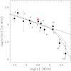 |
Fig. 1 Observed spectrum of the Coma radio halo (black data-points) and the power law (α = 1.22 ± 0.04) that best fits the spectrum at lower frequencies, ν ≤ 1.4 GHz (solid line). Empty points are the data with the SZ correction added, the SZ-decrement is calculated from Planck measurements by adopting an aperture radius =0.48 R500. The dotted line is a synchrotron model assuming a broken power-law energy distribution of the emitting electrons, N(E) ∝ E− δ and ∝ E− (δ + Δδ), at lower and higher energies, with δ = 2.4 and Δδ = 1.6. The dashed line is a synchrotron model assuming a power-law (δ = 2.5) with a high energy cut-off, which occurs for instance in (homogeneous) reacceleration models (see e.g. Schlickeiser et al. 1987). The red point is the flux measured in the high-sensitivity observations at 330 MHz by Brown & Rudnick (2011) within an aperture radius =0.48 R500. |
The radio halo in the Coma cluster is unique in that its spectrum has been measured over almost two decades in frequency (Fig. 1). The observed steepening at high frequencies was used to argue against a hadronic origin of the halo (Schlickeiser et al. 1987; Blasi 2001; Brunetti et al. 2001; Petrosian 2001). Enßlin (2002, E02) first proposed that such a steepening may be caused (at least in part) by the thermal Sunyaev-Zeldovich (SZ) decrement seen in the direction of the cluster. This possibility was further elaborated by PE04, concluding that a simple synchrotron power-law spectrum, with spectral index α = 1.05−1.25, provides a fair description of the observed radio spectrum after taking into account the negative flux bowl due to the SZ effect (see also Enßlin et al. 2011). Other efforts to model the Sunyaev-Zeldovich (SZ) – effect in the Coma cluster, however, concluded that this effect is not significant (Reimer et al. 2004; Donnert et al. 2010). All these attempts used the β-model spatial distribution of the ICM from X-ray observations1, but the differences between the two lines of thought comes essentially from the apertures used to estimate the SZ-decrement.
The Planck satellite has recently obtained resolved and precise measurements of the SZ signal in the Coma cluster (Planck Collaboration 2013, hereafter PIPX). These data strongly reduce the degrees of freedom and uncertainties in the modeling of the SZ contribution and allow a straightforward test of the spectral steepening hypothesis. This is the aim of the present paper.
A ΛCDM cosmology (Ho = 70 km s-1 Mpc-1, Ωm = 0.3, ΩΛ = 0.7) is adopted.
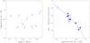 |
Fig. 2 Left: sensitivity to diffuse emission of the observations at different frequencies (rms/beam, scaled to 0.3 GHz with α = 1.22, using an arbitrary scale). Right: radio halo diameters measured from radio maps (using 3σ contours) vs. sensitivity of the observations; for comparison, the empty symbol marks data from the Brown & Rudnick (2011) WSRT observation at 330 MHz. For the Effelsberg data-point at 2.675 GHz (12) we used an upper limit because the size of the halo measured from the contours of the image by T03 is biased high by discrete sources embedded in the halo. |
2. Thermal Sunyaev-Zeldovich effect
The inverse Compton interaction of photons of the Cosmic Microwave Background (CMB) with
hot electrons in the ICM modifies the CMB spectrum, with respect to a blackbody, by a
quantity δFSZ that depends on frequency (see
e.g., Carlstrom et al. 2002, for a review). For low
optical depths this quantity measured on an aperture Ω is
 (1)where the cluster
Compton parameter is
(1)where the cluster
Compton parameter is  (2)l is the
line of sight, and the spectral distortion at the frequency ν is
(2)l is the
line of sight, and the spectral distortion at the frequency ν is
![\begin{equation} f(\nu) = {{x_{\nu}^4 {\rm e}^{x_{\nu}}}\over{({\rm e}^{x_{\nu}} -1)^2}} \left[ {x_{\nu} \over{\tanh(x_{\nu}/2)}} -4 \right] \stackrel{x_{\nu} \rightarrow 0}{\longrightarrow} -2 x_{\nu}^2 , \end{equation}](/articles/aa/full_html/2013/10/aa21402-13/aa21402-13-eq30.png) (3)where
xν = hν/kBTcmb.
At GHz frequencies xν ≪ 1, and the SZ effect
from the ICM in galaxy clusters creates a negative flux bowl on the scale of the clusters.
The flux from radio sources measured by single-dish radio telescopes is that in excess of
the background “zero” level that is determined on larger scales. Once discrete sources are
subtracted appropriately, the resulting flux observed from radio halos in an aperture
ΩH is
Fobs(ν,ΩH) = F(ν,ΩH) + δFSZ(ν,ΩH),
F is relative to the intrinsic emission. The SZ-decrement (negative)
signal, δFSZ, will become comparable to the
flux from the halo at sufficiently high frequencies, leading to an apparent steepening of
the observed spectrum (Liang et al. 2000, E02).
(3)where
xν = hν/kBTcmb.
At GHz frequencies xν ≪ 1, and the SZ effect
from the ICM in galaxy clusters creates a negative flux bowl on the scale of the clusters.
The flux from radio sources measured by single-dish radio telescopes is that in excess of
the background “zero” level that is determined on larger scales. Once discrete sources are
subtracted appropriately, the resulting flux observed from radio halos in an aperture
ΩH is
Fobs(ν,ΩH) = F(ν,ΩH) + δFSZ(ν,ΩH),
F is relative to the intrinsic emission. The SZ-decrement (negative)
signal, δFSZ, will become comparable to the
flux from the halo at sufficiently high frequencies, leading to an apparent steepening of
the observed spectrum (Liang et al. 2000, E02).
3. Implications for the Coma radio halo
In this section we use Planck measurements to calculate the modification of the spectrum of the Coma radio halo at higher frequencies that is caused by the SZ-decrement. Because this correction depends on the aperture over which it is calculated, as well as on the varying radio sensitivities and observed halo sizes in the literature, we used three different approaches to ensure that our results are robust.
-
(i)
We used the halo spectrum from the data compilation from Thierbach et al. (2003, T03) and calculated the SZ decrement in a reference aperture radius that is consistent with those used at the various frequencies in the T03 compilation;
-
(ii)
we used the subset of radio observations for which the actual radial profiles are available to derive the halo spectrum in two fixed aperture radii and self-consistently calculated the SZ decrement within these radii;
-
(iii)
we used the correlation between radio brightness and y-parameter discovered by PIPX to derive the ratio of radio-halo flux and negative SZ flux as a function of frequency and almost independently of the aperture radius.
Before using these different methods for evaluating the SZ contribution, we first discuss the main uncertainties in the radio halo spectrum, in particular the scale size of the halo which is essential for the application of these methods.
Figure 1 shows the observed spectrum from the T03
compilation of data-points2 and the best fit to the
data at lower (≤1.4 GHz) frequencies, a power law with α = 1.22 ± 0.04. We
note that the scatter of the data is larger than expected from the quoted errors (the best
fit has  ),
which suggests systematics that are likely due to the different sensitivities and the
variety of telescope systems used over the past 30 years. To investigate the effects of
sensitivity on the observed halo sizes and fluxes we returned to the original papers used
for Fig. 1. Wherever the information was available, we
show in Fig. 2 (left) the sensitivities to diffuse
emission of the observations at the different frequencies (sensitivities are all scaled to
0.3 GHz using α = 1.22). If we focus on the data at
ν ≤ 1.4 GHz (points 1−11), the comparison between Figs. 1 and 2 (left)
immediately shows that fluxes from higher-sensitivity observations (points 4, 6, 8, 10) are
systematically biased high (about 50% higher) with respect to those derived from the less
sensitive observations (points 1, 5, 9, and 11). This is because better sensitivities allow
one to trace the diffuse emission of the halo to larger distances from the cluster center.
This is clear from Fig. 2 (right), where we show the
diameters of the radio halo that we measured from the 3σ contours in the
published radio maps as a function of the sensitivity. The measured 3σ
diameter (=
),
which suggests systematics that are likely due to the different sensitivities and the
variety of telescope systems used over the past 30 years. To investigate the effects of
sensitivity on the observed halo sizes and fluxes we returned to the original papers used
for Fig. 1. Wherever the information was available, we
show in Fig. 2 (left) the sensitivities to diffuse
emission of the observations at the different frequencies (sensitivities are all scaled to
0.3 GHz using α = 1.22). If we focus on the data at
ν ≤ 1.4 GHz (points 1−11), the comparison between Figs. 1 and 2 (left)
immediately shows that fluxes from higher-sensitivity observations (points 4, 6, 8, 10) are
systematically biased high (about 50% higher) with respect to those derived from the less
sensitive observations (points 1, 5, 9, and 11). This is because better sensitivities allow
one to trace the diffuse emission of the halo to larger distances from the cluster center.
This is clear from Fig. 2 (right), where we show the
diameters of the radio halo that we measured from the 3σ contours in the
published radio maps as a function of the sensitivity. The measured 3σ
diameter (= ,
Rmin and Rmax are the smallest and
largest radii in the map) increases with sensitivity in a way that depends on the brightness
distribution of the radio halo: in Fig. 2 (right) we
also show the behavior expected assuming a radio-brightness distribution of the form
IR ∝ (1 + (r/rc)2)− k,
where rc is the X-ray core radius of Coma,
rc = 10.5 arcmin, and where
k ≃ 0.7 ∗ (3β−1/2), as inferred by
Govoni et al. (2001) (β = 0.75).
This provides a good description of the data; note that points 5 and 11, with the poorest
sensitivities, are both approximated well by the model, but come from very different
frequencies, 151 MHz and 1.38 GHz, respectively.
,
Rmin and Rmax are the smallest and
largest radii in the map) increases with sensitivity in a way that depends on the brightness
distribution of the radio halo: in Fig. 2 (right) we
also show the behavior expected assuming a radio-brightness distribution of the form
IR ∝ (1 + (r/rc)2)− k,
where rc is the X-ray core radius of Coma,
rc = 10.5 arcmin, and where
k ≃ 0.7 ∗ (3β−1/2), as inferred by
Govoni et al. (2001) (β = 0.75).
This provides a good description of the data; note that points 5 and 11, with the poorest
sensitivities, are both approximated well by the model, but come from very different
frequencies, 151 MHz and 1.38 GHz, respectively.
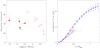 |
Fig. 3 Left: aperture diameter used to measure the radio halo flux as a function of the observing frequency; asteriscs mark single-dish observations. The dashed line marks the representative aperture radius, RH = 0.48 R500, used in our first approach to estimate the SZ-decrement. (Right) Full azimuthal flux profile derived from the Brown & Rudnick (2011) WSRT data (solid, blue) without the quadrant in the west, which is significantly contaminated by the tailed radio source NGC 4869. Errors are dominated by statistical noise at small radii and by the uncertainty in the “zero level” at large radii. The red square marks the total flux and size of the halo from Venturi et al. (1990), while the solid red lines show the integrated flux profile obtained by Govoni et al. (2001) rederived from these same data. The cyan profile is derived from Deiss et al. (1997) at 1.4 GHz and the magenta profile from Pizzo (2010) at 139 MHz. Fluxes at 139 MHz and 1400 MHz are scaled at 330 MHz using a spectrum α = 1.22. |
With a good estimate of the sensitivity dependence, we can now address a key concern, i.e., whether the observed spectral steepening is caused by a lack of sensitivity. For point 12, at 2.675 GHz, the sensitivity is the same as for a number of points from 139 MHz to 1.4 GHz, therefore it is expected to appear on the power-law line (Fig. 1) if there is no spectral steepening. However, it is a factor of ~2 below this line, supporting the case for actual spectral steepening, whether intrinsic or caused by the SZ effect. We also note that the flux of the Coma radio relic measured at 2.675 GHz by T03 is indeed consistent with the power-law shape derived from other observations in the range 151 MHz–4.75 GHz (T03, Fig. 8), adding confidence on the steepening measured by T03 for the halo. The effect of sensitivity on the highest frequency point, 13, can be best assessed by comparison with points 1, 5 and 11, from 30 MHz, 151 MHz and 1380 MHz, respectively, which have a similar sensitivity. The flux of points 1, 5 and 11 is ~20% lower than the power-law line in Fig. 1. A drop of 20% for point 13 does not explain its flux, which is more than a factor of ~3 below the power-law line. We conclude that the spectral steepening at 2.675 GHz and 4.85 GHz is not an observational effect caused by the sensitivity of the observations at the different frequencies.
Systematics in the spectrum might also come from the different procedures used to subtract discrete sources in the halo region. The subtraction becomes critical at higher frequencies where most of the flux in the halo region is associated with discrete sources. The flux at 4.85 GHz of the two brightest sources in the halo region (NGC 4869 and 4874) is known from VLA observations (175 mJy in total, see T03 and Kim 1994), while additional 55 mJy are attributed by T03 to discrete sources in the halo region by using the master-source list of Kim (1994), which also reports spectral indices. Most of the spectral information in Kim (1994) was obtained at frequencies ≤1.6 GHz, therefore the flux of discrete sources may be overestimated if their spectral indices actually steepen at higher frequencies (T03); this would bias the resulting flux of the halo low. We investigated this effect by assuming the typical spectral steepenings between low and high (1.4–4.8 GHz) frequencies that are measured for samples of radio sources, Δα ≤ 0.15 (Kuehr et al. 1981; Helmboldt et al. 2008), and found that the increment of the radio halo flux with respect to that from T03 is <30%, which is lower than the error reported in Fig. 1. Again we conclude that the spectral steepening observed at high frequencies is not driven by obvious observational biases.
As a final step we studied the possible effect caused by the different adopted flux calibration scales, because spectral measurements were taken over a long time-span. The best modern values are presented by Perley & Butler (2013). Using their values for the calibrator 3C 286, we corrected the T03 2675 and 4850 MHz data. This resulted in a reduction of their fluxes by 3.5% and 2.1%, enhancing the steepening by a tiny amount, well within the errors. Most of the other papers summarized by T03 do not explicitly describe their flux scale, although the most common scale in usage was that of Baars et al. (1977). Down to 326 MHz, which is the lowest frequency studied by Perley & Butler, the other literature values would decrease by an average of 1.6%, with the largest decrease being 2.5% for the 608.5 MHz point, producing no significant change in the spectrum3.
We proceed to examine the potential contribution of the SZ effect.
3.1. Method (i)
Our first method of evaluating the SZ contribution involves using the fluxes as reported
in the literature and adopting an appropriate “reference” aperture radius for the
correction. Figure 3 (left) shows the “equivalent
diameter” (defined below) of the regions that is used by the respective authors for flux
measurements, wherever these are available. We deliberately biased our calculations toward
higher SZ contributions by using the (larger) apertures at ν ≤ 1.4 GHz;
at these low frequencies, the SZ decrement is negligible and cannot artificially make the
halo look smaller. In some cases the fluxes were taken from boxes or from complex (non
circular) regions that encompass the scale where diffuse emission is detected, therefore
we define the “equivalent diameter” as  ,
A being the area from which fluxes in the literature were extracted.
,
A being the area from which fluxes in the literature were extracted.
In Fig. 3 we see that for the high-sensitivity points 4, 6, and 10 (139, 330, and 1400 MHz), the aperture radii are consistent with a value of 23′ (=0.48 R500, where R500 = 47 arcmin = 1.3 Mpc, PIPX). The low-sensitivity point 1 at 30 MHz is consistent with this as well. These points with consistent aperture define the power law seen in Fig. 1; the low-sensitivity point 5, at 151 MHz, has a smaller size and is indeed ~20% below the power law in Fig. 1. We therefore adopted 23′ as the radius over which to calculate the SZ correction4.
With this 23′ (0.48 R500) radius, we corrected
for the SZ decrement on scales significantly larger than the observed halo sizes at the
high frequencies (points 12, and 13), and thus we eventually overestimated the actual
effect. From Planck measurements of the Compton parameter
y (PIPX) and from Eqs. (1)–(3), we found
δFSZ = −(1.08 ± 0.05)(ν/GHz)2
mJy. This is about four times lower than that used by PE04 (their Eq. (74)) and about 30%
higher than that used in Donnert et al. (2010). The
main reason for the discrepancy with PE04 is that they calculated the SZ-signal by
integrating Eq. (1) over an excessively large aperture,
 Mpc
(in Eq. (1)
Mpc
(in Eq. (1)  , DA
the angular distance). This corresponds to ~2.75 R500, which
indeed is 5−6 times higher than the radius of the radio halo in the observations of the
T03 compilation (Fig. 3 left)5. Fig. 1 shows the high-frequency
data-points with the SZ correction added (filled symbols). We conclude that the
SZ-decrement is not important: an SZ-decrement about four times larger than that measured
by Planck would be needed to reconcile the data-points at higher
frequency with a power-law spectrum.
, DA
the angular distance). This corresponds to ~2.75 R500, which
indeed is 5−6 times higher than the radius of the radio halo in the observations of the
T03 compilation (Fig. 3 left)5. Fig. 1 shows the high-frequency
data-points with the SZ correction added (filled symbols). We conclude that the
SZ-decrement is not important: an SZ-decrement about four times larger than that measured
by Planck would be needed to reconcile the data-points at higher
frequency with a power-law spectrum.
With this result, we must conclude that the spectral break above 1.4 GHz is intrinsic to the source. We attempted to constrain the magnitude of the break by fitting the data-points in Fig. 1, corrected for the SZ-decrement (adding a flux =1.08(ν/GHz)2 mJy), with a broken power-law with slopes at lower and higher frequencies α and α + Δα. An F-test analysis, using the statistical errors from Fig. 1, constrains Δα > 0.45 (90% confidence level), implying a corresponding break in the spectrum of the emitting electrons Δδ > 0.9. A strong break is also clear from Fig. 1, which shows synchrotron models assuming both a break Δδ = 1.6 (dotted line) and a high-energy cut-off (dashed line). A strong break (or cut-off) in the spectrum of the emitting electrons is thus required by the current data even after correcting for the SZ effect.
3.2. Method (ii)
As a second approach, we directly used the brightness profiles of the radio halo at different frequencies wherever these were available. This avoided problems associated with measurements at better sensitivities, which can be integrated to larger radii. In particular, we constructed new spectra by integrating the lower-frequency fluxes only out to radii of 17.5′ and 13′ (0.37 and 0.27 R500), which correspond to the effective radii at 2.675 and 4.85 GHz, respectively (as in T03). The calculated SZ decrements from the Planck observations are =− 0.82 ± 0.03 and − (0.50 ± 0.02)(ν/GHz)2 mJy, respectively.
In Fig. 4 we show the reconstructed spectrum (SZ-corrected) within these radii. As in method (i), we found that the SZ decrement is negligible and that a correction 4−5 times larger than that implied by Planck measurements would be needed to reconcile the data at 2.675 and 4.85 GHz with the best-fit spectrum obtained at lower frequencies.
We furthermore note that Fig. 4 shows indications for a steepening of the halo spectrum with increasing aperture radius. The best-fit slope obtained using the smallest aperture =13′ (=0.27 R500), α = 1.10 ± 0.01, is smaller than that obtained with an aperture of 17.5′ (=0.37 R500), α = 1.17 ± 0.02, and than the best-fit slope to the TH03 compilation of data, which refer to larger apertures (Sect. 3.1). This qualitatively agrees with the radial spectral steepening of the Coma radio halo that was reported by Giovannini et al. (1993) and Deiss et al. (1997).
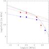 |
Fig. 4 Spectrum of the radio halo extracted within an aperture of 17.5′ (red, 0.37 R500) and 13′ (blue, 0.27 R500). The high-frequency points are corrected for the SZ-decrement measured on the same scales. For comparison the empty symbols mark fluxes measured in the same aperture radius using the Brown & Rudnick (2011) data. Best fits to the low-frequency data are reported as solid lines (same color-code), while the best fit to the T03 compilation (dashed line) and the synchrotron model with the cut-off of Fig. 1 (dot-dashed line) are reported for comparison. |
3.3. Method (iii)
In a third approach we evaluated the importance of the SZ decrement by using the
correlation found by PIPX between the y-signal and the radio flux in a
beam area, F(0.3,Ωb), from recent deep WSRT
observations at 330 MHz (Brown & Rudnick 2011). This is
y = 10-5 × 10(0.86 ± 0.02)(F(0.3,Ωb)/Jy)0.92 ± 0.04,
using a 10-arcmin FWHM beam and measured to a maximum radial distance
~0.8 × R500 ~ 38 arcmin. From Eq. (1), this
point-to-point radio-SZ correlation can be converted into a relation between the
SZ-decrement integrated over a beam area Ωb,
δFSZ(ν,Ωb) = 2(kBT)3f(ν)yΩb/(hc)2,
where Ωb ≃ 9.6 × 10⁻⁶ rad2 and the radio flux
integrated in the same beam. Assuming that the radio halo has an intrinsic power-law
spectrum,
F(ν) ∝ ν− α,
it is 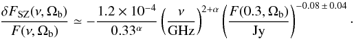 (4)Here the ratio
δFSZ/F
is calculated within a beam area (Ωb = 9.6 × 10⁻⁶ rad2)
and depends on the distance from the cluster center because F, on the
right-hand side of Eq. (4), decreases with distance. However, the quasi-linear scaling
between δFSZ and F makes
this dependence very weak. Indeed, according to Fig. 9 in PIPX,
F(0.3,Ωb) ranges from ~1 Jy in the central
halo regions to ~0.06 Jy in the periphery, implying a maximum variation of
<25% in the ratio
δFSZ/F
as a function of distance. Such a weak dependence allows us to readily also derive a ratio
δFSZ/F
referred to a larger aperture. If we assume the average value of F within
the halo region, F ~ 0.2 Jy (PIPX), we obtain the ratio
δFSZ/F
on the aperture of the halo, ΩH (with
RH ~ 0.85 R500)
(4)Here the ratio
δFSZ/F
is calculated within a beam area (Ωb = 9.6 × 10⁻⁶ rad2)
and depends on the distance from the cluster center because F, on the
right-hand side of Eq. (4), decreases with distance. However, the quasi-linear scaling
between δFSZ and F makes
this dependence very weak. Indeed, according to Fig. 9 in PIPX,
F(0.3,Ωb) ranges from ~1 Jy in the central
halo regions to ~0.06 Jy in the periphery, implying a maximum variation of
<25% in the ratio
δFSZ/F
as a function of distance. Such a weak dependence allows us to readily also derive a ratio
δFSZ/F
referred to a larger aperture. If we assume the average value of F within
the halo region, F ~ 0.2 Jy (PIPX), we obtain the ratio
δFSZ/F
on the aperture of the halo, ΩH (with
RH ~ 0.85 R500)
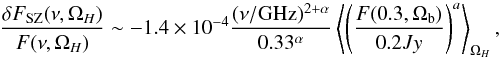 (5)where
a = −0.08 and ⟨ .. ⟩ is a flux-weighted average on
the halo aperture.
(5)where
a = −0.08 and ⟨ .. ⟩ is a flux-weighted average on
the halo aperture.
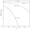 |
Fig. 5 Ratio δFSZ/F as a function of the synchrotron spectral index of the emitted spectrum of the radio halo, assuming a power law F(ν) ∝ ν− α and an average halo flux in a beam area at 330 MHz = 0.2 Jy. Calculations are reported at 1.4, 2.65, 4.85, and 8.45 GHz. Vertical dashed lines mark the synchrotron spectral index of the Coma radio halo derived from data at ν ≤ 1.4 GHz, α = 1.22 ± 0.04. |
The ratio δFSZ/F from Eq. (5) at different frequencies is shown in Fig. 5 assuming different (intrinsic) spectral slopes. Assuming a power law with slope α ~ 1.22, the spectrum of the halo at lower frequencies, we found that the negative signal caused by the SZ-decrement reduces the radio flux at 4.85 GHz by only ≤10%. That is much less than required to substantially affect the shape of the spectrum; for example a reduction of about 75% would be required assuming the T03 data-set (Fig. 1). Therefore, as in the previous cases, we conclude that the steepening induced by the SZ-decrement is negligible.
3.4. Radio halo and SZ-correction on larger scales
The recent WSRT observations (Brown & Rudnick 2011) allow the halo to be firmly traced out to unprecedentely large scales, ~0.8−0.9 R500 radius (Fig. 3 (right)). On small apertures the flux of the halo derived from these observations is consistent with that from Venturi et al. (1990) (Fig. 4), but their higher sensitivity6 allows the detection of more flux. This effect can already be seen on apertures 0.4−0.5 R500 (Fig. 1) and is especially strong on larger scales (Fig. 3 (right)). If we had adopted the ~0.8−0.9 R500 scale for our calculations, the integrated SZ decrement would be about twice as large as that derived above; however, this effect is more than compensated for by the fact that the 330 MHz halo flux integrated on such a large scale is also almost three times higher than in Fig. 1 (Fig. 3, right). Consequently, in this way we would simply re-obtain a similar fractional decrement based on the y-radio correlation (Fig. 5). This is shown in Fig. 6 where the observed data-points at high frequency are compared with a bundle of power-law spectra normalized to the 330 MHz halo flux integrated on an aperture radius =0.85 R500 and corrected for the intervening (negative) SZ-decrement measured by Planck on the same aperture (Fobs(ν,ΩH) = F(ν,ΩH) + δFSZ(ν,ΩH)). We conclude that an intrinsic power-law spectrum with a slope α ~ 1.2−1.3 would produce an observed flux at 4.8 GHz that is 7−8 times higher than that measured by current Effelsberg observations (T03), thus very deep single-dish observations at high frequencies are expected to easily test for the presence of a spectral break in the spectrum of the Coma halo.
As a final remark, we note that our approaches also assumed no influence from the SZ decrement on scales larger than the radio halo scale. To the extent that this is significant, it would eventually bias low the radio “zero” level at high frequencies, and consequently, our procedures would over-estimate the SZ-correction. We expect, however, that this may affect our conclusion only at ≤few percent level.
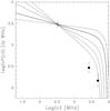 |
Fig. 6 Bundle of power-law spectra, F(ν) ∝ ν− α, with α = 1.1, 1.22, 1.4, 1.55, 1.7 normalized to the flux of the radio halo derived from Brown & Rudnick (2011) WSRT data using an aperture radius RH = 0.85 R500. Models are corrected for the SZ-decrement (Fobs(ν,ΩH) = F(ν,ΩH) + δFSZ(ν,ΩH), Sect. 2) measured on the same aperture radius. The observed high-frequency points are taken from T03. |
4. Conclusions
The spectra of radio halos are important probes of the underlying mechanisms for the acceleration of the electrons responsible for the radio emission. The spectrum of the Coma radio halo shows a steepening at higher frequencies. This has triggered an on-going debate on the possibility that this steepening is not intrinsic to the emitted radiation, but it is caused by the intervening SZ effect with the thermal ICM. The recent Planck data (PIPX) allow for a correct evaluation of this effect.
Using Planck results, we have shown that the negative signal caused by the SZ decrement does not produce a significant effect on the shape of the spectrum of the Coma radio halo.
The spectral information of the Coma halo comes from heterogeneous observations in the past 30 years. For this reason, before evaluating the potential effect of the SZ-effect, we have discussed the main uncertainties on the halo spectrum that derive from the different sensitivities of the observations at different frequencies, from the different apertures used to measure the flux of the halo, and from subtracting discrete sources embedded in the halo region. We showed that the different sensitivities of the observation can explain the large ± 30% scattering of the data-points observed in the global spectrum of the halo collected by T03. However, we also showed that neither the different sensitivity of the observations (and the aperture radius of the halo), nor the subtraction of discrete sources can naturally explain the steepening of the halo spectrum observed at higher frequencies.
We examined the potential contribution of the SZ-effect to the observed steepening using three complementary approaches to ensure that our results are robust.
With the first two methods we measured the SZ-decrement by self-consistently adopting the aperture radii used for flux measurements of the radio halo at the different frequencies. First we adopted the global compilation of data-points from T03 and a radius =23 arcmin which is consistent with the aperture used to measure the halo flux in the most sensitive observations, between 30 MHz and 1.4 GHz. We derived an SZ-decrement =− 1.08(ν/GHz)2 mJy, which is about four times smaller than that required to explain the observed steepening. Second we used the available brightness profiles of the halo at 139, 330, and 1400 MHz to derive the spectrum of the halo within two fixed apertures, =17.5 and 13 arcmin, which correspond to the effective radius of the regions where the halo is detected at higher frequencies, 2.675 and 4.85 GHz, respectively. In this case the flux of the halo between 139 and 1400 MHz is lower than that in the T03 compilation, but the SZ-signal measured by Planck within these apertures also decreases significantly and is about 4−5 times weaker than that required to explain the steepening of the spectrum measured within the same apertures. As a third complementary approach we used the (almost) scale-independent correlation between y and the 330 MHz halo’s flux within a beam-aperture discovered by PIPX. From this correlation we derived the ratio of the SZ-decrement and the radio flux of the halo, δFSZ/F, and showed that this is very low. In particular, by assuming a spectral index of the halo α = 1.2−1.3 the ratio is δFSZ/F ≤ 10% at 4.85 GHz, whereas it should be ≥70% to explain the steepening observed by T03.
Consequently, based on current radio data, our analysis demonstrated that an intrinsic spectral break, or cut-off, is required in the energy distribution of the electrons that generate the radio halo.
It is important to note, however, that the spectral analysis presented here does not tell the whole story of Coma radio spectrum. The recent very high sensitivity observations by Brown & Rudnick (2011) showed that most of the total flux at 330 MHz is emitted beyond a radius of 20−25 arcmin, implying that the halo flux is significantly higher than previously thought. The upcoming LOFAR observations at low frequencies and more sensitive single-dish measurements at high frequencies have the potential of detecting the halo on larger scales and will be essential for evaluating the global spectral shape of the halo and possible spectral variations with radius. For instance, we also showed that future deep observations with single dishes at 5 GHz are expected to measure a halo flux on a 40 arcmin aperture radius that is predicted to be ~7−8 times higher than currently measured if a spectral steepening is absent, thus providing a complementary test to our present findings.
We also add WSRT data at 139 MHz (Pizzo 2010).
Here we ignore point 7, at 430 MHz (Hanisch 1980), which shows a larger radius, to have a consistent aperture within which the fluxes are measured. However, including it has no effect on the spectral fit (Fig. 1). In addition, we note that although its larger radius should have led to a higher flux, oversubtraction of point sources in the central region of the halo, which led to a bowl in the Hanisch (1980) map (Fig. 1c in Hanisch 1980), resulted in fluxes consistent with the 23′ power law.
Within this large aperture we found that the SZ-decrement measured by Planck
is ≃ −3.7(ν/GHz)2 mJy. This is
slightly smaller than the PE04 value, which was calculated using X-ray data, assuming an
isothermal (kT = 8.2 keV) and spherical cluster with the spatial
distribution of the gas density given by the the extrapolation of the beta-model to
Mpc distances.
These observations are ~4−5 times deeper (brightness sensitivity) than those in Venturi et al. (1990).
Acknowledgments
We thank the referee for useful comments and R. Pizzo and T.Venturi for providing useful information on their observations. L. R. acknowledges support from the U.S. National Science Foundation, under grant AST-1211595 to the University of Minnesota. J.D. acknowledges support by FP7 Marie Curie programme “People” of the European Union. K.D. acknowledges the support by the DFG Cluster of Excellence “Origin and Structure of the Universe”.
References
- Ackermann, M., Ajello, M., Allafort, A., et al. 2010, ApJ, 717, L71 [NASA ADS] [CrossRef] [Google Scholar]
- Baars, J., Genzel, G., Pauliny-Toth, I., & Witzel, A. 1977, A&A, 61, 99 [NASA ADS] [Google Scholar]
- Beresnyak, A., Xu, H., Li, H., & Schlickeiser, R. 2013, ApJ, 771, 131 [NASA ADS] [CrossRef] [Google Scholar]
- Blasi, P. 2001, Astropart. Phys., 15, 223 [Google Scholar]
- Blasi, P., & Colafrancesco, S. 1999, Astropart. Phys., 12, 169 [NASA ADS] [CrossRef] [Google Scholar]
- Brown, S., & Rudnick, L. 2011, MNRAS, 412, 2 [NASA ADS] [CrossRef] [Google Scholar]
- Brunetti, G. 2004, JKAS, 37, 493 [NASA ADS] [CrossRef] [Google Scholar]
- Brunetti, G., & Blasi, P. 2005, MNRAS, 363, 1173 [NASA ADS] [CrossRef] [Google Scholar]
- Brunetti, G., & Lazarian, A., 2007, MNRAS, 378, 245 [NASA ADS] [CrossRef] [Google Scholar]
- Brunetti, G., & Lazarian, A. 2011, MNRAS, 410, 127 [NASA ADS] [CrossRef] [Google Scholar]
- Brunetti, G., Setti, G., Feretti, L., & Giovannini, G. 2001, MNRAS, 320, 365 [NASA ADS] [CrossRef] [Google Scholar]
- Brunetti, G., Giacintucci, S., Cassano, R., et al. 2008, Nature, 455, 944 [NASA ADS] [CrossRef] [Google Scholar]
- Brunetti, G., Blasi, P., Reimer, O., et al. 2012, MNRAS, 426, 956 [NASA ADS] [CrossRef] [Google Scholar]
- Buote, D. A. 2001, ApJ, 553, L15 [NASA ADS] [CrossRef] [Google Scholar]
- Carlstrom, J. E., Holder, G. P., & Reese, E. D. 2002, ARA&A, 40, 643 [NASA ADS] [CrossRef] [Google Scholar]
- Cassano, R., & Brunetti, G. 2005, MNRAS, 357, 1313 [NASA ADS] [CrossRef] [Google Scholar]
- Cassano, R., Brunetti, G., Venturi, T., et al. 2008, A&A, 480, 687 [NASA ADS] [CrossRef] [EDP Sciences] [Google Scholar]
- Cassano, R., Ettori, S., Giacintucci, S., et al. 2010, ApJ, 721, L82 [NASA ADS] [CrossRef] [Google Scholar]
- Cassano, R., Ettori, S., Brunetti, G., et al. 2013, ApJ, in press [arXiv:1306.4379] [Google Scholar]
- Deiss, B. M., Reich, W., Lesch, H., & Wielebinski, R. 1997, A&A, 321, 55 [NASA ADS] [Google Scholar]
- Dennison, B. 1980, ApJ, L239 [Google Scholar]
- Donnert, J., Dolag, K., Brunetti, G., Cassano, R., & Bonafede, A. 2010, MNRAS, 401, 47 [NASA ADS] [CrossRef] [Google Scholar]
- Enßlin, T. A. 2002, A&A, 396, L17 (E02) [NASA ADS] [CrossRef] [EDP Sciences] [Google Scholar]
- Enßlin, T., Pfrommer, C., Miniati, F., & Subramanian, K. 2011, A&A, 527, A99 [NASA ADS] [CrossRef] [EDP Sciences] [Google Scholar]
- Fujita, Y., Takizawa, M., & Sarazin, C. L. 2003, ApJ, 584, 190 [NASA ADS] [CrossRef] [Google Scholar]
- Giovannini, G., Feretti, L., Venturi, T., Kim, K.-T., & Kronberg, P. P. 1993, ApJ, 406, 399 [NASA ADS] [CrossRef] [Google Scholar]
- Giovannini, G., Tordi, M., & Feretti, L. 1999, New A, 4, 141 [Google Scholar]
- Govoni, F., Feretti, L., Giovannini, G., et al. 2001, A&A, 376, 803 [NASA ADS] [CrossRef] [EDP Sciences] [Google Scholar]
- Govoni, F., Markevitch, M., Vikhlinin, A., et al. 2004, ApJ, 605, 695 [NASA ADS] [CrossRef] [Google Scholar]
- Hanisch, R. 1980, AJ, 85, 1565 [NASA ADS] [CrossRef] [Google Scholar]
- Helmboldt, J. F., Kassim, N. E., Cohen, A. S., Lane, W. M., & Lazio, T. J. 2008, ApJS, 174, 313 [NASA ADS] [CrossRef] [Google Scholar]
- Liang, H., Hunstead, R.W., Birkinshaw, M., & Andreani, P. 2000, ApJ, 544, 686 [NASA ADS] [CrossRef] [Google Scholar]
- Jeltema, T. E., & Profumo, S. 2011, ApJ, 728, 53 [NASA ADS] [CrossRef] [Google Scholar]
- Kale, R., & Dwarakanath, K. S. 2010, ApJ, 718, 939 [NASA ADS] [CrossRef] [Google Scholar]
- Kempner, J. C., & Sarazin, C. L. 2001, ApJ, 548, 639 [NASA ADS] [CrossRef] [Google Scholar]
- Keshet, U., & Loeb, A. 2010, ApJ, 722, 737 [NASA ADS] [CrossRef] [Google Scholar]
- Kuehr, H., Witzel, A., Pauliny-Toth, I. I. K., & Nauber, U. 1981, A&AS, 45, 367 [NASA ADS] [Google Scholar]
- Macario, G., Venturi, T., Brunetti, G., et al. 2010, A&A, 517, A43 [NASA ADS] [CrossRef] [EDP Sciences] [Google Scholar]
- Macario, G., Venturi, T., Intema, H. T., et al. 2013, A&A, 551, A141 [NASA ADS] [CrossRef] [EDP Sciences] [Google Scholar]
- Orru’, E., Murgia, M., Feretti, L., et al. 2007, A&A, 467, 943 [NASA ADS] [CrossRef] [EDP Sciences] [Google Scholar]
- Perley, R., & Butler, B. 2013 ApJSS, 204, 19 [Google Scholar]
- Petrosian, V. 2001, ApJ, 557, 560 [NASA ADS] [CrossRef] [Google Scholar]
- Pfrommer, C., & Enßlin, T. A. 2004, A&A, 413, 17 (PE04) [NASA ADS] [CrossRef] [EDP Sciences] [Google Scholar]
- Pizzo, R. 2010, Ph.D. Thesis, Groningen University [Google Scholar]
- Planck Collaboration 2013, A&A, 554, A140 (PIPX) [NASA ADS] [CrossRef] [EDP Sciences] [Google Scholar]
- Reimer, A., Reimer, O., Schlickeiser, R., & Iyudin, A. 2004, A&A 424, 773 [NASA ADS] [CrossRef] [EDP Sciences] [Google Scholar]
- Schlickeiser, R., Sievers, A., & Thiemann, H. 1987, A&A, 182, 21 [NASA ADS] [Google Scholar]
- Thierbach, M., Klein, U., & Wielebinski, R. 2003, A&A, 397, 53 (T03) [NASA ADS] [CrossRef] [EDP Sciences] [Google Scholar]
- van Weeren, R. J., Röttgering, H. J. A., Rafferty, D. A., et al. 2012, A&A, 543, A43 [NASA ADS] [CrossRef] [EDP Sciences] [Google Scholar]
- Venturi, T., Giovannini, G., & Feretti, L. 1990, AJ, 99, 1381 [NASA ADS] [CrossRef] [Google Scholar]
- Venturi, T., Giacintucci, S., Dallacasa, D., et al. 2008, A&A, 484, 327 [NASA ADS] [CrossRef] [EDP Sciences] [Google Scholar]
- Venturi, T., Giacintucci, S., Dallacasa, D., et al. 2013, A&A, 551, A24 [NASA ADS] [CrossRef] [EDP Sciences] [Google Scholar]
All Figures
|
Fig. 1 Observed spectrum of the Coma radio halo (black data-points) and the power law (α = 1.22 ± 0.04) that best fits the spectrum at lower frequencies, ν ≤ 1.4 GHz (solid line). Empty points are the data with the SZ correction added, the SZ-decrement is calculated from Planck measurements by adopting an aperture radius =0.48 R500. The dotted line is a synchrotron model assuming a broken power-law energy distribution of the emitting electrons, N(E) ∝ E− δ and ∝ E− (δ + Δδ), at lower and higher energies, with δ = 2.4 and Δδ = 1.6. The dashed line is a synchrotron model assuming a power-law (δ = 2.5) with a high energy cut-off, which occurs for instance in (homogeneous) reacceleration models (see e.g. Schlickeiser et al. 1987). The red point is the flux measured in the high-sensitivity observations at 330 MHz by Brown & Rudnick (2011) within an aperture radius =0.48 R500. |
| In the text | |
|
Fig. 2 Left: sensitivity to diffuse emission of the observations at different frequencies (rms/beam, scaled to 0.3 GHz with α = 1.22, using an arbitrary scale). Right: radio halo diameters measured from radio maps (using 3σ contours) vs. sensitivity of the observations; for comparison, the empty symbol marks data from the Brown & Rudnick (2011) WSRT observation at 330 MHz. For the Effelsberg data-point at 2.675 GHz (12) we used an upper limit because the size of the halo measured from the contours of the image by T03 is biased high by discrete sources embedded in the halo. |
| In the text | |
|
Fig. 3 Left: aperture diameter used to measure the radio halo flux as a function of the observing frequency; asteriscs mark single-dish observations. The dashed line marks the representative aperture radius, RH = 0.48 R500, used in our first approach to estimate the SZ-decrement. (Right) Full azimuthal flux profile derived from the Brown & Rudnick (2011) WSRT data (solid, blue) without the quadrant in the west, which is significantly contaminated by the tailed radio source NGC 4869. Errors are dominated by statistical noise at small radii and by the uncertainty in the “zero level” at large radii. The red square marks the total flux and size of the halo from Venturi et al. (1990), while the solid red lines show the integrated flux profile obtained by Govoni et al. (2001) rederived from these same data. The cyan profile is derived from Deiss et al. (1997) at 1.4 GHz and the magenta profile from Pizzo (2010) at 139 MHz. Fluxes at 139 MHz and 1400 MHz are scaled at 330 MHz using a spectrum α = 1.22. |
| In the text | |
|
Fig. 4 Spectrum of the radio halo extracted within an aperture of 17.5′ (red, 0.37 R500) and 13′ (blue, 0.27 R500). The high-frequency points are corrected for the SZ-decrement measured on the same scales. For comparison the empty symbols mark fluxes measured in the same aperture radius using the Brown & Rudnick (2011) data. Best fits to the low-frequency data are reported as solid lines (same color-code), while the best fit to the T03 compilation (dashed line) and the synchrotron model with the cut-off of Fig. 1 (dot-dashed line) are reported for comparison. |
| In the text | |
|
Fig. 5 Ratio δFSZ/F as a function of the synchrotron spectral index of the emitted spectrum of the radio halo, assuming a power law F(ν) ∝ ν− α and an average halo flux in a beam area at 330 MHz = 0.2 Jy. Calculations are reported at 1.4, 2.65, 4.85, and 8.45 GHz. Vertical dashed lines mark the synchrotron spectral index of the Coma radio halo derived from data at ν ≤ 1.4 GHz, α = 1.22 ± 0.04. |
| In the text | |
|
Fig. 6 Bundle of power-law spectra, F(ν) ∝ ν− α, with α = 1.1, 1.22, 1.4, 1.55, 1.7 normalized to the flux of the radio halo derived from Brown & Rudnick (2011) WSRT data using an aperture radius RH = 0.85 R500. Models are corrected for the SZ-decrement (Fobs(ν,ΩH) = F(ν,ΩH) + δFSZ(ν,ΩH), Sect. 2) measured on the same aperture radius. The observed high-frequency points are taken from T03. |
| In the text | |
Current usage metrics show cumulative count of Article Views (full-text article views including HTML views, PDF and ePub downloads, according to the available data) and Abstracts Views on Vision4Press platform.
Data correspond to usage on the plateform after 2015. The current usage metrics is available 48-96 hours after online publication and is updated daily on week days.
Initial download of the metrics may take a while.