© ESO, 2013

1. Introduction

In the standard theory of big bang nucleosynthesis (SBBN), given the number of light neutrino species, the abundances of light elements D, ³He, ⁴He and ⁷Li depend only on one cosmological parameter, the baryon-to-photon number ratio η, which is related to the baryon density parameter Ω_b, the present ratio of the baryon mass density to the critical density of the Universe, by the expression 10¹⁰η = 273.9 Ω_bh², where h = H₀/100 km s^-1 Mpc^-1 and H₀ is the present value of the Hubble parameter (Steigman 2005, 2012).

Because of the strong dependence of the D/H abundance ratio on Ω_bh², deuterium is the best-suited light element for determining the baryon mass fraction. Its abundance can accurately be measured in high-redshift low-metallicity QSO Lyα absorption systems. Although the data are still scarce − there are only ten absorption systems for which such a D/H measurement has been carried out (Pettini & Cooke 2012) – the measurements appear to converge to a mean primordial value D/H ~ (2.5−2.9) × 10^-5, which corresponds to Ω_bh² ~ 0.0222−0.0223 (Iocco et al. 2009; Noterdaeme et al. 2012; Pettini & Cooke 2012). This estimate of Ω_bh² agrees excellently with the value of 0.0221−0.0222 obtained from studies of the fluctuations of the cosmic microwave background (CMB) with WMAP and Planck (Keisler et al. 2011, Planck Collaboration 2013).

While deuterium is sufficient to derive the baryonic mass density from BBN, accurate measurements of the primordial abundances of at least two different relic elements are required to verify the consistency of SBBN. The primordial abundance of ⁴He can in principle be derived accurately from observations of the helium and hydrogen emission lines from low-metallicity blue compact dwarf (BCD) galaxies, which have undergone little chemical evolution. Several groups have used this technique to derive the primordial ⁴He mass fraction Y_p. The most recent determinations of Y_p have resulted in high values of 0.2565 ± 0.0060 (2σ) (Izotov & Thuan 2010) and 0.2534 ± 0.0083 (1σ) (Aver et al. 2012), implying deviations from the SBBN and existence of additional types of neutrino species such as sterile neutrinos. However, taking into account large statistical and systematic errors in the Y_p determination, one can conclude that these latest determinations of Y_p are broadly (at the 3σ level) consistent with the prediction of SBBN, Y_p = 0.2477 ± 0.0001 (Ade et al. 2013). Although ⁴He is not a sensitive baryometer (Y_p depends only logarithmically on the baryon density), its primordial abundance depends much more sensitively on the expansion rate of the Universe and thus on any small deviation from SBBN, than that of the other primordial light elements (Steigman 2006).

However, to detect small deviations from SBBN and make cosmological inferences, Y_p has to be determined to a level of accuracy of less than one percent. This is not an easy task. While it is relatively straightforward to derive the helium abundance in an H ii region with an accuracy of 10 percent if the spectrum is adequate, gaining a factor of several in accuracy requires many conditions to be met. First, the observational data have to be of good quality and should constitute a large sample to reduce statistical uncertainties in the determination of Y_p. This has been the concern of studies conducted for instance by Izotov et al. (1994, 1997), Izotov & Thuan (1998b, 2004), who obtained 93 high signal-to-noise spectra of low-metallicity extragalactic H ii regions, which includes a total of 86 H ii regions in 77 galaxies (the HeBCD sample, see Izotov & Thuan 2004). Furthermore, Izotov et al. (2009, 2011b) and Guseva et al. (2011) collected a sample of 75 spectra of low-metallicity H ii regions in different galaxies observed with the Very Large Telescope (VLT) (VLT sample). Finally, 1442 high-quality spectra of low-metallicity H ii regions were extracted from the Sloan Digital Sky Survey (SDSS) (SDSS sample). They were selected from the SDSS Data Release 7 (DR7), as were those with the [O iii] λ4363 emission line measured with an accuracy better than 25%. Additionally, all strongest He i emission lines in the optical range, λ3889, λ4471, λ5876, λ6678, and λ7065, had to be present in the spectrum and measured with good accuracy. Part of the SDSS sample containing ~800 galaxies with the highest Hβ luminosities, was discussed by Izotov et al. (2011b). In total, the HeBCD, VLT and SDSS samples together constitute by far the largest sample of high-quality spectra assembled to investigate the problem of the primordial helium abundance. Because of greatly increased samples it turns out that the accuracy of the determination of the primordial ⁴He abundance is limited at present more by systematic uncertainties and biases than by statistical errors.

Different empirical methods have been used to derive physical conditions and element abundances and to convert the observed He i emission line intensities to a ⁴He abundance (e.g. Izotov et al. 1994, 1997; Izotov & Thuan 2010; Peimbert et al. 2007; Aver et al. 2010, 2011, 2012). All of them use fits of different processes (e.g. Izotov et al. 2006), including the fits of He i and H emissivities and different effects that result in observed line intensities that are different from their recombination values. There are many known effects we need to correct for to transform the observed He i line intensities into a ⁴He abundance. Neglecting or misestimating them may lead to systematic errors in the Y_p determination that are larger than the statistical errors. These effects are (1) reddening; (2) underlying stellar absorption in the He i lines; (3) collisional excitation of the He i lines that result in intensities different from their recombination values; (4) fluorescence of the He i lines, which also result in intensities different from their recombination values; (5) collisional excitation of the hydrogen lines; (6) possible departures from case B in the emissivities of H and He i lines; (7) the temperature structure of the H ii region; and (8) its ionisation structure. The role of each of these effects is discussed for instance by Izotov et al. (2007).

Most of the systematic effects are taken into account in the most recent papers (e.g. Izotov et al. 2007; Izotov & Thuan 2010; Peimbert et al. 2007; Aver et al. 2010, 2012). However, one important problem remains. While corrections for many effects were obtained with photoionised H ii region models (e.g. with CLOUDY, Ferland et al. 1998, 2013), the overall procedure for determining the ⁴He abundance has never been tested on photoionisation models. Since a photoionisation code such as CLOUDY takes into account all the processes affecting the He i line intensities (radiation transfer, ionisation and recombination processes, heating and cooling, collisional and fluorescence excitation, etc.), it produces in principle model H ii regions that should be close to real H ii regions. Of course, the gas density distributions, the distribution of the ionising stars and their spectral energy distributions are simplified with respect to reality, but how could one trust a method that does not recover the correct helium abundance used to compute these models when treating the models in the same way as observations are treated? Of course, such an exercise needs to be made using exactly the same atomic ingredients as are implied in CLOUDY calculations, since the objective is to judge the method itself and, if necessary, improve it.

In the present paper we test the empirical method developed in a number of our papers (e.g. Izotov et al. 1994, 1997, 2007; Izotov & Thuan 2010) using a grid of photoionised H ii region models calculated with version v13.01 of the CLOUDY code (Ferland et al. 2013). In Sect. 2 we describe our grid of CLOUDY photoionisation models. The fits of new emissivities for 32 He i emission lines tabulated by Porter et al. (2013) are discussed in Sect. 3. Ionisation correction factors for He and their fits are obtained in Sect. 4. We consider the non-recombination excitation of hydrogen in Sect. 5. In Sect. 6 we examine how well our empirical method recovers the ⁴He abundance with which the photoionisation models were constructed, and update it to improve the results. In Sect. 7 we discuss the additional systematic effects that appear in real H ii regions, describe our sample of low-metallicity H ii regions, apply our updated empirical method to determine the ⁴He abundance in these objects and justify the linear regressions used for the primordial ⁴He abundance determination. In Sect. 8 we present the linear regressions Y – O/H and derive the primordial ⁴He mass fraction Y_p. Cosmological implications of the derived Y_p are discussed in Sect. 9. In particular, we derive the effective number of neutrino species N_eff. Section 10 summarises our main results.

2. Grid of photoionisation CLOUDY models

Using version v13.01 of CLOUDY code (Ferland et al. 2013), we calculated a grid of 576 homogeneous spherical ionisation-bounded H ii region models with parameters shown in Table 1, which cover the entire range of parameters in real low-metallicity H ii regions used for the ⁴He abundance determination. In particular, the range of oxygen abundances is 12 + log    O/H   =   7.3−8.3. The abundances of other heavy elements relative to oxygen are kept constant corresponding to typical values obtained for low-metallicity emission-line galaxies (e.g. Izotov et al. 2006). The ⁴He abundance in all models, however, is the same with Y = 0.254. We also included dust, scaling it according to the oxygen abundance. The characteristics adopted for the dust are those offered by CLOUDY as “Orion nebula dust”. For all the models we used the “iterate” option.

We adopted three values of the number of ionising photons Q and the shape of the ionising radiation spectrum corresponding to the Starburst99 model with the ages of 1.0, 2.0, 3.5, and 4.0 Myr and different metallicities. Thus, for 12 + log O/H = 7.3 and 7.6 we adopted Starburst99 models with a heavy-element mass fraction Z = 0.001, for those with 12 + log O/H = 8.0 models with Z = 0.004, and for those with 12 + log O/H = 8.3 models with Z = 0.008. All Starburst99 models were calculated with the stellar tracks from Meynet et al. (1994) and the Hillier & Miller (1998) and Pauldrach et al. (2001) stellar atmosphere set. We also varied the log of the volume-filling factor f between −0.5 and −2.0 to obtain CLOUDY models with different ionisation parameters. For the subsequent analysis, out of the 576 H ii region models we selected the 363 that had a volume-averaged ionisation parameter of log U between −3 and −2. This range of log U is typical for the real high-excitation low-metallicity H ii regions used for the ⁴He abundance determination.

Our range of the number density N_e = 10−10³ cm^-3, which was kept constant along the H ii region radius, covers the whole range expected for the extragalactic H ii regions used for the ⁴He abundance determination.

Additionally, to study the effect of density inhomogeneities, we calculated two sets of models, each consisting of the 192 H ii region models with parameters from Table 1 (excluding N_e). The density in the first set of inhomogeneous models has a Gaussian distribution along the radius r according to ${\mathit{N}}_{\mathrm{e}}\mathrm{\left(}\mathit{r}\mathrm{\right)}\mathrm{=}{\mathit{N}}_{\mathrm{e}}\mathrm{\left(}\mathrm{0}\mathrm{\right)}\exp \left[\mathrm{-}\frac{{\mathit{r}}^{\mathrm{2}}}{\mathrm{(}\mathrm{30}\hspace{0.17em}\mathrm{pc}{\mathrm{)}}^{\mathrm{2}}}\right]\mathit{,}$(1)where N_e(0) = 10³ cm^-3. The volume-averaged log U in 86 H ii region models out of 192 H ii region models with Gaussian density distribution is in the range −3−−2.

The density in the second set of 192 inhomogeneous models was varied periodically with radius in the range N_e = 10−10² cm^-3. A volume-averaged log U in 117 H ii region models out of 192 H ii region models with periodic density distribution is in the range −3−−2. Thus, the total number of the models we used for our analysis is 363 + 86 + 117 = 566.

In our comparison, we used CLOUDY-calculated emission-line intensities as the input parameters for our empirical method.

3. He I emissivities

3.1. Emissivity fits

In our empirical method we used the latest set of He i emissivities tabulated by Porter et al. (2013) for a wide range of the electron temperature T_e and the electron number density N_e. Similar to Porter et al. (2007), we first fitted tabulated data for 32 He i emission lines in the low-density limit with negligible collisional excitation, $\frac{\mathrm{4}\mathit{\pi }{\mathit{j}}_{\mathit{\lambda }}}{{\mathit{N}}_{\mathrm{e}}{\mathit{N}}_{{\mathrm{He}}^{\mathrm{+}}}}\mathrm{=}\left[\mathit{a}\mathrm{+}\mathit{b}\mathrm{(}\ln {\mathit{T}}_{\mathrm{e}}{\mathrm{)}}^{\mathrm{2}}\mathrm{+}\mathit{c}\ln {\mathit{T}}_{\mathrm{e}}\mathrm{+}\frac{\mathit{d}}{\ln {\mathit{T}}_{\mathrm{e}}}\right]{\mathit{T}}_{\mathrm{e}}^{-1}\mathrm{\times }{\mathrm{10}}^{-25}\mathit{,}$(2)where the emissivity 4πj_λ/N_eN_He⁺ is in ergs cm³ s^-1. The coefficients of the fits for the electron temperature range T_e = 5000−25   000 K are shown in Table 2. These fits reproduce tabulated data for low N_e = 10 cm^-3 with an accuracy of better than 0.1%.

To fit the ratio of collisional to recombination excitation of He i emission lines we used the equation (Kingdon & Ferland 1995) 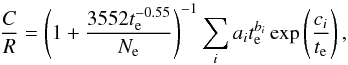$\frac{\mathit{C}}{\mathit{R}}\mathrm{=}{\left(\mathrm{1}\mathrm{+}\frac{\mathrm{3552}{\mathit{t}}_{\mathrm{e}}^{-0.55}}{{\mathit{N}}_{\mathrm{e}}}\right)}^{-1}\sum _{\mathit{i}}{\mathit{a}}_{\mathit{i}}{\mathit{t}}_{\mathrm{e}}^{{\mathit{b}}_{\mathit{i}}}\exp \left(\frac{{\mathit{c}}_{\mathit{i}}}{{\mathit{t}}_{\mathrm{e}}}\right)\mathit{,}$(3)where t_e is T_e/10   000, and i is an index that varies from 1 to 9. The coefficients of the fits for 32 He i emission lines are given in Table 3. We note, however, that we use nine terms in Eq. (3), while Porter et al. (2007) used six terms at most. To find the total emissivity of a given line, we simply multiplied the result obtained from Eq. (2) by the quantity 1 + C/R obtained in Eq. (3). In Fig. 1 we compare our fits of emissivities including collisional excitation for some of the brightest He i emission lines for the electron number densities N_e = 10, 10², and 10³ cm^-3 and the entire range of electron temperatures T_e with those tabulated by Porter et al. (2013). It is seen that the accuracy of our fits is similar to or better than 1% for the electron temperatures T_e = 10   000−20   000 K and entire range of N_e, which are the ranges of T_e and N_e in H ii regions used for the ⁴He abundance determination.

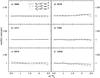Fig. 1 Comparison of calculated and fitted emissivities of the strongest He i emission lines for three values of the electron number densities Ne = 10, 102, and 103 cm-3. Collisional excitation is taken into account.

3.2. Calculating the He I emission-line intensities in CLOUDY

Now we analyse the calculation of He i line intensities in CLOUDY with respect to the He i emissivities. CLOUDY outputs include H and He i emission-line intensities calculated under different assumptions: 1) case A; 2) case A, including collisional contribution; 3) case B; 4) case B, including collisional contribution, etc. One of the CLOUDY outputs are the He i line intensities calculated taking into account all detailed physics regarding collisional transitions, radiative transfer, etc. This is the “predicted line intensity with all processes included” in the CLOUDY output. One would expect that for a low-density ionisation-bounded H ii region these calculated He i emission-line intensities would be close to the CLOUDY output recombination case B intensities. In Fig. 2 we show the ratios of CLOUDY line intensities calculated with taking into account all processes to CLOUDY case B intensities for some important He i emission lines in the models with the electron number density N_e = 10 cm^-3. The collisional excitation of He i emission lines at this low N_e is very low. It is highest for the λ7065 emission line and does not exceed 1.5% of the recombination intensity.

Fig. 2 Ratio of the CLOUDY-calculated intensities with all processes included to CLOUDY case B intensities for several brightest He i emission lines as a function of the oxygen abundance for the models with low electron number density Ne = 10 cm-3. For clarity only models with log Q(H) = 53 are shown.

The only known mechanism that may cause line intensities to deviate from their recombination values in Fig. 2 is the fluorescent excitation due to the non-negligible optical depth for the He i λ3889 emission line. Two emission lines, He i λ3889 and λ7065, are the most sensitive to the fluorescent excitation. However, the optical depth of the He i λ3889 emission line in the models considered in Fig. 2 is small, ≲0.1. Therefore, the effect of fluorescent excitation is low in the considered models with N_e = 10 cm^-3. It is seen in Fig. 2 that the intensities of He iλ3889 and λ7065 emission lines with “all processes included” are close to the case B intensities.

Similarly, the calculated intensity of the singlet He i λ5016 emission line is close to the case B value, indicating that the considered models have high optical depths in the resonance transitions from the ground level of the singlet He i state (e.g., the optical depth of the λ584 line in the CLOUDY output is ≳10⁵), closely corresponding to the case B.

On the other hand, the intensities of two important lines, λ5876 and λ6678, calculated with “all processes included” are higher by ~6%−7% than the case B values, which is difficult to understand, because both lines are less affected by collisional and fluorescent excitation than the λ3889 and λ7065 lines. The same effect to a lesser extent is also present for the λ4471 line. It is likely that there is a problem in the computation of the He i emission line intensities in version v13.01 of the CLOUDY code. Therefore, we did not use the CLOUDY He i intensities with “all processes included” in our subsequent analysis for all He i emission lines. Instead, we adopted the CLOUDY He i case B intensities enhanced by collisions.

4. Ionisation correction factors for He

For our comparison of the empirical method with the CLOUDY models we also needed to take into account the ionisation structure of the H ii region in the empirical method. The He⁺ zone can be slightly larger or slightly smaller than the H⁺ zone, depending on the spectral energy distribution of the ionising radiation. This effect was taken into account in our previous work (e.g. Izotov et al. 2007) by introducing the ionisation correction factor ICF(He) as a function of the excitation parameter x = O²⁺/(O⁺+O²⁺). The CLOUDY output allows us to obtain the exact value of ICF(He), which is equal to x(H⁺)/(x(He⁺)+x(He²⁺)), where x stands for volume-integrated ionic fractions. We fitted these ICF(He) (colour symbols in Fig. 3) for four values of 12 + log O/H = 7.3, 7.6, 8.0 and 8.3 and for four values of the starburst age 1.0, 2.0, 3.5 and 4.0 Myr by the expressions (we note that expressions for 1.0 Myr and 2.0 Myr are identical)

1. for 12 + log O/H = 7.3 $\begin{array}{ccc}& & \mathit{ICF}\mathrm{(}\mathrm{1.0}\mathit{,}\mathrm{2.0}\mathrm{Myr}\mathrm{)}\mathrm{=}\mathrm{0.07289}\mathrm{\times }\mathit{x}\mathrm{+}\mathrm{0.90898}\mathrm{+}\mathrm{0.01628}\mathit{/}\mathit{x,}\\ & & \\ & & \mathit{ICF}\mathrm{(}\mathrm{3.5}\mathrm{Myr}\mathrm{)}\mathrm{=}\mathrm{0.03663}\mathrm{\times }\mathit{x}\mathrm{+}\mathrm{0.95204}\mathrm{+}\mathrm{0.00959}\mathit{/}\mathit{x,}\\ & & \\ & & \mathit{ICF}\mathrm{(}\mathrm{4.0}\mathrm{Myr}\mathrm{)}\mathrm{=}\mathrm{-}\mathrm{0.01986}\mathrm{\times }\mathit{x}\mathrm{+}\mathrm{1.01744}\mathrm{-}\mathrm{0.00017}\mathit{/}\mathit{x,}\\ & & \end{array}$

2. for 12 + log O/H = 7.6 $\begin{array}{ccc}& & \mathit{ICF}\mathrm{(}\mathrm{1.0}\mathit{,}\mathrm{2.0}\mathrm{Myr}\mathrm{)}\mathrm{=}\mathrm{0.07844}\mathrm{\times }\mathit{x}\mathrm{+}\mathrm{0.90076}\mathrm{+}\mathrm{0.01896}\mathit{/}\mathit{x,}\\ & & \\ & & \mathit{ICF}\mathrm{(}\mathrm{3.5}\mathrm{Myr}\mathrm{)}\mathrm{=}\mathrm{0.04144}\mathrm{\times }\mathit{x}\mathrm{+}\mathrm{0.94511}\mathrm{+}\mathrm{0.01176}\mathit{/}\mathit{x,}\\ & & \\ & & \mathit{ICF}\mathrm{(}\mathrm{4.0}\mathrm{Myr}\mathrm{)}\mathrm{=}\mathrm{-}\mathrm{0.01640}\mathrm{\times }\mathit{x}\mathrm{+}\mathrm{1.01232}\mathrm{+}\mathrm{0.00144}\mathit{/}\mathit{x,}\\ & & \end{array}$

3. for 12 + log O/H = 8.0 $\begin{array}{ccc}& & \mathit{ICF}\mathrm{(}\mathrm{1.0}\mathit{,}\mathrm{2.0}\mathrm{Myr}\mathrm{)}\mathrm{=}\mathrm{0.04555}\mathrm{\times }\mathit{x}\mathrm{+}\mathrm{0.93531}\mathrm{+}\mathrm{0.01740}\mathit{/}\mathit{x,}\\ & & \\ & & \mathit{ICF}\mathrm{(}\mathrm{3.5}\mathrm{Myr}\mathrm{)}\mathrm{=}\mathrm{0.02508}\mathrm{\times }\mathit{x}\mathrm{+}\mathrm{0.96411}\mathrm{+}\mathrm{0.00915}\mathit{/}\mathit{x,}\\ & & \\ & & \mathit{ICF}\mathrm{(}\mathrm{4.0}\mathrm{Myr}\mathrm{)}\mathrm{=}\mathrm{0.00158}\mathrm{\times }\mathit{x}\mathrm{+}\mathrm{0.98968}\mathrm{+}\mathrm{0.00620}\mathit{/}\mathit{x,}\\ & & \end{array}$

4. for 12 + log O/H = 8.3 $\begin{array}{ccc}& & \mathit{ICF}\mathrm{(}\mathrm{1.0}\mathit{,}\mathrm{2.0}\mathrm{Myr}\mathrm{)}\mathrm{=}\mathrm{0.00812}\mathrm{\times }\mathit{x}\mathrm{+}\mathrm{0.98390}\mathrm{+}\mathrm{0.00593}\mathit{/}\mathit{x,}\\ & & \\ & & \mathit{ICF}\mathrm{(}\mathrm{3.5}\mathrm{Myr}\mathrm{)}\mathrm{=}\mathrm{-}\mathrm{0.01228}\mathrm{\times }\mathit{x}\mathrm{+}\mathrm{1.00508}\mathrm{+}\mathrm{0.00390}\mathit{/}\mathit{x,}\\ & & \\ & & \mathit{ICF}\mathrm{(}\mathrm{4.0}\mathrm{Myr}\mathrm{)}\mathrm{=}\mathrm{-}\mathrm{0.05020}\mathrm{\times }\mathit{x}\mathrm{+}\mathrm{1.04383}\mathrm{+}\mathrm{0.00011}\mathit{/}\mathit{x,}\\ & & \end{array}$

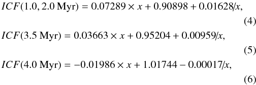
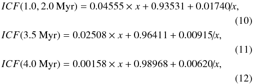
which are applicable for x ≳ 0.4, corresponding to the case for high-excitation H ii regions used for the ⁴He abundance determination. These fits are shown in Fig. 3 by red dashed, blue solid and green dotted lines for starburst ages of 1.0−2.0, 3.5, and 4.0 Myr, respectively. ICFs are lower for models with lower oxygen abundance 12 + log O/H = 7.3 and harder ionising radiation. They are higher for the highest metallicity models with 12 + log O/H = 8.3, because the spectral energy distribution of the ionising radiation is softer. ICFs derived from Eqs. (4)−(15), which we use below, are close to those used by e.g. Izotov et al. (2007). We found that ICF values are not sensitive to the assumption on the density distribution. Ionisation correction factors ICF(He) for all CLOUDY models (colour symbols in Fig. 3) are reproduced by the same fits for the homogeneous and inhomogeneous models.

Fig. 3 Ionisation correction factors ICF(He) vs. excitation parameter x = O2 +/O from the CLOUDY models with various oxygen abundances 12+log O/H and starburst ages. Red dashed, blue solid, and green dotted lines correspond to the starburst ages of 1.0−2.0, 3.5, 4.0 Myr, respectively. Symbols are CLOUDY-modelled data.

5. Non-recombination excitation of hydrogen

All element abundances in H ii regions are commonly derived relative to that of hydrogen. In particular, the ⁴He abundance is derived from the ratio of the recombination He i line intensity and the recombination intensity of the hydrogen Hβ emission line. Additionally, the observed Balmer decrement in real H ii regions is used for dust-reddening corrections. Therefore, prior to the reddening correction and abundance determination, hydrogen line intensities should be corrected for collisional and fluorescent excitation, which cause them to deviate from the recombination values. Much work has been done in previous studies to take these effects into account (see discussion and references in Izotov et al. 2007; Izotov & Thuan 2010).

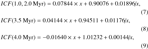
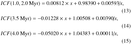
CLOUDY outputs allow one to obtain the fraction of non-recombination contribution (C + F)/I to intensities of hydrogen lines, where C and F are collisional and fluorescent contribution to the intensity, and I is the intensity. In particular, this contribution for the Hβ emission line is defined as a ratio [I(Hβ) – case B(Hβ)]/I(Hβ), where I(Hβ) is the Hβ intensity calculated with “all processes included” and case B(Hβ) is the case B recombination value. Similar expressions can be applied for other hydrogen lines. We used our grid of CLOUDY models to fit (C + F)/I for the four strongest Balmer hydrogen Hα, Hβ, Hγ, and Hδ emission lines as follows:

1. for the ages of 1.0 Myr and 2.0 Myr $\begin{array}{ccc}\frac{\mathit{C}\mathrm{+}\mathit{F}}{\mathit{I}}\mathrm{\left(}\mathrm{H}\mathit{\alpha }\mathrm{\right)}& \mathrm{=}& \mathrm{-}\mathrm{48.3963}\mathrm{+}\mathrm{19.0348}\mathit{A}\mathrm{\left(}\mathrm{O}\mathrm{\right)}\mathrm{-}\mathrm{2.4792}\mathit{A}\mathrm{(}\mathrm{O}{\mathrm{)}}^{\mathrm{2}}\\ & & \\ \frac{\mathit{C}\mathrm{+}\mathit{F}}{\mathit{I}}\mathrm{\left(}\mathrm{H}\mathit{\beta }\mathrm{\right)}& \mathrm{=}& \mathrm{-}\mathrm{28.3279}\mathrm{+}\mathrm{11.1685}\mathit{A}\mathrm{\left(}\mathrm{O}\mathrm{\right)}\mathrm{-}\mathrm{1.4571}\mathit{A}\mathrm{(}\mathrm{O}{\mathrm{)}}^{\mathrm{2}}\\ & & \\ \frac{\mathit{C}\mathrm{+}\mathit{F}}{\mathit{I}}\mathrm{\left(}\mathrm{H}\mathit{\gamma }\mathrm{\right)}& \mathrm{=}& \mathrm{-}\mathrm{24.3327}\mathrm{+}\mathrm{9.6403}\mathit{A}\mathrm{\left(}\mathrm{O}\mathrm{\right)}\mathrm{-}\mathrm{1.2631}\mathit{A}\mathrm{(}\mathrm{O}{\mathrm{)}}^{\mathrm{2}}\\ & & \\ \frac{\mathit{C}\mathrm{+}\mathit{F}}{\mathit{I}}\mathrm{\left(}\mathrm{H}\mathit{\delta }\mathrm{\right)}& \mathrm{=}& \mathrm{-}\mathrm{8.6082}\mathrm{+}\mathrm{3.5564}\mathit{A}\mathrm{\left(}\mathrm{O}\mathrm{\right)}\mathrm{-}\mathrm{0.4814}\mathit{A}\mathrm{(}\mathrm{O}{\mathrm{)}}^{\mathrm{2}}\\ & & \end{array}$

2. for the age of 3.5 Myr $\begin{array}{ccc}\frac{\mathit{C}\mathrm{+}\mathit{F}}{\mathit{I}}\mathrm{\left(}\mathrm{H}\mathit{\alpha }\mathrm{\right)}& \mathrm{=}& \mathrm{-}\mathrm{14.0001}\mathrm{+}\mathrm{5.7342}\mathit{A}\mathrm{\left(}\mathrm{O}\mathrm{\right)}\mathrm{-}\mathrm{0.7696}\mathit{A}\mathrm{(}\mathrm{O}{\mathrm{)}}^{\mathrm{2}}\\ & & \\ \frac{\mathit{C}\mathrm{+}\mathit{F}}{\mathit{I}}\mathrm{\left(}\mathrm{H}\mathit{\beta }\mathrm{\right)}& \mathrm{=}& \mathrm{-}\mathrm{7.6283}\mathrm{+}\mathrm{3.1765}\mathit{A}\mathrm{\left(}\mathrm{O}\mathrm{\right)}\mathrm{-}\mathrm{0.4315}\mathit{A}\mathrm{(}\mathrm{O}{\mathrm{)}}^{\mathrm{2}}\\ & & \\ \frac{\mathit{C}\mathrm{+}\mathit{F}}{\mathit{I}}\mathrm{\left(}\mathrm{H}\mathit{\gamma }\mathrm{\right)}& \mathrm{=}& \mathrm{3.2205}\mathrm{-}\mathrm{1.0250}\mathit{A}\mathrm{\left(}\mathrm{O}\mathrm{\right)}\mathrm{+}\mathrm{0.1099}\mathit{A}\mathrm{(}\mathrm{O}{\mathrm{)}}^{\mathrm{2}}\\ & & \\ \frac{\mathit{C}\mathrm{+}\mathit{F}}{\mathit{I}}\mathrm{\left(}\mathrm{H}\mathit{\delta }\mathrm{\right)}& \mathrm{=}& \mathrm{20.6912}\mathrm{-}\mathrm{7.7845}\mathit{A}\mathrm{\left(}\mathrm{O}\mathrm{\right)}\mathrm{+}\mathrm{0.9793}\mathit{A}\mathrm{(}\mathrm{O}{\mathrm{)}}^{\mathrm{2}}\\ & & \end{array}$

3. for the age of 4.0 Myr $\begin{array}{ccc}\frac{\mathit{C}\mathrm{+}\mathit{F}}{\mathit{I}}\mathrm{\left(}\mathrm{H}\mathit{\alpha }\mathrm{\right)}& \mathrm{=}& \mathrm{22.4758}\mathrm{-}\mathrm{8.4465}\mathit{A}\mathrm{\left(}\mathrm{O}\mathrm{\right)}\mathrm{+}\mathrm{1.0630}\mathit{A}\mathrm{(}\mathrm{O}{\mathrm{)}}^{\mathrm{2}}\\ & & \\ \frac{\mathit{C}\mathrm{+}\mathit{F}}{\mathit{I}}\mathrm{\left(}\mathrm{H}\mathit{\beta }\mathrm{\right)}& \mathrm{=}& \mathrm{21.3317}\mathrm{-}\mathrm{8.0875}\mathit{A}\mathrm{\left(}\mathrm{O}\mathrm{\right)}\mathrm{+}\mathrm{1.0252}\mathit{A}\mathrm{(}\mathrm{O}{\mathrm{)}}^{\mathrm{2}}\\ & & \\ \frac{\mathit{C}\mathrm{+}\mathit{F}}{\mathit{I}}\mathrm{\left(}\mathrm{H}\mathit{\gamma }\mathrm{\right)}& \mathrm{=}& \mathrm{33.8930}\mathrm{-}\mathrm{12.9456}\mathit{A}\mathrm{\left(}\mathrm{O}\mathrm{\right)}\mathrm{+}\mathrm{1.6505}\mathit{A}\mathrm{(}\mathrm{O}{\mathrm{)}}^{\mathrm{2}}\\ & & \\ \frac{\mathit{C}\mathrm{+}\mathit{F}}{\mathit{I}}\mathrm{\left(}\mathrm{H}\mathit{\delta }\mathrm{\right)}& \mathrm{=}& \mathrm{50.5361}\mathrm{-}\mathrm{19.3833}\mathit{A}\mathrm{\left(}\mathrm{O}\mathrm{\right)}\mathrm{+}\mathrm{2.4787}\mathit{A}\mathrm{(}\mathrm{O}{\mathrm{)}}^{\mathrm{2}}\\ & & \end{array}$where A(O) = 12 + log O/H.

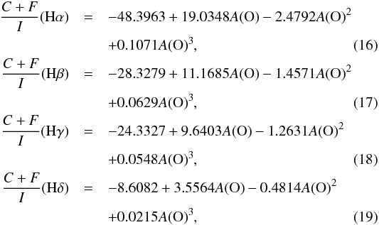
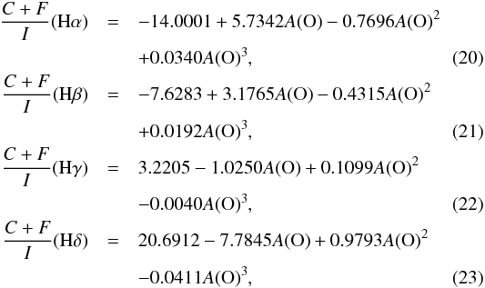
These fits are shown in Fig. 4 by red dashed, blue solid, and green dotted lines for models with starburst ages of 2.0, 3.5, and 4.0 Myr, respectively. It is seen from the figure that the non-recombination contribution in low-metallicity H ii regions can be as high as 9% and 6% for the Hα and other hydrogen lines, respectively. Neglecting this effect would result in appreciable underestimation of the ⁴He/H abundance ratio. Recently, Luridiana (2009) considered collisional excitation of hydrogen lines based on calculations with an earlier version of the CLOUDY code and probably with earlier set of the atomic data for hydrogen. She found that collisional contribution could be as high as 5% for the Hα emission line, or about twice as low as the non-recombination contribution in Fig. 4. In the following, we do not specify the collisional contribution and use the CLOUDY output values that include all processes that cause the hydrogen line intensities to deviate from the recombination values. In particular, fluorescent excitation may play a role, as was suggested by Luridiana et al. (2009). To derive the helium abundance we used the non-recombination contribution to the hydrogen line intensities obtained in the present paper.

Fig. 4 Non-recombination contribution of Balmer hydrogen line intensities as a function of the oxygen abundance. The red dashed, blue solid, and green dotted lines show fits for starburst ages of 2.0, 3.5, and 4.0 Myr, respectively. The dependences for starburst age of 1.0 Myr are identical to those for 2.0 Myr. Symbols are CLOUDY-modelled data.

6. Comparing the CLOUDY input and empirically derived values of the ⁴He abundance

Now we examine how well our empirical method described in Izotov & Thuan (2004) and Izotov et al. (2007) for determining the ⁴He abundance recovers the input ⁴He abundance in CLOUDY models. For this we first updated our empirical code so that its atomic ingredients were compatible with those used in CLOUDY: we incorporated the He i emissivities from Porter et al. (2013), the new data on the non-recombination excitation of hydrogen emission lines, and the new values of the ionisation correction factors for He obtained in the previous sections. Then we applied our updated empirical code to our 566 CLOUDY models, treating the CLOUDY output line intensities as if they were observed ones.

We used hydrogen line intensities calculated with CLOUDY, which include the non-recombination contribution. Furthermore, we used CLOUDY case B He i line intensities enhanced only by collisions. The latter was done because of the problems with CLOUDY He i line intensities for “all processes included” that we discussed in Sect. 3.2. Therefore, the fluorescent excitation of He i emission lines in the empirical method was set to zero when comparing with CLOUDY He i case B emission-line intensities. However, we note that in real H ii regions discussed below fluorescent excitation is taken into account to correct the observed intensities of He i emission lines. The CLOUDY forbidden line intensities of heavy elements were used to derive the electron temperature and heavy element abundances.

Then, we derived the ⁴He⁺ abundance ${\mathit{y}}_{\mathit{i}}^{\mathrm{+}}\mathrm{=}{\hspace{0.17em}}^{\mathrm{4}}{\mathrm{He}}_{\mathit{i}}^{\mathrm{+}}$/H⁺ from a number of strongest He i emission lines.

The weighted mean of the ${\mathit{y}}_{\mathit{i}}^{\mathrm{+}}$, ${\mathit{y}}_{\mathrm{wm}}^{\mathrm{+}}$, is defined by ${\mathit{y}}_{\mathrm{wm}}^{\mathrm{+}}\mathrm{=}\frac{{\sum }_{\mathit{i}}^{\mathit{n}}{\mathit{y}}_{\mathit{i}}^{\mathrm{+}}\mathit{/}{\mathit{\sigma }}^{\mathrm{2}}\mathrm{\left(}{\mathit{y}}_{\mathit{i}}^{\mathrm{+}}\mathrm{\right)}}{{\sum }_{\mathit{i}}^{\mathit{n}}\mathrm{1}\mathit{/}{\mathit{\sigma }}^{\mathrm{2}}\mathrm{\left(}{\mathit{y}}_{\mathit{i}}^{\mathrm{+}}\mathrm{\right)}}\mathit{,}$(28)where ${\mathit{y}}_{\mathit{i}}^{\mathrm{+}}$ is the ⁴He⁺ abundance derived from the intensity of the He i emission line labelled i, and $\mathit{\sigma }\mathrm{\left(}{\mathit{y}}_{\mathit{i}}^{\mathrm{+}}\mathrm{\right)}$ is the statistical error of ${\mathit{y}}_{\mathit{i}}^{\mathrm{+}}$.

We applied the Monte Carlo procedure described in Izotov & Thuan (2004) and Izotov et al. (2007), randomly varying the electron temperature T_e(He⁺) and the electron number density N_e(He⁺) within a specified range, to minimise the quantity ${\mathit{\chi }}^{\mathrm{2}}\mathrm{=}\sum _{\mathit{i}}^{\mathit{n}}\frac{\mathrm{(}{\mathit{y}}_{\mathit{i}}^{\mathrm{+}}\mathrm{-}{\mathit{y}}_{\mathrm{wm}}^{\mathrm{+}}{\mathrm{)}}^{\mathrm{2}}}{{\mathit{\sigma }}^{\mathrm{2}}\mathrm{\left(}{\mathit{y}}_{\mathit{i}}^{\mathrm{+}}\mathrm{\right)}}\mathrm{·}$(29)The resulting ${\mathit{y}}_{\mathrm{wm}}^{\mathrm{+}}$ is the value representing the empirically derived ⁴He⁺ abundance in each model.

In our comparison analysis we used ${\mathit{y}}_{\mathit{i}}^{\mathrm{+}}$ successively with equal weights and with weights proportional to the He i emission line intensity. The latter case is appropriate to the observational data because the intensities of weaker emission lines are more uncertain and therefore should be considered with lower weights.

Additionally, in cases with the nebular He ii λ4686 emission line, we added the abundance of doubly ionised helium y^2 + ≡ He²⁺/H⁺ to y⁺. Although the He²⁺ zone is hotter than the He⁺ zone, we adopted T_e(He²⁺) = T_e(He⁺). The last assumption has only a minor effect on the y value, because y²⁺ is small (≤0.5% of y⁺) in CLOUDY models.

The total ⁴He abundance y is obtained from the expression y = ICF(He) × (y⁺ + y^2 +) and is converted to the ⁴He mass fraction using equation $\mathit{Y}\mathrm{=}\frac{\mathrm{4}\mathit{y}\mathrm{(}\mathrm{1}\mathrm{-}\mathit{Z}\mathrm{)}}{\mathrm{1}\mathrm{+}\mathrm{4}\mathit{y}}\mathit{,}$(30)where Z = B × O/H is the heavy-element mass fraction. The coefficient B depends on O/Z, where O is the oxygen mass fraction. Maeder (1992) derived O/Z = 0.66 and 0.41 for Z = 0.001 and 0.02, respectively. The latter value is close to the most recent one in the Sun (0.43 using the abundances from Asplund et al. 2009). Adopting the Maeder (1992) values, we obtain B = 18.2 and 27.7 for Z = 0.001 and 0.02, respectively. In our calculations for every H ii region we used a value of B that linearly scales with A(O) (= 12 + log O/H) as follows: $\mathit{B}\mathrm{=}\mathrm{8.64}\mathit{A}\mathrm{\left(}\mathrm{O}\mathrm{\right)}\mathrm{-}\mathrm{47.44.}$(31)For comparison, Pagel et al. (1992) and Izotov et al. (2007), for example, used constant B of 20 and 18.2, respectively. We note, however, that neglecting the B – A(O) dependence would result in tiny uncertainties in Y, not exceeding 0.1% in the whole range of A(O) considered in this paper.

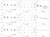Fig. 5 Distribution with the oxygen abundance of the empirically derived weighted mean Ya) and Neb) values calculated with the Porter et al. (2013) He i emissivities. Nine He i λ3889, λ4026, λ4388, λ4471, λ4922, λ5876, λ6678, λ7065, and λ10830 emission lines are used for χ2 minimisation and determination of Y. In the lower parts of the panels showing Y as a function of O/H we indicate the mean of all Y values derived from the models, together with the dispersion. Top: the electron temperature Te(He+) is randomly varied in the range $\mathrm{(}\mathrm{0.95}\mathrm{-}\mathrm{1.05}\mathrm{)}\mathrm{\times }\begin{array}{c}{}_{\mathrm{􏽥}}\\ {\mathit{T}}_{\mathrm{e}}\end{array}$(He+) where $\begin{array}{c}{\mathrm{􏽥}}_{}\\ {\mathit{T}}_{\mathrm{e}}\end{array}$(He+) is defined by Eq. (32), and the best derived values of Te(He+) for every model are shown in c). The solid line in a) shows the input CLOUDY Y value of 0.254, the dotted lines are 1% deviations, and ⟨ Y ⟩ is the average value of Ys shown by filled circles. Middle: the same as in the top panel, but Te(He+) = $\begin{array}{c}{\mathrm{􏽥}}_{}\\ {\mathit{T}}_{\mathrm{e}}\end{array}$(He+). Bottom: the same as in the top panel, but Te(He+) = Te(O iii).

In Fig. 5 we show the empirically derived oxygen abundances 12+log O/H, ⁴He mass fractions Y and the electron temperatures T_e(He⁺) from the CLOUDY-predicted emission-line intensities for all 566 models and the electron number densities N_e for 363 models with spatially constant number density. Here we adopted the Porter et al. (2013) He i emissivities defined by Eqs. (2) and (3) with coefficients from Tables 2 and 3. We used the nine strongest He i λ3889, λ4026, λ4388, λ4471, λ4922, λ5876, λ6678, λ7065, and λ10830 emission lines both for χ² minimisation and determination of the weighted mean Y. Equal weights for different lines were adopted. We varied N_e(He⁺) in our Monte Carlo simulations in the range 10−2 × 10³ cm^-3. The electron temperature T_e(O iii) was derived in our empirical routine from the [O iii]λ4363/(λ4959+λ5007) emission line intensity ratio prior to determining Y and is very close to the volume-emissivity-averaged value of the electron temperature in the O²⁺ zone calculated with CLOUDY grid models for the whole range of metallicities. For variations of the electron temperature T_e(He⁺) we adopted three cases:

1. the electron temperature T_e(He⁺) was randomly varied in the range (0.95−1.05) of the temperature derived from the relation between volume-averaged temperatures in our CLOUDY models, which can be fitted by the expression $\begin{array}{c}\mathrm{􏽥}\\ {\mathit{T}}_{\mathrm{e}}\end{array}\mathrm{\left(}{\mathrm{He}}^{\mathrm{+}}\mathrm{\right)}\mathrm{=}\mathrm{2.51}\mathrm{\times }{\mathrm{10}}^{-6}{\mathit{T}}_{\mathrm{e}}\mathrm{(}\mathrm{O}{iii}\mathrm{)}\mathrm{+}\mathrm{0.8756}\mathrm{+}\mathrm{1152}\mathit{/}{\mathit{T}}_{\mathrm{e}}\mathrm{(}\mathrm{O}{iii}\mathrm{)}\mathit{.}$(32)This relation predicts $\begin{array}{c}{\mathrm{􏽥}}_{}\\ {\mathit{T}}_{\mathrm{e}}\end{array}$(He⁺) <T_e(O iii) for hotter H ii regions and $\begin{array}{c}{\mathrm{􏽥}}_{}\\ {\mathit{T}}_{\mathrm{e}}\end{array}$(He⁺) >T_e(O iii) for cooler H ii regions;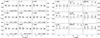

   Fig. 6 Left: distribution with the oxygen abundance of the empirical Y values calculated from the case B intensities for individual He i emission lines. The best values of Ys in every model are derived by varying Te(He+) in the range $\mathrm{(}\mathrm{0.95}\mathrm{-}\mathrm{1.05}\mathrm{)}\mathrm{\times }\begin{array}{c}{}_{\mathrm{􏽥}}\\ {\mathit{T}}_{\mathrm{e}}\end{array}$(He+). The definition of solid and dotted lines, and ⟨ Y ⟩ is the same as in Fig. 5. The mean value of Y is indicated at the bottom of each plot. Right: the same as in the left panel, but empirical Y values are calculated from the intensities for individual He i emission lines with all processes included.

2. T_e(He⁺) = $\begin{array}{c}{\mathrm{􏽥}}_{}\\ {\mathit{T}}_{\mathrm{e}}\end{array}$(He⁺);

3. T_e(He⁺) = T_e(O iii).

The results of our tests for the above three choices of T_e(He⁺) variations and randomly varying N_e(He⁺) are shown in Figs. 5a−5c, 5d−5e, and 5g−5i, respectively. In panels a, d, and g we indicate the mean of all Y values derived from the models, together with the dispersion. It is seen that empirically derived oxygen abundances 12 + log O/H (dots) agree well with the input CLOUDY values of 7.3, 7.6, 8.0, and 8.3 and deviate from them by not more than ~0.03 dex for 12 + log O/H = 7.3−8.0 and by ~0.06 dex for 12 + log O/H = 8.3. It is also seen from Figs. 5a, 5d, and 5g that the empirically derived ⁴He mass fractions Y (dots) agree well with the input CLOUDY value (solid line) and deviate from it by not more than at most 0.5% in most cases and only occasionally by up to 1.5%. The dispersion of the empirically derived Ys is slightly lower when the electron temperature T_e(He⁺) is varied in the range $\mathrm{(}\mathrm{0.95}\mathrm{-}\mathrm{1.05}\mathrm{)}\mathrm{\times }\begin{array}{c}{}_{\mathrm{􏽥}}\\ {\mathit{T}}_{\mathrm{e}}\end{array}$(He⁺) (Fig. 5c). The input CLOUDY number densities of 10, 10², and 10³ cm^-3 in models with spatially constant N_e are also very well reproduced (Figs. 5b, 5e, and 5h). We also note that despite the broad adopted range of T_e(He⁺) variations of $\mathrm{(}\mathrm{0.95}\mathrm{-}\mathrm{1.05}\mathrm{)}\mathrm{\times }\begin{array}{c}{}_{\mathrm{􏽥}}\\ {\mathit{T}}_{\mathrm{e}}\end{array}$(He⁺) for the models in the top panel of Fig. 5, its best derived values behave in Fig. 5c similar to values calculated with CLOUDY (Fig. 5f), suggesting that empirically derived T_e(He⁺) is also reproduced quite well.

In Fig. 6 (left panel) we show the ⁴He mass fractions Y empirically derived from the case B intensities of individual He i emission lines. These Y values correspond to the same empirical models as those in Fig. 5. Again, the empirically derived Ys (dots) broadly agree with the input CLOUDY value (solid lines). The poorest agreement is for the He i λ5876 and λ6678 emission lines in models with 12 + log O/H = 7.3. But even in these cases the empirical Y values on average do not deviate from the CLOUDY input value by more than 1%. We note that the most deviant points correspond to the models with Gaussian density distribution. These differences are mainly due to the larger uncertainties in the analytical fits of the He i emissivities at N_e ~ 10³ cm^-3 (dotted lines in Fig. 1). In any case, it is better to rely on several lines for an accurate derivation of Y, not only because of possible observational errors in line intensities, but also because of uncertainties in emissivities, their analytical fits, etc. For comparison, in Fig. 6 (right panel) are shown the ⁴He mass fractions Y empirically derived from the CLOUDY intensities of individual He i emission lines with all processes included. Note that in this case the correction for fluorescent excitation of He i emission lines is taken into account using the expressions given by Benjamin et al. (1999, 2002). The agreement between the CLOUDY input value of Y and empirically derived values is very poor, especially for He iλ5876 and λ6678 emission lines. This stems from the fact that, as noted in Sect. 3.2, the intensities of the lines calculated by CLOUDY with all processes included are not compatible with what we understand of the emission theory of these lines.

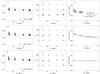Fig. 7 Same as in Fig. 5, but the five He i λ3889, λ4471, λ5876, λ6678, and λ7065 emission lines are used for χ2 minimisation and determination of Y.

The above analysis is based on empirical Y values, derived from the nine He i emission lines. However, in practice, a smaller number of He i emission lines is used for determining the ⁴He abundance. This is because He i emission lines λ4026, λ4388, λ4922 are several times weaker than the remaining He i emission lines and therefore their intensities are measured with lower accuracy. Furthermore, these emission lines are more subject to the uncertainties in correcting for underlying stellar He i absorption lines because of their low equivalent widths. Additionally, observations of the strongest near-infrared He i λ10830 emission line need facilities different from those used for the visible range. Therefore, this line is rarely observed in the low-metallicity emission-line galaxies. In particular, Izotov et al. (1994, 1997, 2007), and Izotov & Thuan (1998b, 2004, 2010), used only the five He i emission lines λ3889, λ4471, λ5876, λ6678, and λ7065 in the visible range for χ² minimisation in Eq. (29) (i.e. n = 5).

In Figs. 7a, d, and g we compare the empirically derived Ys for three choices of T_e(He⁺) variations with the input CLOUDY Y value in the case when the five He i emission lines λ3889, λ4471, λ5876, λ6678, and λ7065 are used for χ² minimisation in Eq. (29) and for determining the weighted mean value of Y. However, at variance with the case of the models with nine lines, we adopted weights for He i lines proportional to their intensity. This makes our comparison closer to real observations when stronger lines can be measured with better accuracy and therefore should be taken with heavier weights. Similarly to Fig. 5, we also compared the derived values of N_e and T_e(He⁺).

It is seen from Fig. 7c that the empirically derived electron temperature T_e(He⁺) has the same trend as the value calculated with CLOUDY (compare with Fig. 7f). Similarly, the empirically derived electron number density reproduces the CLOUDY input value fairly well (Fig. 7b). As a consequence, the empirical Ys are derived with accuracy similar to that in the case of nine lines. The accuracy of the Y determination is not as good when the electron temperature T_e(He⁺) is not varied, but is derived from Eq. (32) (middle panel of Fig. 7) or is equal to T_e(O iii) (bottom panel of Fig. 7). Ys in models with 12+log O/H = 7.3 and 7.6 are overestimated and show a high dispersion.

The above analysis indicates that five He i emission lines are quite enough to reproduce the input CLOUDY Y value with the desired accuracy; additional He i emission lines are needed if one wishes to reduce the dispersion of Ys at low oxygen abundances and to reduce trends seen in Figs. 7a, d, and g. Furthermore, we note that the most problematic emission line in the He abundance determination is the He i λ3889 line. This is because this line is blended with the hydrogen H8 λ3889 emission line and its intensity is subject to uncertainties of the subtraction of hydrogen emission and correction for underlying absorption not only of He i line, but also of H8 line. Therefore, the use of more He i emission lines would reduce the effect of these uncertainties. The most promising line for that is the strongest line, He i λ10830. This line is subject to a large extent to collisional excitation and therefore its intensity is sensitive to the electron number density N_e and electron temperature, and consequently, including it would better constrain both T_e and N_e.

In Fig. 8a, d, and g we show the empirical Ys derived by minimising χ² with the use of the six He i λ3889, λ4471, λ5876, λ6678, λ7065, and λ10830 emission lines. All these lines were used to determine the weighted mean Y with weights proportional to their intensities. The empirical Y values very well reproduce the input CLOUDY value, similar to the case of nine emission lines. The electron number density N_e is also reproduced very well (Figs. 8b, e, and h). The empirically derived T_e(He⁺) (Fig. 8c) follows the trend with T_e(O iii), similarly to that in the case of nine He i emission lines (Fig. 5c). Summarising, we conclude that our empirical technique satisfactorily reproduces the input CLOUDY Y values and can be used for the ⁴He abundance determination in real H ii regions.

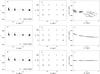Fig. 8 Same as in Fig. 5 but six He i λ3889, λ4471, λ5876, λ6678, λ7065, and λ10830 emission lines are used for the χ2 minimisation and the determination of Y.

7. Determining the ⁴He abundance in real H II regions

7.1. Method for determining the ⁴He abundance in real H II regions

While testing our empirical method on CLOUDY models calculated with the most recent v13.01 code, we took into account the new set of He i emissivities by Porter et al. (2013), the collisional excitation of He i emission lines, the non-recombination contribution to hydrogen emission-line intensities, and the correction for the ionisation structure of the H ii region.

To apply our empirical method to real H ii regions several other effects should be taken into account. First, the Balmer decrement corrected for the non-recombination contribution was used to simultaneously determine the dust extinction and equivalent widths of underlying stellar hydrogen absorption lines, as described for example by Izotov et al. (1994), and to correct line intensities for both effects. Second, since the spectra of the extragalactic H ii regions include both the ionised gas and the stellar emission, the underlying stellar He i absorption lines should be taken into account (see e.g. Izotov et al. 2007). Third, the He i emission lines should be corrected for fluorescent excitation that is parametrised by the optical depth τ(λ3889) of the He i λ3889 emission line. We used the correction factors for fluorescent excitation derived by Benjamin et al. (1999, 2002). The fluorescent excitation was not considered in test calculations because of the problems with the CLOUDY He i intensities when all processes are included (see Fig. 2 and discussion in Sect. 3).

Finally, the oxygen abundance should be corrected for its fraction locked in dust grains. Izotov et al. (2006) found that the Ne/O abundance ratio in low-metallicity emission-line galaxies increases with increasing oxygen abundance. They interpreted this trend by a larger fraction of oxygen locked in dust grains in galaxies with higher O/H. We used the relation of Izotov et al. (2006) between log Ne/O and 12 + log O/H to derive the fraction of oxygen confined in dust: 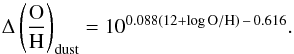$\mathrm{\Delta }{\left(\frac{\mathrm{O}}{\mathrm{H}}\right)}_{\mathrm{dust}}\mathrm{=}{\mathrm{10}}^{\mathrm{0.088}\mathrm{(}\mathrm{12}\mathrm{+}\log \mathrm{O}\mathit{/}\mathrm{H}\mathrm{)}\hspace{0.17em}\mathrm{-}\hspace{0.17em}\mathrm{0.616}}\mathit{.}$(33)The equivalent width of the He i λ4471 absorption line was chosen to be EW_abs(λ4471) = 0.4 Å, following González Delgado et al. (2005) and Izotov & Thuan (2010). The equivalent widths of the other absorption lines were fixed according to the ratios $\begin{array}{ccc}{\mathit{EW}}_{\mathrm{abs}}\mathrm{\left(}\mathit{\lambda }\mathrm{3889}\mathrm{\right)}\mathit{/}{\mathit{EW}}_{\mathrm{abs}}\mathrm{\left(}\mathit{\lambda }\mathrm{4471}\mathrm{\right)}& \mathrm{=}& \mathrm{1.0}\mathit{,}\\ {\mathit{EW}}_{\mathrm{abs}}\mathrm{\left(}\mathit{\lambda }\mathrm{5876}\mathrm{\right)}\mathit{/}{\mathit{EW}}_{\mathrm{abs}}\mathrm{\left(}\mathit{\lambda }\mathrm{4471}\mathrm{\right)}& \mathrm{=}& \mathrm{0.8}\mathit{,}\\ {\mathit{EW}}_{\mathrm{abs}}\mathrm{\left(}\mathit{\lambda }\mathrm{6678}\mathrm{\right)}\mathit{/}{\mathit{EW}}_{\mathrm{abs}}\mathrm{\left(}\mathit{\lambda }\mathrm{4471}\mathrm{\right)}& \mathrm{=}& \mathrm{0.4}\mathit{,}\\ {\mathit{EW}}_{\mathrm{abs}}\mathrm{\left(}\mathit{\lambda }\mathrm{7065}\mathrm{\right)}\mathit{/}{\mathit{EW}}_{\mathrm{abs}}\mathrm{\left(}\mathit{\lambda }\mathrm{4471}\mathrm{\right)}& \mathrm{=}& \end{array}$(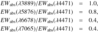34)The EW_abs(λ5876)/EW_abs(λ4471) and EW_abs(λ6678)/ EW_abs(λ4471) ratios were set equal to the values predicted for these ratios by a Starburst99 (Leitherer et al. 1999) instantaneous burst model with an age of 3−4 Myr and a heavy-element mass fraction Z = 0.001−0.008. These values are significantly higher than the corresponding ratios of 0.3 and 0.1 adopted by Izotov et al. (2007). We note that the value chosen for the EW_abs(λ5876)/ EW_abs(λ4471) ratio is also consistent with the one given by González Delgado et al. (2005). Since the output high-resolution spectra in Starburst99 are calculated only for wavelengths <7000 Å, we do not have a prediction for the EW_abs(λ7065)/EW_abs(λ4471) ratio. We set it to be equal to 0.4, the value of the EW_abs(λ6678)/ EW_abs(λ4471) ratio. As for He iλ3889, this line is blended with the hydrogen H8 λ3889 line. Therefore, EW_abs(He i λ3889) cannot be estimated from the Starburst99 models. We assumed the value shown in Eq. (34).

Finally, the age t_burst of a starburst should be derived. This is because ionisation correction factors ICF(He) and the non-recombination contribution to hydrogen lines both depend on the starburst age (see Sects. 4 and 5). As a first approximation, we used the relation between t_burst and EW(Hβ) from the Starburst99 instantaneous burst models with a heavy-element mass fraction Z = 0.004 (Leitherer et al. 1999). We fitted this relation by the expression 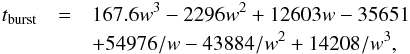$\begin{array}{ccc}{\mathit{t}}_{\mathrm{burst}}& \mathrm{=}& \mathrm{167.6}{\mathit{w}}^{\mathrm{3}}\mathrm{-}\mathrm{2296}{\mathit{w}}^{\mathrm{2}}\mathrm{+}\mathrm{12603}\mathit{w}\mathrm{-}\mathrm{35651}\\ & & \end{array}$(35)where t_burst is in Myr, w = log EW(Hβ) and EW(Hβ) is in Å. Eq. (35) does not take into account the contribution of old stellar populations in the underlying galaxy. The effect of an underlying galaxy is discussed in Sect. 8. Since the relations for Z = 0.001, Z = 0.004, and Z = 0.008 are similar at EW(Hβ) ≳ 100 Å, corresponding to t_burst ≲ 4 Myr, we adopted Eq. (35) for the entire range of oxygen abundances in our sample galaxies. We also adopted t_burst = 1 Myr and 4 Myr, when the derived starburst age was <1 Myr or >4 Myr. For t_burst in the range of 1−4 Myr we used the linear interpolation to derive ICF(He) (Eqs. (4)−(15)) and the non-recombination contribution to the intensities of hydrogen lines Hα, Hβ, Hγ, and Hδ (Eqs. (16)−(27)).

One caveat with the ionisation correction factors that we obtained from CLOUDY models is that they all have negligible y^2 +. However, in real H ii regions, the He iiλ4686 line is often measured but not explained (see Stasińska & Izotov 2003), and may give y^2 + as large as 3% that of y⁺. In particular, the He iiλ4686 line is measured in ~58% of spectra from our sample with an average intensity of ~1% that of Hβ, corresponding to ~1% of He in He²⁺ form. It tends to be stronger in H ii regions with lower metallicity. Thuan & Izotov (2005) and Izotov et al. (2012) proposed that a small fraction (a few percent) of ionising radiation could be produced by shocks. This radiation is harder than the stellar one and is responsible for He ii λ4686 emission, but only weakly influences the He i and H line intensities. However, we cannot quantify contribution of shocks using CLOUDY, and to estimate how ICF(He) changes when the small fraction of ionising radiation from shocks is present.

On the other hand, we can add some small fraction of harder non-thermal AGN-like ionising radiation to obtain the intensity of He ii λ4686 emission line of ~1%−3% that of the Hβ emission line. For this we assumed that the number of ionising photons due to the harder radiation is 5%−10% of the stellar number of ionising photons Q(H). Modelling with CLOUDY shows that the difference between ICF(He)’s with and without harder radiation is very small, not exceeding 0.2%.

7.2. Sample of low-metallicity emission-line galaxies

We determined Y_p and dY/d(O/H) for a large sample of low-metallicity emission-line galaxies, consisting of three subsamples. Most of our galaxies were compact. The spectra of these galaxies are obtained within apertures that are similar to or larger than the angular sizes. Therefore, these spectra are characteristics of the integrated galaxy properties averaged over their volume, not along the line of sight, and the above test analysis can be applied since it was made for volume-averaged characteristics.

The HeBCD subsample is composed of 93 different observations of 86 H ii regions in 77 galaxies. The majority of these galaxies are low-metallicity BCD galaxies. This sample is the same as the one described in Izotov & Thuan (2004, 2010).

The VLT subsample (Guseva et al. 2011) is composed of 75 VLT spectra of low-metallicity H ii regions selected from the ESO data archive.

The third subsample is composed of spectra of low-metallicity H ii regions selected from the SDSS DR7. The SDSS (York et al. 2000) offers a gigantic data base of galaxies with well-defined selection criteria and observed in a homogeneous way. In addition, the spectral resolution is much better than that of most previous data bases on emission-line galaxies including all the spectra in the HeBCD sample. First, we extracted ~15 000 spectra with strong emission lines from the whole data base of ~800 000 galaxy spectra. We measured the emission line intensities and determined the element abundances for the SDSS subsample following the same procedures as for the HeBCD and VLT subsamples. Then, for the ⁴He abundance determination, we selected 1442 spectra (SDSS subsample) in which the intensity of the temperature-sensitive emission line [O iii] λ4363 was measured with accuracy better than ~25%, allowing a reliable abundance determination. Part of the SDSS subsample was discussed for instance by Izotov et al. (2006, 2011a). In total, our sample consists of 1610 spectra, which we used to determine Y_p.

7.3. Linear regressions for determining the primordial ⁴He abundance

As in previous work (see Izotov et al. 2007; Izotov & Thuan 2010,and references therein), we determined the primordial ⁴He mass fraction Y_p by fitting the data points in the Y – O/H plane with a linear regression line of the form (Peimbert & Torres-Peimbert 1974, 1976; Pagel et al. 1992) 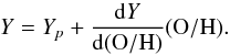$\mathit{Y}\mathrm{=}{\mathit{Y}}_{\mathit{p}}\mathrm{+}\frac{\mathrm{d}\mathit{Y}}{\mathrm{d}\mathrm{\left(}\mathrm{O}\mathit{/}\mathrm{H}\mathrm{\right)}}\mathrm{\left(}\mathrm{O}\mathit{/}\mathrm{H}\mathrm{\right)}\mathit{.}$(36)Assuming a linear dependence of Y on O/H appears to be reasonable because there are no evident non-linear trends in the distributions of the data points in the Y vs. O/H diagram (e.g., Izotov & Thuan 2004). The linear regression (Eq. (36)) implies that the initial mass function (IMF) averaged stellar yields for different elements do not depend on metallicity. It has been suggested in the past (e.g., Bond et al. 1983) that, at low metallicities, the IMF may be top-heavy, that is, that there are relatively more massive stars than lower mass stars than at high metallicities. If this is the case, the IMF-averaged yields would be significantly different for low-metallicity stars than those for more metal-enriched stars, resulting in a non-linear relationship between Y and O/H (Salvaterra & Ferrara 2003). However, until now, no persuasive evidence has been presented for a metallicity dependence of the IMF. Furthermore, the properties of extremely metal-deficient stars remain poorly known, excluding quantitative estimates of possible non-linear effects in the Y−O/H relation. Therefore, we continue to use the linear regression (Eq. (36)) to fit the data in the following analysis. However, for the sake of comparison we also consider non-linear fits.

To derive the parameters of the linear regressions, we used the maximum-likelihood method (Press et al. 1992), which takes into account the errors in Y and O/H for each object.

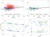Fig. 9 a)Y – O/H for the sample of 1610 H ii regions. The five He i emission lines λ3889, λ4471, λ5876, λ6678, and λ7065 are used for the χ2 minimisation and the determination of Y. Large blue and green filled circles are for the HeBCD and VLT samples, small red filled circles are SDSS galaxies. We chose to let Te(He+) vary freely in the range 0.95−1.05 of the $\begin{array}{c}{\mathrm{􏽥}}_{}\\ {\mathit{T}}_{\mathrm{e}}\end{array}$(He+) value. The continuous line represents the linear regression (whose equation is given at the bottom of the panel). b) Same as a), but only H ii regions with EW(Hβ) ≥ 100 Å are shown, with the excitation parameter x = O2+/O ≥ 0.7 and with 1σ error in Y ≤ 3%. The dotted line is the quadratic maximum-likelihood fit to the data. c) Distribution of the best derived values Te(He+)/Te(O iii) versus Te(O iii) for the case shown in b). d) Distribution of the best derived values Ne(He+) versus Ne(S ii) for the case shown in b).

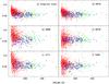Fig. 10 Distribution of helium mass fraction Y with Hβ equivalent width EW(Hβ) for the entire sample of 1610 H ii regions. Y values are the same as in Fig. 9a.

8. Primordial ⁴He mass fraction Y_p

We considered linear regressions Y – O/H for the entire HeBCD+VLT+SDSS sample, adopting that the electron temperature T_e(He⁺) is randomly varied in the range (0.95−1.05)$\begin{array}{c}{\mathrm{􏽥}}_{}\\ {\mathit{T}}_{\mathrm{e}}\end{array}$(He⁺) to minimise χ², where $\begin{array}{c}{\mathrm{􏽥}}_{}\\ {\mathit{T}}_{\mathrm{e}}\end{array}$(He⁺) is defined by Eq. (32). This regression is shown in Fig. 9a.

The most notable feature in the figure is that the SDSS H ii regions are offset relative to the HeBCD and VLT H ii regions. This suggests that HeBCD+VLT and SDSS H ii samples have different properties. First, the SDSS spectra are in general of lower quality, therefore the line intensities have much higher statistical errors. Second, SDSS galaxies have on average higher oxygen abundances. The temperature-sensitive [O iii] λ4363 emission line is weaker in their spectra and the electron temperature is derived with larger uncertainties. To study the sources of differences we show in Fig. 10 the dependences of the weighted mean ⁴He mass fraction Y and Ys derived from individual lines on the equivalent width EW(Hβ). It is clearly seen that the SDSS galaxies have on average lower EW(Hβ) and consequently lower EWs of He i emission lines. Therefore, the corrections for underlying stellar absorption in these objects are on average higher than those in HeBCD and VLT H ii regions, implying larger uncertainties caused by this effect.

We note the broad spread of Ys derived from the weakest He i λ4471, 6678, and 7065 emission lines in the SDSS spectra, implying that they have a lower quality than HeBCD and VLT spectra. As for the strongest λ3889 and λ5876 lines, the spread of Ys derived from the SDSS spectra is similar to that derived from the HeBCD and VLT spectra. However, the spread of Ys derived from the λ3889 emission line is much broader than that derived from the λ5876 emission line. Furthermore, it is much broader than that derived from faintest He i lines in the HeBCD and VLT samples. This line is blended with the hydrogen H8 line and therefore the determination of its intensity is more uncertain. This also implies that including an additional strong He i λ10830 emission line and its use instead of the He i λ3889 line is highly important to improve the determination of the He abundance.

The clear offset of the SDSS galaxies to higher Y values is seen in Fig. 10, with the possible exception for the λ6678 line. One of the likely reasons for this offset is that the SDSS spectra are obtained with a lower signal-to-noise ratio (S/N). Measurements with low S/Ns tend to be dominated by objects whose true value, for instance, the flux of the [O iii] λ4363 emission line, is slightly lower than the cutoff, and the uncertainties push them above the threshold (Malmquist-type bias). This effect is stronger for H ii regions with low EW(Hβ) where [O iii] λ4363 emission line in general is weaker, and it would potentially overestimate the electron temperature and He abundance. It can be decreased by selecting only spectra with highest S/N, for example, by selecting spectra whose He abundance is derived with an accuracy of better than 3%.

A similar offset of the SDSS H ii regions is seen in Fig. 11, where we show the dependence of the weighted mean Y on the excitation parameter x. The SDSS H ii regions are on average of lower excitation.

Summarising, we conclude that the ⁴He mass fractions Y in spectra of H ii regions with low EW(Hβ), low x and low S/N may be derived incorrectly. Therefore, in Fig. 9b we show the linear regression only for 182 high-excitation H ii regions with EW(Hβ) ≥ 100 Å, x ≥ 0.7 and with the 1σ error in Y value not exceeding 3%. There is no offset between H ii regions from different subsamples. We may further decrease the sample for instance by selecting objects with EW(Hβ) > 200 Å or/and selecting objects with σ(Y)/Y < 1%. However, in this case, the sample may become small and the Y_p value and the slope dY/d(O/H) derived from the maximum-likelihood regressions may not be very certain. We prefer to use a sample as large as possible.

The best derived values of the electron temperature T_e(He⁺) (Fig. 9c) are distributed within the entire range of the Monte Carlo variations, concentrating at the upper and lower values of 1.05$\begin{array}{c}{\mathrm{􏽥}}_{}\\ {\mathit{T}}_{\mathrm{e}}\end{array}$(He⁺) and 0.95$\begin{array}{c}{\mathrm{􏽥}}_{}\\ {\mathit{T}}_{\mathrm{e}}\end{array}$(He⁺), respectively, and do not follow the relation Eq. (32) between T_e(He⁺) and T_e(O iii) obtained from our CLOUDY models. This is somewhat surprising, and we do not have a good explanation for it. Note, however, that the reason cannot be the “temperature fluctuations” first studied by Peimbert (1967) and advocated by Peimbert et al. (2007), since in that case T_e(He⁺) is expected to be systematically lower than T_e(O iii). Furthermore, uncertainties of the He i line intensities may play a role. The best derived electron number density N_e(He⁺) does not correlate with the number density N_e(S ii) obtained from the [S ii] λ6717/λ6731 emission-line ratio (Fig. 9d). Of course, one does not expect this to be the case if the region of He i emission is not spatially coextensive with the region of [S ii] emission. However, for young and bright H ii regions one instead expects the inner zones to be denser than the outer ones, and this is not what Fig. 9d shows. A good test, but requiring very high S/N data, would be to compare N_e(He⁺) with the density derived from the [Cl iii] doublet.

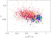Fig. 11 Distribution of helium mass fraction Y with the excitation parameter x = O2+/O for the entire sample of 1610 H ii regions. Y values are the same as in Fig. 9a.

Because we used a large sample of H ii regions, the statistical errors in the Y_p determination are small (e.g., Fig. 9b). On the other hand, other uncertainties can be significantly higher. These are uncertainties in the He i emissivities and their analytical fits (~1%, Fig. 1)¹, the uncertainties in ICF(He) (~0.25%, Fig. 3), and correction for the non-recombination contribution to hydrogen-line intensities (~0.5%, Fig. 4).

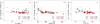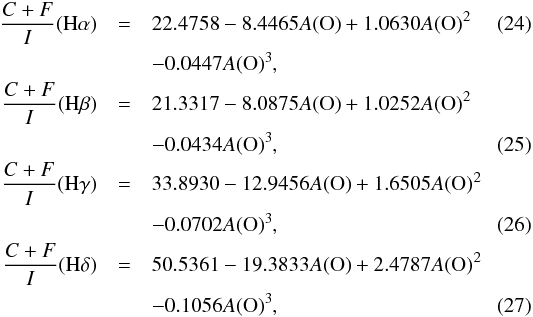
Fig. 12 a) Dependence of ΔICF(He)= ICF(EW(Hβ)) – ICF(SED) on the oxygen abundance 12 + log O/H for 64 SDSS galaxies with EW(Hβ) ≥ 100 Å, with the excitation parameter x = O2 +/O ≥ 0.7 and with 1σ error in Y ≤ 3% (dots) and for 32 SDSS galaxies with EW(Hβ) ≥ 150 Å, with the excitation parameter x = O2 +/O ≥ 0.8 and with 1σ error in Y ≤ 3% (encircled dots). Here ICF(EW(Hβ)) is the ionisation correction factor derived for a starburst age estimated from EW(Hβ), while ICF(SED) is the ionisation correction factor for the starburst age, which is derived from the spectral energy distribution (SED) fitting. Horizontal solid and dashed lines are average values of ΔICF(He) for dots and encircled dots, respectively. b) The dependence of ΔICF(He) = ICF(EW(Hβ)) – ICF(SED) on the Hβ equivalent width EW(Hβ). Symbols and lines have the same meaning as in a). c) The dependence of ΔICF(He) = ICF(EW(Hβ)) – ICF(SED) on the excitation parameter x. Symbols and lines have the same meaning as in a).

One of the systematic uncertainties is caused by the presence of the underlying galaxy. Owing to this effect, the EW(Hβ) is decreased and the starburst age is overestimated, resulting in overestimated ICF(He) and Y. To estimate the effect of the underlying galaxy we show in Fig. 12 the dependence of the difference ΔICF(He) = ICF(EW(Hβ)) – ICF(SED) for SDSS galaxies from Fig. 9b on the oxygen abundance 12 + log O/H, Hβ equivalent width EW(Hβ), and excitation parameter x = O^2 +/O. Here, ICF(EW(Hβ)) is the ionisation correction factor derived for a starburst age estimated from EW(Hβ), while ICF(SED) is the ionisation correction factor for the starburst age, which was derived from the spectral energy distribution (SED) fitting. To fit the SED we followed the technique described by Izotov et al. (2011a). Briefly, it takes into account the emission of the young and old stellar populations as well as the ionised gas emission.

It is evident that ICF(EW(Hβ)) >ICF(SED) because the starburst age derived from the SED fitting is always younger than that derived from EW(Hβ). The effect of the underlying galaxy on ICF in galaxies with EW(Hβ) ≥ 100 Å, x ≥ 0.7 and ΔY/Y ≤ 3% (dots in Fig. 12) is small, ~0.4% on average (horizontal solid line). We note that there is no clear trend of ΔICF(He) on 12 + log O/H (Fig. 12a). On the other hand, there is an increase of ΔICF(He) with decreasing EW(Hβ) (Fig. 12b) and x (Fig. 12c), suggesting that the effect of an underlying galaxy is higher for lower-excitation H ii regions that are older.

However, if only H ii regions with EW(Hβ) ≥ 150 Å and x ≥ 0.8 are considered (encircled dots in Fig. 12), no dependence on EW(Hβ) and x is detected with a very low average ΔICF(He)= 0.25% (horizontal dashed line). Thus, from the above discussion of Y_p systematic errors (1% due to the uncertainties in the He i emissivities and their analytical fits, 0.25% due to the uncertainties in ICF fits, 0.5% due to the uncertainties in correction for the non-recombination contribution to hydrogen-line intensities and 0.25% due to the contribution of the underlying galaxy), we adopted the value $\sqrt{{\mathrm{1}}^{\mathrm{2}}\mathrm{+}{\mathrm{0.5}}^{\mathrm{2}}\mathrm{+}{\mathrm{0.25}}^{\mathrm{2}}\mathrm{+}{\mathrm{0.25}}^{\mathrm{2}}}$% = 1.17% or σ(Y_p) = 0.003.

As a final sample for determining Y_p we adopted the sample of 111 H ii regions satisfying conditions EW(Hβ) ≥ 150 Å, x ≥ 0.8 and ΔY/Y ≤ 3%. The linear regression for this sample is shown in Fig. 13 with the primordial value Y_p = 0.2542.

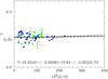Fig. 13 Y – O/H for the sample of 111 H ii regions with EW(Hβ) ≥ 150 Å, with the excitation parameter x = O2+/O ≥ 0.8 and with 1σ error in Y ≤ 3%. The five He i emission lines λ3889, λ4471, λ5876, λ6678, and λ7065 are used for χ2 minimisation and determination of Y. Large blue and green filled circles are for HeBCD and VLT samples, respectively, small red filled circles are SDSS galaxies. We chose to let Te(He+) vary freely in the range 0.95−1.05 of the $\begin{array}{c}{\mathrm{􏽥}}_{}\\ {\mathit{T}}_{\mathrm{e}}\end{array}$(He+) value. The continuous line represents the linear regression (whose equation is given at the bottom of the panel) and the dashed lines are 1σ alternatives of the linear regression. The dotted line is the quadratic maximum-likelihood fit to the data.

Since the statistical error of Y_p (±0.0006) is much lower than the systematic error, we finally adopted ${\mathit{Y}}_{\mathrm{p}}\mathrm{=}\mathrm{0.254}\mathrm{\pm }\mathrm{0.003.}$(37)This new Y_p agrees with the Y_ps derived by Izotov & Thuan (2010) and Aver et al. (2012). However, this agreement is in fact accidental because different He i emissivities and corrections for non-recombination excitation of hydrogen lines were used in different studies.

The linear dependence Y – O/H in Fig. 13 is not steep. The weighted mean of all 111 data points in the figure is Y = 0.255 with χ² = 6.13 per degree of freedom. These values are slightly higher than Y_p = 0.254 and χ² = 6.12 per degree of freedom returned by the linear maximum-likelihood technique, implying only weak linear dependence. Additionally, we calculated the quadratic maximum-likelihood regression (dotted line in Fig. 13) and obtained a primordial value of 0.255 with χ² = 5.39 per degree of freedom. We preferred to use the Y_p value derived from the linear regression over the weighted mean value because chemical evolution models predict a general increase of the He abundance with O/H. The same chemical evolution argument does not favour the quadratic regression because the He abundance at low oxygen abundances is lower with increasing O/H.

9. Cosmological implications

We have derived the primordial ⁴He mass fraction Y_p = 0.254 ± 0.003 (Fig. 13), which is higher than the SBBN value of 0.2477 ± 0.0001 inferred from the analysis of the temperature fluctuations of the microwave background radiation (Ade et al. 2013), indicating deviations from the standard rate of Hubble expansion in the early Universe. These deviations can be caused by an extra contribution to the total energy density (for example by additional species of neutrinos), which can be parameterised by an equivalent number of neutrino species N_eff.

To derive N_eff we used the statistical χ² technique with the code described by Fiorentini et al. (1998) and Lisi et al. (1999) to analyse the constraints that the measured ⁴He and D abundances put on η and N_eff. The joint fits of η and N_eff are shown in Fig. 14. With the two freedoms of degree (η₁₀ and N_eff), the deviations at the 68.3% confidence level (CL) corresponding to ${\mathit{\chi }}^{\mathrm{2}}\mathrm{-}{\mathit{\chi }}_{\min }^{\mathrm{2}}\mathrm{=}\mathrm{2.30}$, at the 95.4% CL corresponding to ${\mathit{\chi }}^{\mathrm{2}}\mathrm{-}{\mathit{\chi }}_{\min }^{\mathrm{2}}\mathrm{=}\mathrm{6.17}$, and at the 99.0% CL corresponding to ${\mathit{\chi }}^{\mathrm{2}}\mathrm{-}{\mathit{\chi }}_{\min }^{\mathrm{2}}\mathrm{=}\mathrm{9.21}$ are shown (from the inside out) by solid lines.

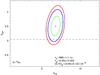Fig. 14 Joint fits to the baryon-to-photon number ratio, η10=1010η, and the equivalent number of light neutrino species Neff, using a χ2 analysis with the code developed by Fiorentini et al. (1998) and Lisi et al. (1999). The value of the primordial 4He abundance has been set to Yp = 0.254 (Fig. 13) and that of (D/H)p is taken from Pettini & Cooke (2012). The neutron lifetime of τn = 880.1 ± 1.1s from Beringer et al. (2012) has been adopted. The filled circle corresponds to ${\mathit{\chi }}^{\mathrm{2}}\mathrm{=}{\mathit{\chi }}_{\min }^{\mathrm{2}}\mathrm{=}\mathrm{0}$. Solid lines from the inside out correspond to confidence levels of 68.3% (${\mathit{\chi }}^{\mathrm{2}}\mathrm{-}{\mathit{\chi }}_{\min }^{\mathrm{2}}\mathrm{=}\mathrm{2.30}$), 95.4% (${\mathit{\chi }}^{\mathrm{2}}\mathrm{-}{\mathit{\chi }}_{\min }^{\mathrm{2}}\mathrm{=}\mathrm{6.17}$) and 99.0% (${\mathit{\chi }}^{\mathrm{2}}\mathrm{-}{\mathit{\chi }}_{\min }^{\mathrm{2}}\mathrm{=}\mathrm{9.21}$), respectively. The SBBN value Neff = 3.046 is shown with a dashed line.

We adopted the most recently published value for neutron lifetimes τ_n = 880.1 ± 1.1 s (Beringer et al. 2012). With Y_p = 0.254 ± 0.003, (D/H)_p = (2.60 ± 0.12) × 10^-5 (Pettini & Cooke 2012), the minimum ${\mathit{\chi }}_{\min }^{\mathrm{2}}\mathrm{=}\mathrm{0}$ is obtained for η₁₀ = 6.42, corresponding to Ω_bh² = 0.0234 ± 0.0019 and N_eff = 3.51 ± 0.35 (68% CL) (Fig. 14). This value of N_eff at the 68% CL is higher than the SBBN value N_ν = 3.

We note that the primordial helium abundance sets a tight constraint on the effective number of neutrino species. These constraints are similar to or are tighter than those derived using the CMB and galaxy clustering power spectra. For example, using these two sets of data, Komatsu et al. (2011) derived ${\mathit{N}}_{\mathrm{eff}}\mathrm{=}\mathrm{4.3}{\mathrm{4}}_{-0.88}^{\mathrm{+}\mathrm{0.86}}$ at the 68% confidence level. On the other hand, Keisler et al. (2011) analysed joint WMAP7 data and South Pole Telescope (SPT) data, both on the microwave background temperature fluctuations, and derived N_eff = 3.85 ± 0.62 (68% CL). Adding low-redshift measurements of the Hubble constant H₀ using the Hubble Space Telescope and the baryon acoustic oscillations (BAO) using SDSS and 2dFGRS, Keisler et al. (2011) obtained N_eff = 3.86 ± 0.42 (68% CL).

On the other hand, Ade et al. (2013) using the data of the Planck mission derived N_eff = 3.30 ± 0.27 (68% CL). Thus, there is a general agreement between N_eff obtained in this paper and by other researchers with other methods. However, uncertainties are too high to make definite conclusions about the deviations of the BBN from the standard model. Tighter constraints can be obtained by including the additional He i λ10830 emission line in the consideration, which requires new observations. This work is in progress.

Our baryon mass density Ω_bh² = 0.0234 ± 0.0019 (68% CL) (Fig. 14) agrees with the values of 0.0222 ± 0.0004 (Keisler et al. 2011) and 0.0221 ± 0.0003 (Ade et al. 2013) from fluctuation studies of the CMB radiation. Arbey (2012) developed the most recent code AlterBBN for calculating BBN abundances of the elements in alternative cosmologies. Adopting a neutron lifetime of τ_n = 880.1 s (Beringer et al. 2012), our derived N_eff = 3.51 and η₁₀ = 6.42, it returns the predicted primordial abundances Y_p = 0.253 and (D/H)_p = 2.53 × 10^-5, which agree well with the values obtained from observations.

10. Conclusions

We have rederived the pregalactic helium abundance, improving on several aspects with respect to our previous estimates. First, we used the updated He i emissivities published by Porter et al. (2013), tested our overall procedure on a grid of CLOUDY models built with the most recent version of the code, v13.01 (Ferland et al. 2013), using the same atomic data. Most importantly, we used the largest possible set of suitable observational data, which significantly enhance the set used by Izotov & Thuan (2010), thus reducing the statistical error in determining Y_p and allowing a more comprehensive analysis of systematic effects.

Before proceeding to determine Y in real objects, we produced analytical fits to the grid of He i emissivities published by Porter et al. (2013); then we tested and refined our procedure to derive the helium mass fraction in H ii regions using an appropriate grid of photoionisation models built with CLOUDY.

Finally, we applied our updated empirical code for the determination of the primordial ⁴He abundance from the largest sample of low-metallicity extragalactic H ii regions ever used (1610 spectra). It consists of three subsamples: a) the HeBCD subsample of low-metallicity and high-excitation H ii regions used for instance by Izotov et al. (2007) and Izotov & Thuan (2010) for the primordial ⁴He abundance determination (93 spectra), b) the VLT subsample of low-metallicity and high-excitation H ii regions collected by Guseva et al. (2011) and Izotov et al. (2009, 2011b) from the European Southern Observatory (ESO) archive (75 spectra), and c) the SDSS subsample of generally lower-excitation H ii regions (1442 spectra). Our main results are summarised below.

• 1.

  We fitted the new tabulated He i emissivi-ties by Porter et al. (2013).Our fits reproduced the tabulated emissivities of32 He i emission lines with an ac-curacy of better than 1% in a wide range of electron temperaturesT_e = 10   000−20   000 K and electron number densities N_e = 10−10³ cm^-3.

• 2.

  We obtained ionisation correction factors for He from CLOUDY-photoionised H ii region models and produced fits to them as a function of the starburst age and the excitation parameter x = O²⁺/O, where O and O²⁺ are the total oxygen abundance and the abundance of the doubly ionised oxygen, respectively. The new ionisation correction factors agree well with previously published ones, used for instance by Izotov et al. (2007) and Izotov & Thuan (2010).

• 3.

  We derived from CLOUDY models the non-recombination contribution to the strongest hydrogen Balmer emission line intensities, which includes both the collisional and fluorescent excitation. For that we compared the hydrogen line intensities calculated including all processes with their case B values. We found that the non-recombination contribution to the Hα and Hβ line intensities can be as high as ~9% and ~6%, respectively, in the hot lowest-metallicity H ii regions. We produced the fits of these contributions as a function of the oxygen abundance and starburst age.

• 4.

  We used the CLOUDY-predicted emission-line intensities to recover the physical conditions and chemical composition of the H ii region models using our updated empirical method. We found that our method reproduces the electron number density N_e(He⁺) and the emissivity-weighted electron temperature T_e(He⁺). Most importantly, the empirical method reproduces the CLOUDY input value of the ⁴He mass fraction with an accuracy of better than 1%, independently of the number of He i emission lines used for the χ² minimisation. This gives confidence in our method for determining the ⁴He abundance in real H ii regions.

• 5.

  We applied our updated empirical method for determining the ⁴He mass fraction Y to a large sample of 1610 low-metallicity extragalactic H ii regions. This is the largest sample used for such a study. We found a systematic offset between Ys derived for the HeBCD+VLT and SDSS subsamples, indicating problems in the Y determination in most of SDSS H ii regions. However, the offset is not present when only spectra with the highest S/N of the highest-excitation HeBCD+VLT+SDSS H ii regions are used. Using linear relation Y – O/H for 111 highest-excitation H ii regions we derived the primordial ⁴He mass fraction Y_p = 0.254 ± 0.003, which is higher than the standard big bang nucleosynthesis (SBBN) value of 0.2477 ± 0.0001 inferred from the temperature fluctuations of the microwave background radiation. This difference possibly indicates the existence of additional types of neutrino species.

• 6.

  Using the most recently derived primordial abundances of light elements D and ⁴He and the χ² technique, we found that the best agreement between abundances of these light elements is achieved in the BBN model with the baryon mass fraction Ω_bh² = 0.0234 ± 0.0019 (68% CL) and the effective number of the neutrino species N_eff = 3.51 ± 0.35 (68% CL). Both the Ω_bh² and N_eff values nicely agree with those inferred from the temperature fluctuations of the microwave background radiation.

Note added in proof. Ryan Porter (priv. comm.) pointed out that the difference we found between the case B He i intensities and the He i intensities calculated with all processes included (see Sect. 3.2) is due to our using an insufficient number of He i states (n = 6, the default value). Indeed, we find that the agreement between He i line intensities and case B intensities for triplet transitions, including the He i 5876 line, is better than 1% only when n is greater than 25. However, the calculation time is then increased by a factor of more than 20, which prevents the production of our grid of models in a reasonable computing time. Since our subsequent analysis is based on the case B intensities to which we add the other effects “by hand”, the results of our paper remain correct.

Online material

Acknowledgments

Y.I.I. is thankful to the Observatoire de Paris for financing a three-month stay during which part of this work was done. This paper makes extensive use of the photoionisation code CLOUDY, and we are grateful to its authors, in particular G. Ferland. Funding for the Sloan Digital Sky Survey (SDSS) and SDSS-II has been provided by the Alfred P. Sloan Foundation, the Participating Institutions, the National Science Foundation, the US Department of Energy, the National Aeronautics and Space Administration, the Japanese Monbukagakusho, the Max Planck Society, and the Higher Education Funding Council for England.

References

All Tables

All Figures

	Fig. 1 Comparison of calculated and fitted emissivities of the strongest He i emission lines for three values of the electron number densities Ne = 10, 102, and 103 cm-3. Collisional excitation is taken into account.
In the text

	Fig. 2 Ratio of the CLOUDY-calculated intensities with all processes included to CLOUDY case B intensities for several brightest He i emission lines as a function of the oxygen abundance for the models with low electron number density Ne = 10 cm-3. For clarity only models with log Q(H) = 53 are shown.
In the text

	Fig. 3 Ionisation correction factors ICF(He) vs. excitation parameter x = O2 +/O from the CLOUDY models with various oxygen abundances 12+log O/H and starburst ages. Red dashed, blue solid, and green dotted lines correspond to the starburst ages of 1.0−2.0, 3.5, 4.0 Myr, respectively. Symbols are CLOUDY-modelled data.
In the text

	Fig. 4 Non-recombination contribution of Balmer hydrogen line intensities as a function of the oxygen abundance. The red dashed, blue solid, and green dotted lines show fits for starburst ages of 2.0, 3.5, and 4.0 Myr, respectively. The dependences for starburst age of 1.0 Myr are identical to those for 2.0 Myr. Symbols are CLOUDY-modelled data.
In the text

Fig. 5 Distribution with the oxygen abundance of the empirically derived weighted mean Ya) and Neb) values calculated with the Porter et al. (2013) He i emissivities. Nine He i λ3889, λ4026, λ4388, λ4471, λ4922, λ5876, λ6678, λ7065, and λ10830 emission lines are used for χ2 minimisation and determination of Y. In the lower parts of the panels showing Y as a function of O/H we indicate the mean of all Y values derived from the models, together with the dispersion. Top: the electron temperature Te(He+) is randomly varied in the range $\mathrm{(}\mathrm{0.95}\mathrm{-}\mathrm{1.05}\mathrm{)}\mathrm{\times }\begin{array}{c}{}_{\mathrm{􏽥}}\\ {\mathit{T}}_{\mathrm{e}}\end{array}$(He+) where $\begin{array}{c}{\mathrm{􏽥}}_{}\\ {\mathit{T}}_{\mathrm{e}}\end{array}$(He+) is defined by Eq. (32), and the best derived values of Te(He+) for every model are shown in c). The solid line in a) shows the input CLOUDY Y value of 0.254, the dotted lines are 1% deviations, and ⟨ Y ⟩ is the average value of Ys shown by filled circles. Middle: the same as in the top panel, but Te(He+) = $\begin{array}{c}{\mathrm{􏽥}}_{}\\ {\mathit{T}}_{\mathrm{e}}\end{array}$(He+). Bottom: the same as in the top panel, but Te(He+) = Te(O iii).

In the text

Fig. 6 Left: distribution with the oxygen abundance of the empirical Y values calculated from the case B intensities for individual He i emission lines. The best values of Ys in every model are derived by varying Te(He+) in the range $\mathrm{(}\mathrm{0.95}\mathrm{-}\mathrm{1.05}\mathrm{)}\mathrm{\times }\begin{array}{c}{}_{\mathrm{􏽥}}\\ {\mathit{T}}_{\mathrm{e}}\end{array}$(He+). The definition of solid and dotted lines, and ⟨ Y ⟩ is the same as in Fig. 5. The mean value of Y is indicated at the bottom of each plot. Right: the same as in the left panel, but empirical Y values are calculated from the intensities for individual He i emission lines with all processes included.

In the text

	Fig. 7 Same as in Fig. 5, but the five He i λ3889, λ4471, λ5876, λ6678, and λ7065 emission lines are used for χ2 minimisation and determination of Y.
In the text

	Fig. 8 Same as in Fig. 5 but six He i λ3889, λ4471, λ5876, λ6678, λ7065, and λ10830 emission lines are used for the χ2 minimisation and the determination of Y.
In the text

Fig. 9 a)Y – O/H for the sample of 1610 H ii regions. The five He i emission lines λ3889, λ4471, λ5876, λ6678, and λ7065 are used for the χ2 minimisation and the determination of Y. Large blue and green filled circles are for the HeBCD and VLT samples, small red filled circles are SDSS galaxies. We chose to let Te(He+) vary freely in the range 0.95−1.05 of the $\begin{array}{c}{\mathrm{􏽥}}_{}\\ {\mathit{T}}_{\mathrm{e}}\end{array}$(He+) value. The continuous line represents the linear regression (whose equation is given at the bottom of the panel). b) Same as a), but only H ii regions with EW(Hβ) ≥ 100 Å are shown, with the excitation parameter x = O2+/O ≥ 0.7 and with 1σ error in Y ≤ 3%. The dotted line is the quadratic maximum-likelihood fit to the data. c) Distribution of the best derived values Te(He+)/Te(O iii) versus Te(O iii) for the case shown in b). d) Distribution of the best derived values Ne(He+) versus Ne(S ii) for the case shown in b).

In the text

	Fig. 10 Distribution of helium mass fraction Y with Hβ equivalent width EW(Hβ) for the entire sample of 1610 H ii regions. Y values are the same as in Fig. 9a.
In the text

	Fig. 11 Distribution of helium mass fraction Y with the excitation parameter x = O2+/O for the entire sample of 1610 H ii regions. Y values are the same as in Fig. 9a.
In the text

Fig. 12 a) Dependence of ΔICF(He)= ICF(EW(Hβ)) – ICF(SED) on the oxygen abundance 12 + log O/H for 64 SDSS galaxies with EW(Hβ) ≥ 100 Å, with the excitation parameter x = O2 +/O ≥ 0.7 and with 1σ error in Y ≤ 3% (dots) and for 32 SDSS galaxies with EW(Hβ) ≥ 150 Å, with the excitation parameter x = O2 +/O ≥ 0.8 and with 1σ error in Y ≤ 3% (encircled dots). Here ICF(EW(Hβ)) is the ionisation correction factor derived for a starburst age estimated from EW(Hβ), while ICF(SED) is the ionisation correction factor for the starburst age, which is derived from the spectral energy distribution (SED) fitting. Horizontal solid and dashed lines are average values of ΔICF(He) for dots and encircled dots, respectively. b) The dependence of ΔICF(He) = ICF(EW(Hβ)) – ICF(SED) on the Hβ equivalent width EW(Hβ). Symbols and lines have the same meaning as in a). c) The dependence of ΔICF(He) = ICF(EW(Hβ)) – ICF(SED) on the excitation parameter x. Symbols and lines have the same meaning as in a).

In the text

Fig. 13 Y – O/H for the sample of 111 H ii regions with EW(Hβ) ≥ 150 Å, with the excitation parameter x = O2+/O ≥ 0.8 and with 1σ error in Y ≤ 3%. The five He i emission lines λ3889, λ4471, λ5876, λ6678, and λ7065 are used for χ2 minimisation and determination of Y. Large blue and green filled circles are for HeBCD and VLT samples, respectively, small red filled circles are SDSS galaxies. We chose to let Te(He+) vary freely in the range 0.95−1.05 of the $\begin{array}{c}{\mathrm{􏽥}}_{}\\ {\mathit{T}}_{\mathrm{e}}\end{array}$(He+) value. The continuous line represents the linear regression (whose equation is given at the bottom of the panel) and the dashed lines are 1σ alternatives of the linear regression. The dotted line is the quadratic maximum-likelihood fit to the data.

In the text

Fig. 14 Joint fits to the baryon-to-photon number ratio, η10=1010η, and the equivalent number of light neutrino species Neff, using a χ2 analysis with the code developed by Fiorentini et al. (1998) and Lisi et al. (1999). The value of the primordial 4He abundance has been set to Yp = 0.254 (Fig. 13) and that of (D/H)p is taken from Pettini & Cooke (2012). The neutron lifetime of τn = 880.1 ± 1.1s from Beringer et al. (2012) has been adopted. The filled circle corresponds to ${\mathit{\chi }}^{\mathrm{2}}\mathrm{=}{\mathit{\chi }}_{\min }^{\mathrm{2}}\mathrm{=}\mathrm{0}$. Solid lines from the inside out correspond to confidence levels of 68.3% (${\mathit{\chi }}^{\mathrm{2}}\mathrm{-}{\mathit{\chi }}_{\min }^{\mathrm{2}}\mathrm{=}\mathrm{2.30}$), 95.4% (${\mathit{\chi }}^{\mathrm{2}}\mathrm{-}{\mathit{\chi }}_{\min }^{\mathrm{2}}\mathrm{=}\mathrm{6.17}$) and 99.0% (${\mathit{\chi }}^{\mathrm{2}}\mathrm{-}{\mathit{\chi }}_{\min }^{\mathrm{2}}\mathrm{=}\mathrm{9.21}$), respectively. The SBBN value Neff = 3.046 is shown with a dashed line.

In the text

References

- Arbey, A. 2012, Comp. Phys. Comm., 183, 1822 [Google Scholar]
- Asplund, M., Grevesse, N., & Sauval, A. J., & Scott, P. 2009, ARA&A, 47, 481 [NASA ADS] [CrossRef] [Google Scholar]
- Aver, E., Olive, K. A., & Skillman, E. D. 2010, J. Cosmol. Astropart. Phys., 05, 003A [Google Scholar]
- Aver, E., Olive, K. A., & Skillman, E. D. 2011, J. Cosmol. Astropart. Phys., 03, 043A [CrossRef] [Google Scholar]
- Aver, E., Olive, K. A., & Skillman, E. D. 2012, J. Cosmol. Astropart. Phys., 04, 004A [Google Scholar]
- Benjamin, R. A., Skillman, E. D., & Smits, D. P. 1999, ApJ, 514, 307 [NASA ADS] [CrossRef] [Google Scholar]
- Benjamin, R. A., Skillman, E. D., & Smits, D. P. 2002, ApJ, 569, 288 [NASA ADS] [CrossRef] [Google Scholar]
- Beringer, J., et al. (Particle Data Group) 2012, Phys. Rev. D, 86, 010001 [Google Scholar]
- Bond, J. R., Carr, B. J., & Arnett, W. D. 1983, Nature, 304, 514 [NASA ADS] [CrossRef] [Google Scholar]
- Ferland, G. J., Korista, K. T., Verner, D. A., et al. 1998, PASP, 110, 761 [Google Scholar]
- Ferland, G. J., Porter, R. L., van Hoof, P. A. M., et al. 2013, Rev. Mex. Astron. Astrofis., 49, 137 [Google Scholar]
- Fiorentini, G., Lisi, E., Sarkar, S., & Villante, F. L. 1998, Phys. Rev. D, 58, 063506 [NASA ADS] [CrossRef] [Google Scholar]
- González Delgado, R. M., Cerviño, M., Martins, L. P., Leitherer, C., & Hauschildt, P. H. 2005, MNRAS, 357, 945 [NASA ADS] [CrossRef] [Google Scholar]
- Guseva, N. G., Izotov, Y. I., Stasińska, G., et al. 2011, A&A, 529, A149 [NASA ADS] [CrossRef] [EDP Sciences] [Google Scholar]
- Hillier, D. J., & Miller, D. L. 1998, ApJ, 496, 407 [NASA ADS] [CrossRef] [Google Scholar]
- Iocco, F., Mangano, G., Miele, G., Pisanti, O., & Serpico, P. D. 2009, Phys. Rept., 472, 1 [Google Scholar]
- Izotov, Y. I., & Thuan, T. X. 1998, ApJ, 500, 188 [NASA ADS] [CrossRef] [Google Scholar]
- Izotov, Y. I., & Thuan, T. X. 2004, ApJ, 602, 200 [CrossRef] [Google Scholar]
- Izotov, Y. I., & Thuan, T. X. 2010, ApJ, 710, L67 [NASA ADS] [CrossRef] [EDP Sciences] [MathSciNet] [Google Scholar]
- Izotov, Y. I., Thuan, T. X., & Lipovetsky, V. A. 1994, ApJ, 435, 647 [NASA ADS] [CrossRef] [Google Scholar]
- Izotov, Y. I., Thuan, T. X., & Lipovetsky, V. A. 1997, ApJS, 108, 1 [NASA ADS] [CrossRef] [Google Scholar]
- Izotov, Y. I., Stasińska, G., Meynet, G., Guseva, N. G., & Thuan, T. X. 2006, A&A, 448, 955 [NASA ADS] [CrossRef] [EDP Sciences] [Google Scholar]
- Izotov, Y. I., Thuan, T. X., & Stasińska, G. 2007, ApJ, 662, 15 [NASA ADS] [CrossRef] [Google Scholar]
- Izotov, Y. I., Guseva, N. G., Fricke, K. J., & Papaderos, P. 2009, A&A, 503, 61 [NASA ADS] [CrossRef] [EDP Sciences] [Google Scholar]
- Izotov, Y. I., Guseva, N. G., & Thuan, T. X. 2011a, ApJ, 728, 161 [NASA ADS] [CrossRef] [Google Scholar]
- Izotov, Y. I., Guseva, N. G., Fricke, K. J., & Henkel, C. 2011b, A&A, 533, A25 [NASA ADS] [CrossRef] [EDP Sciences] [Google Scholar]
- Izotov, Y. I., Thuan, T. X., Privon, G. 2012, MNRAS, 427, 1229 [NASA ADS] [CrossRef] [Google Scholar]
- Keisler, R., Reichard C. L., Aird, K. A., et al. 2011, ApJ, 743, 28 [NASA ADS] [CrossRef] [Google Scholar]
- Kingdon, J., & Ferland, G. J. 1995, ApJ, 442, 714 [NASA ADS] [CrossRef] [Google Scholar]
- Komatsu, E., Smith, K. M. Dunkley, J., et al. 2011, ApJS, 192, 18 [NASA ADS] [CrossRef] [Google Scholar]
- Leitherer, C., Schaerer, D., Goldader, J. D., et al. 1999, ApJS, 123, 3 [NASA ADS] [CrossRef] [Google Scholar]
- Lisi, E., Sarkar, S., & Villante, F. L. 1999, Phys. Rev. D, 59, 123520 [NASA ADS] [CrossRef] [Google Scholar]
- Luridiana, V. 2009, Ap&SS, 324, 361 [NASA ADS] [CrossRef] [Google Scholar]
- Luridiana, V., Simón-Díaz, S., Cerviño, M., et al. 2009, ApJ, 691, 1712 [NASA ADS] [CrossRef] [Google Scholar]
- Maeder, A. 1992, A&A, 264, 105 [NASA ADS] [Google Scholar]
- Meynet, G., Maeder, A., Schaller, G., Schaerer, D., & Charbonnel, C. 1994, A&AS, 103, 97 [Google Scholar]
- Noterdaeme, P., López, S., Dumont, V., et al. 2012, A&A, 542, L33 [NASA ADS] [CrossRef] [EDP Sciences] [Google Scholar]
- Pagel, B. E. J., Simonson, E. A., Terlevich, R. J., & Edmunds, M. G. 1992, MNRAS, 255, 325 [NASA ADS] [CrossRef] [Google Scholar]
- Pauldrach, A. W. A., Hoffman, T. L., & Lennon, M. 2001, A&A, 375, 161 [NASA ADS] [CrossRef] [EDP Sciences] [Google Scholar]
- Peimbert, M. 1967, ApJ, 150, 825 [NASA ADS] [CrossRef] [Google Scholar]
- Peimbert, M., & Torres-Peimbert, S. 1974, ApJ, 193, 327 [NASA ADS] [CrossRef] [Google Scholar]
- Peimbert, M., & Torres-Peimbert, S. 1976, ApJ, 203, 581 [NASA ADS] [CrossRef] [Google Scholar]
- Peimbert, M., Luridiana, V., & Peimbert, A. 2007, ApJ, 666, 636 [NASA ADS] [CrossRef] [Google Scholar]
- Pettini, M., & Cooke, R. 2012, MNRAS, 425, 2477 [CrossRef] [Google Scholar]
- Planck Collaboration 2013, A&A, in press [arXiv:1303.5076] [Google Scholar]
- Porter, R. L., Ferland, G. J., & MacAdam, K. B. 2007, ApJ, 657, 327 [NASA ADS] [CrossRef] [Google Scholar]
- Porter, R. L., Ferland, G. J., MacAdam, K. B., & Storey, P. J. 2009, MNRAS, 393, L36 [NASA ADS] [Google Scholar]
- Porter, R. L., Ferland, G. J., Storey, P. J., & Detisch, M. J. 2012, MNRAS, 425, L28 [NASA ADS] [Google Scholar]
- Porter, R. L., Ferland, G. J., Storey, P. J., & Detisch, M. J. 2013, MNRAS, 433, L89 [NASA ADS] [CrossRef] [Google Scholar]
- Press, W. H., Teukolsky, S. A., Vetterling, W. T., & Flannery, B. P., 1992, Numerical Recipes in C, The Art of Scientific Computing, 2nd edn. (Cambrige: Cambrige University Press) [Google Scholar]
- Salvaterra, R., & Ferrara, A. 2003, MNRAS, 340, L17 [NASA ADS] [CrossRef] [Google Scholar]
- Stasińska, G., & Izotov, Y. I. 2003, A&A, 397, 71 [NASA ADS] [CrossRef] [EDP Sciences] [Google Scholar]
- Steigman, G. 2005, Phys. Scr., T121, 142 [Google Scholar]
- Steigman, G. 2006, Int. J. Mod. Phys. E, 15, 1 [Google Scholar]
- Steigman, G. 2012 [arXiv:1208.0032] [Google Scholar]
- Thuan, T. X., & Izotov, Y. I. 2005, ApJS, 161, 240 [NASA ADS] [CrossRef] [Google Scholar]
- York, D. G., Adelman, J., Anderson, J. E., Jr., et al. 2000, AJ, 120, 1579 [Google Scholar]
All Tables
Fit parameters for the relative collisional contributions, C/R, to the He i line emissivities.