| Issue |
A&A
Volume 557, September 2013
|
|
|---|---|---|
| Article Number | A92 | |
| Number of page(s) | 11 | |
| Section | Galactic structure, stellar clusters and populations | |
| DOI | https://doi.org/10.1051/0004-6361/201321559 | |
| Published online | 06 September 2013 | |
The asymmetric drift, the local standard of rest, and implications from RAVE data
1
Astronomisches Rechen-Institut, Zentrum für Astronomie der Universität
Heidelberg,
Mönchhofstr. 12–14,
69120
Heidelberg,
Germany
e-mail:
This email address is being protected from spambots. You need JavaScript enabled to view it.
2
Department of Aerospace Engineering Sciences, University of
Colorado at Boulder, 429
UCB, Boulder,
CO
80309,
USA
3
Institute of Astronomy, Kharkiv National University,
35 Sumska Str., 61022
Kharkiv,
Ukraine
4
Observatoire astronomique de Strasbourg, 11 rue de
l’Université, 67000
Strasbourg,
France
5
Sydney Institute for Astronomy, School of Physics A28, University
of Sydney, NSW
2006
Sydney,
Australia
6
Dept of Phys & Astro, Saint Marys Univ,
Halifax, B3H 3C3, Canada
7
Monash Centre for Astrophysics, 3800
Clayton,
Australia
8
Jeremiah Horrocks Institute, UCLan, Preston, PR1
2HE, UK
9
NAF Osservatorio Astronomico di Padova,
36012
Asiago,
Italy
10
Department of Physics & Astronomy, University of
Victoria, Victoria,
BC, V8P 5C2, Canada
11
Department of Physics & Astronomy, Macquarie
University, NSW,
2109
Sydney,
Australia
12
Macquarie Research Centre for Astronomy, Astrophysics and
Astrophotonics, 2109
Sydney,
Australia
13
Australian Astronomical Observatory, PO Box 296, Epping, NSW
2121
Sydney,
Australia
14
Mullard Space Science Laboratory, University College
London, Holmbury St
Mary, Dorking,
RH5 6NT,
UK
15
Department of Physics and Astronomy, Padova
University, Vicolo
dell’Osservatorio 2, 35122
Padova,
Italy
16
Leibniz-Institut für Astrophysik Potsdam (AIP),
An der Sternwarte 16,
14482
Potsdam,
Germany
17
Faculty of Mathematics and Physics, University of
Ljubljana, Jadranska
19, 1000
Ljubljana,
Slovenia
18
Center of Excellence SPACE-SI, Askerceva cesta 12,
1000
Ljubljana,
Slovenia
Received:
25
March
2013
Accepted:
27
June
2013
Abstract
Context. The determination of the local standard of rest (LSR), which corresponds to the measurement of the peculiar motion of the Sun based on the derivation of the asymmetric drift of stellar populations, is still a matter of debate. The classical value of the tangential peculiar motion of the Sun with respect to the LSR was challenged in recent years, claiming a significantly larger value.
Aims. We present an improved Jeans analysis, which allows a better interpretation of the measured kinematics of stellar populations in the Milky Way disc. We show that the Radial Velocity Experiment (RAVE) sample of dwarf stars is an excellent data set to derive tighter boundary conditions to chemodynamical evolution models of the extended solar neighbourhood.
Methods. We propose an improved version of the Strömberg relation with the radial scalelengths as the only unknown. We redetermine the asymmetric drift and the LSR for dwarf stars based on RAVE data. Additionally, we discuss the impact of adopting a different LSR value on the individual scalelengths of the subpopulations.
Results. Binning RAVE stars in metallicity reveals a bigger asymmetric drift (corresponding to a smaller radial scalelength) for more metal-rich populations. With the standard assumption of velocity-dispersion independent radial scalelengths in each metallicity bin, we redetermine the LSR. The new Strömberg equation yields a joint LSR value of V⊙ = 3.06 ± 0.68 km s-1, which is even smaller than the classical value based on Hipparcos data. The corresponding radial scalelength increases from 1.6 kpc for the metal-rich bin to 2.9 kpc for the metal-poor bin, with a trend of an even larger scalelength for young metal-poor stars. When adopting the recent Schönrich value of V⊙ = 12.24 km s-1 for the LSR, the new Strömberg equation yields much larger individual radial scalelengths of the RAVE subpopulations, which seem unphysical in part.
Conclusions. The new Strömberg equation allows a cleaner interpretation of the kinematic data of disc stars in terms of radial scalelengths. Lifting the LSR value by a few km s-1 compared to the classical value results in strongly increased radial scalelengths with a trend of smaller values for larger velocity dispersions.
Key words: Galaxy: kinematics and dynamics / solar neighborhood
© ESO, 2013
1. Introduction
In any dynamical model of the Milky Way, the rotation curve (which is the circular speed vc(R) as function of distance R to the Galactic centre) plays a fundamental role. In axisymmetric models the mean tangential speed vc of stellar subpopulations deviates from vc, which is quantified by the asymmetric drift Va. Converting observed kinematic data (with respect to the Sun) to a Galactic coordinate system requires additionally the knowledge of the peculiar motion of the Sun with respect to the local circular speed.
The asymmetric drift of a stellar population is defined as the difference between the
velocity of a hypothetical set of stars possessing perfectly circular orbits and the mean
rotation velocity of the population under consideration. The velocity of the former is
called the standard of rest. If the measurements are made at the solar Galactocentric
radius, it is the local standard of rest (LSR). The determination of the LSR corresponds to
measuring the peculiar motion
(U⊙,V⊙,W⊙)
of the Sun, where U⊙ is the velocity of the Sun in the direction
of the Galactic centre, V⊙ in the direction of the Galactic
rotation, and W⊙ in the vertical direction. While measuring
U⊙ and W⊙ is relatively
straightforward, V⊙ requires a sophisticated asymmetric drift
correction for its measurement, which is one goal of this paper. The asymmetric drift
 is the difference of
the local circular speed vc and the mean rotational speed
is the difference of
the local circular speed vc and the mean rotational speed
 of the stellar population. The asymmetric drift corresponds (traditionally with a minus sign
to yield positive values for Va) to the measured mean rotational
velocity of the stellar sample corrected by the reflex motion of the Sun.
of the stellar population. The asymmetric drift corresponds (traditionally with a minus sign
to yield positive values for Va) to the measured mean rotational
velocity of the stellar sample corrected by the reflex motion of the Sun.
The main problem is to disentangle the asymmetric drift Va of
each subpopulation and the peculiar motion of the Sun V⊙ using
measured mean tangential velocities  . For any stellar subpopulation
in dynamical equilibrium, the Jeans equation (Eq. (2)) provides a connection of the asymmetric drift, radial scalelengths, and
properties of the velocity dispersion ellipsoid in axisymmetric systems (Binney & Tremaine 2008). There are two principal
ways to determine both Va and V⊙
with the help of the Jeans equation. The direct path would be to measure for one tracer
population the radial gradient of the volume density ν and of the radial
velocity dispersion in the Galactic plane together with the inclination of the velocity
ellipsoid away from the Galactic plane additionally to the local velocity ellipsoid. This
approach is still very challenging due to observational biases in spatially extended stellar
samples (by extinction close to the midplane, distance-dependent selection biases etc.).
Therefore we need to stick to the classical approach to apply the Jeans equation to a set of
subpopulations and assume common properties or dependencies of the radial scalelengths and
the velocity ellipsoid.
. For any stellar subpopulation
in dynamical equilibrium, the Jeans equation (Eq. (2)) provides a connection of the asymmetric drift, radial scalelengths, and
properties of the velocity dispersion ellipsoid in axisymmetric systems (Binney & Tremaine 2008). There are two principal
ways to determine both Va and V⊙
with the help of the Jeans equation. The direct path would be to measure for one tracer
population the radial gradient of the volume density ν and of the radial
velocity dispersion in the Galactic plane together with the inclination of the velocity
ellipsoid away from the Galactic plane additionally to the local velocity ellipsoid. This
approach is still very challenging due to observational biases in spatially extended stellar
samples (by extinction close to the midplane, distance-dependent selection biases etc.).
Therefore we need to stick to the classical approach to apply the Jeans equation to a set of
subpopulations and assume common properties or dependencies of the radial scalelengths and
the velocity ellipsoid.
On top of this basic equilibrium model, non-axisymmetric perturbations like spiral arms may lead to a significant shift in the local mean velocities of tracer populations (see Siebert et al. 2011a, 2012, for the first direct measurement of a gradient in the mean radial velocity and the interpretation in terms of spiral arms). In the present paper we focus on the discussion of the Jeans equation in axisymmetric models.
In the classical approach the Jeans equation is applied to local stellar samples of different (mean) age, which show increasing velocity dispersion with increasing age due to the age-velocity dispersion relation. Up to the end of the last century, the general observation that the mean tangential velocity depends linearly on the squared velocity dispersion for stellar populations that are not too young allowed the measurement of V⊙ by extrapolation to zero velocity dispersion. The corresponding reformulation of the Jeans equation is the famous linear Strömberg equation (Eq. (4)). This method was also used by Dehnen & Binney (1998) for a volume-complete sample of Hipparcos stars to constrain the LSR. They found again that the asymmetric drift Va depends linearly on the squared (three-dimensional) velocity dispersion of a stellar population. A linear extrapolation to zero velocity dispersion led to the LSR. The velocity of the Sun in the direction of the Galactic rotation with respect to the LSR appeared to be V⊙ = 5.25 ± 0.62 km s-1. Aumer & Binney (2009) applied a similar approach to the new reduction of the Hipparcos catalogue and obtained the same value V⊙ = 5.25 ± 0.54 km s-1, but with a smaller error bar. The linear Strömberg relation (Binney & Tremaine 2008) adopted in this analysis relies on the crucial assumption that the structure (radial scalelengths and shape of the velocity dispersion ellipsoid) of the subpopulations with different velocity dispersions are similar.
In recent years it was argued, based on very different methods, that the value of
V⊙ should be increased significantly. Based on a sophisticated
dynamical model of the extended solar neighbourhood, Binney
(2010) argued that the V component of the Sun’s peculiar velocity
should be revised upwards to ≈11 km s-1. In McMillan & Binney (2010) it was shown that
V⊙ ≈ 11 km s-1 would be more appropriate based on the
space velocities of maser sources in star-forming regions (Reid et al. 2009). The chemodynamical model of the Milky-Way-like galaxy of Schönrich et al. (2010) shows a non-linear dependence
 . This implies different radial
scalelengths and/or different shapes of the velocity ellipsoid for different subpopulations.
Fitting the observed dependence by predictions of their model,
they got V⊙ = 12.24 ± 0.47 km s-1, which is also
significantly larger than the classical value. Most recently Bovy et al. (2012b) derived an even larger value of
V⊙ ≈ 24 km s-1 based on Apogee data and argued for an
additional non-axisymmetric motion of the locally observed LSR of 10 km s-1
compared to the real circular motion.
. This implies different radial
scalelengths and/or different shapes of the velocity ellipsoid for different subpopulations.
Fitting the observed dependence by predictions of their model,
they got V⊙ = 12.24 ± 0.47 km s-1, which is also
significantly larger than the classical value. Most recently Bovy et al. (2012b) derived an even larger value of
V⊙ ≈ 24 km s-1 based on Apogee data and argued for an
additional non-axisymmetric motion of the locally observed LSR of 10 km s-1
compared to the real circular motion.
In view of the inside-out growth of galactic discs (established by the observed radial colour and metallicity gradients), there is no a priori reason why stellar subpopulations with different velocity dispersion should have similar radial scalelengths independent of the significance of radial migration processes (Matteucci & Francois 1989; Chiappini & Matteuchi 2001; Wielen et al. 1996; Schoenrich & Binney 2009a,b; Scannapieco 2011; Minchev et al. 2013). Therefore it is worthwhile to step back and investigate the consequences of the Jeans equation in a more general context. The fact that the peculiar motion of the Sun (i.e. the definition of the LSR) is one and the same unique value entering the dynamics of all stellar subpopulations already shows that changing the observed value for V⊙ will have a wide range of consequences for our understanding of the structure and evolution of the Milky Way disc.
The goal of this paper is twofold. We discuss the Jeans equation in a more general context and derive a new version of the Strömberg equation that is useful for an improved method to analyse the interrelation of radial scalelengths, the asymmetric drift, and the LSR. We emphasize the impact of different choices of LSR. Secondly, we apply the new method to the large and homogeneous sample of dwarf stars provided by the latest internal data release (May 15th, 2012) of the RAVE (see Steinmetz et al. 2006; Zwitter et al. 2008; Siebert et al. 2011b, for the first, second, and third data release respectively) and complement it with other data sets. In Sect. 2 we describe the data analysis, Sect. 3 contains the Jeans analysis, in Sect. 4 our results are presented, and Sect. 5 concludes with a discussion.
2. Data analysis
For our analysis we use several different kinematically unbiased data sets. In all the cases, only stars with heliocentric distances r < 3 kpc and Galactocentric radii 7.5 kpc < R < 8.5 kpc and with distances to the mid-plane | z| < 500 pc are selected. A list of variables used in the paper are collected in Table 1.
Variables used in the paper.
Even though most stars in our samples are relatively local, we make all computations in Galactocentric cylindrical coordinates. That is why we need to fix the Galactocentre distance R0 and the circular speed v⊙ for our computations: they influence how velocities of distant stars are decomposed into radial and rotational components. We adopt R0 = 8 kpc, which is consistent with most observational data to date (Reid 1993; Gilessen et al. 2009). Assuming Sgr A* to reside at the centre of the Galaxy at rest and taking μl,A∗ = 6.37 ± 0.02 mas yr-1 for its proper motion in the Galactic plane (Reid & Brunthaler 2005), we find the rotation velocity of the Sun to be v⊙ = 241.6 km s-1 in a Galactocentric coordinate system. This velocity consists of the circular velocity in the solar neighbourhood vc (of the LSR) and the peculiar velocity of the Sun with respect to the LSR V⊙, so that v⊙ = vc + V⊙. For the radial and vertical components of the LSR, we assume U⊙ = 9.96 km s-1 and W⊙ = 7.07 km s-1 from Aumer & Binney (2009).
Any radial or vertical gradient of the mean velocity and velocity dispersions may influence
the determination of the corresponding values at the solar position. Linear trends cancel
out for symmetric samples with respect to the solar position, but spatially asymmetric
samples can result in shifts of mean velocity and velocity dispersions. Additionally,
spatial gradients of the mean velocities result in an overestimation of the velocity
dispersions due to the shifted mean values at the individual positions of the stars. For
example, for the tangential velocity dispersion
σφ we find  (1)Here
vφ is the tangential velocity of the stars,
(1)Here
vφ is the tangential velocity of the stars,
 the
sample mean,
the
sample mean,  is the
root mean square (rms) value of the difference of the mean tangential velocity at the
individual positions of the stars to the sample mean, and
δvφ is the rms of the
propagated individual measurement errors. In our analysis we do not take the described
effects into account but discuss the potential impact on our results.
is the
root mean square (rms) value of the difference of the mean tangential velocity at the
individual positions of the stars to the sample mean, and
δvφ is the rms of the
propagated individual measurement errors. In our analysis we do not take the described
effects into account but discuss the potential impact on our results.
Despite the RAVE sample being the biggest one, supplementing it with other samples provides an important consistency check as all samples have different selection criteria and biases, different sources of distance measurements, and are differently divided into subsamples with different kinematics.
2.1. RAVE data
For the upcoming fourth data release the stellar parameter pipeline to derive effective temperature, surface gravity, and metallicity was improved significantly. The latest internal data release is based on the new stellar parameter pipeline and contains 402 721 stars. Internally, there are two independent catalogues of distances available. The first is based on isochrone fitting in the colour-magnitude diagram (CMD; Zwitter et al. 2010), which contains 383 387 stars in the updated version. The second method is based on a Bayesian analysis of the stellar parameters (Burnett et al. 2011) and contains 201 670 stars. For these stars line of sight velocities vr, proper motions μ, temperatures Teff, surface gravities log g, and metallicities [M/H] are measured. The J and K colours are taken from the Two Micron All Sky Survey (2MASS; Skrutskie et al. 2006).
For our analysis we selected stars with absolute distance errors Δr/r ≤ 0.3, proper motion errors Δμ ≤ 10 mas yr-1, radial velocity errors Δvr ≤ 3 km s-1, Galactic latitudes | b| ≥ 20°. The CMD of the selected stars is shown in Fig. 1 with colour-coded log g. Furthermore, we selected only stars that meet the criterion 0.75 < K − 4(J − K) < 2.75 (see Fig. 1), primarily to exclude subgiants and giants. Finally, a total number N = 68 670 stars remain.
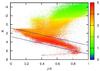 |
Fig. 1 CMD of the full RAVE sample based on Zwitter distances. Surface gravity log g is colour-coded and the lines show the selected dwarf stars. |
To obtain subsamples with different kinematics, the stars are binned according to their J − K colours. These subsamples show a clear systematic trend with colour in the mean tangential velocity ΔV and in the radial velocity dispersion σR (see Fig. 2). We find a larger velocity dispersion with decreasing metallicity, as expected. But in contrast to the general expectation, the corresponding asymmetric drift is decreasing with decreasing metallicity, meaning faster rotation of lower metallicity populations. This inverted trend is more pronounced in the bluer colour bins with a younger mean age of the subpopulations. A similar trend was already observed in the thin disc sample of G dwarfs from the Sloan Extension for Galactic Understanding and Exploration (SEGUE; Lee et al. 2011b; Liu & van de Ven 2012) and for the younger population in the Geneva-Copenhagen Survey (Loebman et al. 2011).
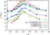 |
Fig. 2 Measured mean tangential velocity ΔV (full circles) and radial velocity dispersion σR (crosses) of the RAVE sample based on Zwitter distances as functions of J − K colour. |
We do not attempt to separate thin and thick disc stars, but due to the vertical limitation | z| ≤ 500 pc the thin disc is expected to dominate. Instead, we split the samples in the colour bins further into three metallicity bins, −0.5 < [M/H] < −0.2, −0.2 < [M/H] < 0, and 0 < [M/H] < 0.2. Even though the absolute calibration of the RAVE metallicity is not completely settled (Boeche et al. 2011), the metallicity [M/H] from the RAVE pipeline can be used as a relative indicator of the true metallicity. The subsample properties are collected in Table 2. The total number of stars in this colour and metallicity range is N = 63 978, with 44%, 47%, and 9% falling into the low, middle, and high metallicity bin respectively.
Properties of the RAVE sample.
From Table 2 we see that different bins probe slightly different volumes, with bluer bins (which correspond to brighter stars) extending farther both in radial and vertical directions. Due to the asymmetry of the RAVE sample, the mean radius R differs from R0 = 8 kpc and the mean height z differs from 0, with the difference also being larger for bluer bins. These small variations and offset have no significant impact on the derivation of the kinematic properties at the solar position. It is important to mention that the volume occupied by a subsample does not strongly depend on its metallicity and that the metal-poor stars are on average about 30% farther away from the Sun than the metal-rich stars only for the reddest bin.
To take full advantage of the stellar parameter estimation in RAVE, we measure the shape
of the velocity ellipsoid. In Fig. 3 the upper panel
shows the squared ratio of the velocity dispersions in the rotational and radial
directions,  . There is a
trend with velocity dispersion (which is discussed more in Sect. 5) but no significant differences for different metallicities. In the
epicyclic approximation, the ratio is connected to the local rotation curve by
. There is a
trend with velocity dispersion (which is discussed more in Sect. 5) but no significant differences for different metallicities. In the
epicyclic approximation, the ratio is connected to the local rotation curve by
 for standard values (Binney & Tremaine 2008), where
κ is the epicyclic frequency in the solar neighbourhood and Ω is the
orbital frequency. The observed deviations may be due to spiral structure of the Galactic
disc at the low-velocity-dispersion end and to the non-harmonic motion with respect to the
guiding centre of stars with larger eccentricity at the high-velocity-dispersion end. In
the lower panel of Fig. 3 the ratio
for standard values (Binney & Tremaine 2008), where
κ is the epicyclic frequency in the solar neighbourhood and Ω is the
orbital frequency. The observed deviations may be due to spiral structure of the Galactic
disc at the low-velocity-dispersion end and to the non-harmonic motion with respect to the
guiding centre of stars with larger eccentricity at the high-velocity-dispersion end. In
the lower panel of Fig. 3 the ratio
 is presented.
We can see that the ratio is bigger for bigger velocity dispersions and for lower
metallicities. In both panels the mean values, which are used in the standard analysis in
Sect. 4.1, are shown as horizontal lines.
is presented.
We can see that the ratio is bigger for bigger velocity dispersions and for lower
metallicities. In both panels the mean values, which are used in the standard analysis in
Sect. 4.1, are shown as horizontal lines.
The radial and vertical components of the LSR from the RAVE data are U⊙ = 8.74 ± 0.13 km s-1 and W⊙ = 7.57 ± 0.07 km s-1. They are in reasonable agreement with U⊙ = 9.96 ± 0.33 km s-1 and W⊙ = 7.07 ± 0.34 km s-1 from Aumer & Binney (2009). The discrepancy of order of 1 km s-1 does not make a big difference in computations of velocity dispersions as it is only added to the velocity dispersion quadratically.
2.2. Other samples
We used four other independent kinematically unbiased samples of dwarfs for comparison and to check the consistency of the RAVE sample with older determinations of the asymmetric drift.
-
1.
A large independent homogeneous sample consists of F- andG-dwarfs from (SEGUE; Yannyet al. 2009) of the Sloan Digital SkySurvey (SDSS). Stellar parameters, including vr, metallicities [Fe/H] and alpha-abundances [α/Fe] are computed by Lee et al. (2011a). We start with the G-dwarf sample used in Lee et al. (2011b), where proper motions μ and distances r were added. For our analysis we only selected stars with a signal-to-noise ratio S/N > 30 and log g > 4.2 in the local volume described above. For calculations of the propagation of errors, uncertainties of Δr = 0.3r and Δvr = 4 km s-1 are assumed. With these criteria we got a total of N = 1190 stars. The majority of stars in the sample belong to a narrow colour range 0.48 < g − r < 0.55, which makes studying kinematics as a function of colour virtually impossible.
-
2.
The sample of SEGUE M-dwarfs is taken from West et al. (2011). It includes SDSS photometry, vr, μ, T, log g, and photometric distances r. Here only stars with distances r < 700 pc were selected to avoid possible velocity biases of more distant stars (Bochanski et al. 2011). We selected stars with errors Δμ < 10 mas yr-1. Errors Δr = 0.3r and Δvr = 4 km s-1 were assumed. The resulting number of stars is N = 30814.
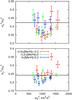
Fig. 3 Properties of the velocity ellipsoid from the RAVE data. The squared axis ratios of the velocity ellipsoid
 and
as a
function of J − K are plotted. The mean
values are marked by horizontal lines.
and
as a
function of J − K are plotted. The mean
values are marked by horizontal lines. -
3.
The Hipparcos sample is restricted to completeness limits in V magnitude bins and supplemented by the Catalogue of Nearby Stars (CNS4) to have a better representation of the faint end of the main sequence, as discussed in Just & Jahreiß (2010), with a total of N = 2176 stars. The stars have Johnson B and V photometry, vr, μ, and parallaxes. The sample is binned according to absolute magnitude in V.
-
4.
The last data set is a sample of McCormick K and M dwarfs with stellar ages determined by atmosphere activities (Vyssotsky 1963). It contains 516 stars with reliable distances and space velocity components. The sample is binned in stellar age.
3. Jeans analysis
The asymmetric drift is governed by the Jeans equation (Binney & Tremaine 2008),  (2)with tracer density
ν and covariance
(2)with tracer density
ν and covariance  .
Roughly speaking, it expresses dynamical equilibrium in an axisymmetric system within a
volume element in a cylindrical coordinate system. The left-hand side represents the
difference of the gravitational force in the Galactic potential and the centrifugal force,
while the terms on the right-hand side represent dynamical pressure and shear forces acting
on the surfaces of the volume. There are two crucial assumptions for the validity of Eq.
(2), namely axisymmetry of the system and
dynamical equilibrium of the stellar population under consideration. The former assumption
can be broken by a spiral density wave, while the latter can be violated for young
populations, whose mean age is smaller than the epicyclic period.
.
Roughly speaking, it expresses dynamical equilibrium in an axisymmetric system within a
volume element in a cylindrical coordinate system. The left-hand side represents the
difference of the gravitational force in the Galactic potential and the centrifugal force,
while the terms on the right-hand side represent dynamical pressure and shear forces acting
on the surfaces of the volume. There are two crucial assumptions for the validity of Eq.
(2), namely axisymmetry of the system and
dynamical equilibrium of the stellar population under consideration. The former assumption
can be broken by a spiral density wave, while the latter can be violated for young
populations, whose mean age is smaller than the epicyclic period.
In Eq. (2) the radial gradient term can be
parameterised by the local radial scalelength
RE of  via
via
 . It is a composition of the
radial scalelength Rν of the tracer density
ν and Rσ of the radial
velocity dispersion
. It is a composition of the
radial scalelength Rν of the tracer density
ν and Rσ of the radial
velocity dispersion  related by
 .
.
The vertical gradient of the covariance
in Eq. (2) measures the orientation of the
principal axes of the velocity ellipsoid above and below the Galactic plane. We use the
parametrisation  ;
η = 0 corresponds to a horizontal orientation of the principal axes and
η = 1 to a spherical orientation.
;
η = 0 corresponds to a horizontal orientation of the principal axes and
η = 1 to a spherical orientation.
Finally, we replace vc and
by
v⊙, V⊙, and ΔV
and evaluate Eq. (2) at the solar position
R = R0. Re-arranging the terms and dividing
by 2v⊙ we find ![Mathematical equation: \begin{eqnarray} \label{nonlinear}V_\mathrm{a}&=&v_\mathrm{c}-\overline{v}_\mathrm{\phi}=\Delta V-V_\mathrm{\sun} \\ &=& \frac{\Delta V^2 - V_\mathrm{\sun}^2}{2v_\mathrm{\sun}} + \frac{\sigma_{R}^2}{2v_\mathrm{\sun}} \left(\frac{R_0}{R_{E}}-1 - \eta\left[1-\frac{\sigma_{z}^2}{\sigma_{R}^2}\right] + \frac{\sigma_\mathrm{\phi}^2}{\sigma_{R}^2}\right)\cdot \nonumber \end{eqnarray}](/articles/aa/full_html/2013/09/aa21559-13/aa21559-13-eq124.png) (3)This
is the non-linear equation for the asymmetric drift Va as
function of for a set of
stellar subpopulations. It connects the measured mean tangential velocity
(3)This
is the non-linear equation for the asymmetric drift Va as
function of for a set of
stellar subpopulations. It connects the measured mean tangential velocity
 of a subpopulation
with respect to the Sun and the peculiar motion of the Sun V⊙.
There are two types of non-linearity on the right-hand side of Eq. (3). The two quadratic terms
ΔV2 and
of a subpopulation
with respect to the Sun and the peculiar motion of the Sun V⊙.
There are two types of non-linearity on the right-hand side of Eq. (3). The two quadratic terms
ΔV2 and  yield a small
correction to the asymmetric drift with increasing significance of the first one with
increasing velocity dispersion (e.g. for the thick disc). This correction can easily be
taken into account. The second non-linearity is more crucial and occurs from a possible
variation of the radial scalelength and the shape and orientation of the velocity ellipsoid
for the different subpopulations introducing an additional dependence of the last bracket in
Eq. (3) on
σR.
yield a small
correction to the asymmetric drift with increasing significance of the first one with
increasing velocity dispersion (e.g. for the thick disc). This correction can easily be
taken into account. The second non-linearity is more crucial and occurs from a possible
variation of the radial scalelength and the shape and orientation of the velocity ellipsoid
for the different subpopulations introducing an additional dependence of the last bracket in
Eq. (3) on
σR.
Since the thickness of a stellar tracer population depends on the total surface density and the vertical velocity dispersion, a radially independent constant thickness requires a constant shape of the velocity dispersion ellipsoid to find Rσ = Rd, the scalelength of the total surface density. In the simplest case, where the radial scalelength of the tracer population Rν is the same, i.e. Rd = Rν = Rσ, we get Rν = 2RE in the asymmetric drift Eq. (3).
The impact of the orientation of the velocity ellipsoid via η in the Jeans equation is twofold. Since σz < σR, a spherical orientation (η = 1) results in a smaller asymmetric drift compared to a horizontal orientation with η = 0. On the other hand, a stellar population with a measured asymmetric drift Va requires a larger radial scalelength RE for η = 1 to fulfill the Jeans equation. For definiteness we adopt η = 1 (supported observationally and theoretically by Siebert et al. 2008; Binney & McMillan 2010) in the plots and interpretation of data, if necessary.
3.1. The linear Strömberg relation
In the standard application the quadratic terms ΔV2 and
in Eq. (3) are neglected and we find Strömberg’s
equation ![Mathematical equation: \begin{eqnarray} \label{stromberg} \Delta V&=&V_\mathrm{\sun}+\frac{\sigma_{R}^2}{k} \nonumber\\ k&=&2v_\mathrm{\sun} \left(\frac{R_0}{R_{E}}-1 - \eta\left[1-\frac{\sigma_{z}^2}{\sigma_{R}^2}\right] + \frac{\sigma_\mathrm{\phi}^2}{\sigma_{R}^2}\right)^{-1}\cdot \end{eqnarray}](/articles/aa/full_html/2013/09/aa21559-13/aa21559-13-eq133.png) (4)The
inverse slope k depends on the radial scalelength
RE and shape and orientation of the
velocity dispersion ellipsoid of the subpopulations with density ν. If we
assume that the shape and orientation of the velocity ellipsoids are the same, i.e.
(4)The
inverse slope k depends on the radial scalelength
RE and shape and orientation of the
velocity dispersion ellipsoid of the subpopulations with density ν. If we
assume that the shape and orientation of the velocity ellipsoids are the same, i.e.
 and same
η, and that the radial scalelength is the same for all subpopulations,
then k is the same for all subpopulations and thus independent of
σR. With these assumptions we end up with
the classical linear Strömberg relation, which we discuss in more detail in Sect. 4.1.
and same
η, and that the radial scalelength is the same for all subpopulations,
then k is the same for all subpopulations and thus independent of
σR. With these assumptions we end up with
the classical linear Strömberg relation, which we discuss in more detail in Sect. 4.1.
3.2. A new Strömberg relation
Since we have measurements of the shape of the velocity ellipsoid for each subsample, it
is useful to separate observables and unknowns in the non-linear asymmetric drift Eq.
(3) by rewriting it as  (5)with
 The
new quantity V′ contains corrections arising from the shape
and orientation of the velocity ellipsoid and the quadratic term
ΔV2. The quadratic term on the
right-hand side of Eq. (5) decreases the
zero point
V′(σR = 0) with
respect to the value of V⊙ by 1–2%. The new parameter
k′ depends only on the radial scalelength
RE of the stellar subpopulations. In the
new form of the Strömberg relation we need to assume only equal radial scalelengths for a
linear fit to the data to determine the peculiar motion of the sun
V⊙ by the zero point and
RE via the inverse slope
k′. In general, the scalelength
RE could be also a function of
σR, thus implying a dependence of
k′ on σR in Eq.
(5). It is discussed in detail in Sect.
4.3.
The
new quantity V′ contains corrections arising from the shape
and orientation of the velocity ellipsoid and the quadratic term
ΔV2. The quadratic term on the
right-hand side of Eq. (5) decreases the
zero point
V′(σR = 0) with
respect to the value of V⊙ by 1–2%. The new parameter
k′ depends only on the radial scalelength
RE of the stellar subpopulations. In the
new form of the Strömberg relation we need to assume only equal radial scalelengths for a
linear fit to the data to determine the peculiar motion of the sun
V⊙ by the zero point and
RE via the inverse slope
k′. In general, the scalelength
RE could be also a function of
σR, thus implying a dependence of
k′ on σR in Eq.
(5). It is discussed in detail in Sect.
4.3.
4. Results
We discuss first the application of the linear Strömberg relation on the RAVE data in comparison with the other data sets. In a second step we repeat the analysis with the RAVE data split into the metallicity bins and then apply the new Strömberg relation. In the third step we investigate in a more general frame the determination of the LSR and the radial scalelengths. Finally, we discuss a very simple toy model, which can reproduce our findings.
4.1. Standard analysis
In Fig. 4 we see that the linear Strömberg relation
(Eq. (4)) with constant slope
k-1 is poorly applicable to the RAVE data: the data points
are not following the same straight line. The formal best fit to the RAVE data (grey line
in Fig. 4) gives the LSR
V⊙ = −1.0 ± 2.1 km s-1, which is not consistent
with V⊙ = 5.25 ± 0.54 km s-1 obtained by Aumer & Binney (2009) by a similar linear fit to
Hipparcos data. The corresponding slope k = 58 km s-1 is
bigger than the classical value. An application of Eq. (4) with the mean ratios of the squared velocity dispersions
( and
and
 , see
Fig. 3) results in a short radial scalelength of
Rd = 2RE = 1.65 ± 0.16 kpc.
, see
Fig. 3) results in a short radial scalelength of
Rd = 2RE = 1.65 ± 0.16 kpc.
The SEGUE G dwarfs allow us to get only one significant point in the plot, and this point is consistent with the trend obtained from RAVE, while SEGUE M dwarfs seem to be off the trend. The M dwarf sample may suffer from biases in the distance determination. The local stars from the Hipparcos, CNS4, and McCormick samples are also generally consistent with the best-fitting line for RAVE, except for the two dynamically coldest bins. This feature, which was already observed by Dehnen & Binney (1998), could be explained by the fact that the young stars have not yet reached dynamical equilibrium.
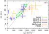 |
Fig. 4 Asymmetric drift for different data sets. The two black circles on the ΔV axis correspond to the different LSRs with V⊙ = 5.25 km s-1 from Aumer & Binney (2009) and V⊙ = 12.24 km s-1 from Schönrich et al. (2010) respectively. The grey line gives the best fit to the data points for RAVE dwarfs. It corresponds to the LSR V⊙ = −1.04 km s-1 and the scalelength of the disc Rd = 1.65 kpc. |
Overall, the SEGUE G dwarfs and the Hipparcos data support the slope k-1 determined by the RAVE data but with much larger scatter. The McCormick stars, the SEGUE M dwarfs, and the CNS4 data suggest a much smaller slope and larger LSR value, which would be inconsistent with the RAVE sample but support the large LSR value claimed by Schönrich et al. (2010). The increase of the observed Va (or equivalently ΔV) in Fig. 4 for the smallest velocity dispersions is inconsistent even with the model by Schönrich et al. (2010), suggesting non-equilibrium of the young subpopulation.
4.2. Metallicity dependence
Iin the Hipparcos sample a non-linear trend of the asymmetric drift with increasing velocity dispersion has already been observed. This is a sign that the radial scalelength is different for different subpopulations. Numerical models of Milky-Way-like galaxies also predict a systematic variation of the asymmetric drift with age and/or metallicity (e.g. Schönrich et al. 2010; Loebman et al. 2011). Schoenrich & Binney (2009a,b) have shown that radial mixing leads to a slight increase of the radial scalelength with increasing age. In Lee et al. (2011b) it was shown for the SEGUE G dwarf sample that the asymmetric drift in the thin disc decreases with decreasing metallicity in contrast to the naive expectation of local evolution models. Bovy et al. (2012a) also used the full SEGUE G dwarf sample (dominated by stars with | z| > 500 pc) to derive radial scalelengths of mono-abundance subpopulations. They found a significantly smaller radial scalelength for thick disc stars compared to thin disc stars, with a hint of decreasing scalelength with increasing metallicity inside the thin disc.
The RAVE sample in Fig. 4 also shows a systematic
non-linear trend, which may be due to a varying mixture of different populations with
different scalelengths. Binning stars of the RAVE sample in metallicities allow us to see
more interesting features in the behaviour of the asymmetric drift. Figure 2 shows that there is a systematic trend in both the
velocity dispersion and the asymmetric drift with metallicity, which is in part due to the
bluer colour of more metal-poor stars. In the top panel of Fig. 5 we plot the mean rotational velocity ΔV versus its
squared radial velocity dispersion for the three
different metallicity bins,
−0.5 < [M/H] < −0.2,
−0.2 < [M/H] < 0,
and
0 < [M/H] < 0.2. We
see that stars at different metallicities demonstrate different asymmetric drifts, with
more metal-poor stars having smaller asymmetric drifts and thus larger rotational
velocities. For comparison the RAVE data from Fig. 4
are replotted in grey to demonstrate that the non-linearity is partly resolved by the
separation into metallicity bins.
The common LSR V⊙ and the three inverse slopes
k for each metallicity bin are the free parameters for a joint linear
fit of the asymmetric drift Eq. (4). In the
top panel of Fig. 5 the best joint linear fit is
shown. We find for the LSR V⊙ = 2.52 ± 0.80 km s-1,
which is consistent with the estimate from Fig. 4.
The radial scalelengths of the three metallicity components can be estimated from the
inverse slopes k by inserting the mean ratios of the squared velocity
dispersions ( and
and
 , for
the low, intermediate, and high metallicity sample respectively). The radial scalelengths
are 2.73 ± 0.17, 1.97 ± 0.10, and 1.50 ± 0.05 kpc with increasing
metallicity, assuming
Rν = Rσ.
The decreasing radial scalelength with increasing metallicity corresponds to a negative
radial metallicity gradient because the fraction of metal-poor stars increases with
increasing radius.
, for
the low, intermediate, and high metallicity sample respectively). The radial scalelengths
are 2.73 ± 0.17, 1.97 ± 0.10, and 1.50 ± 0.05 kpc with increasing
metallicity, assuming
Rν = Rσ.
The decreasing radial scalelength with increasing metallicity corresponds to a negative
radial metallicity gradient because the fraction of metal-poor stars increases with
increasing radius.
Now we relax the assumption of similar velocity dispersion ellipsoids of the different
colour-metallicity bins and apply the new Strömberg relation derived in Eq. (5). In the bottom panel of Fig. 5, V′ as function of
is plotted.
All data points are shifted up by a few km s-1, but the general picture does
not change. The inverse slopes k′ of the joint linear
regression are now a direct measure of the radial scalelengths of the stellar populations
in the different metallicity bins. We find for the LSR
V⊙ = 3.06 ± 0.68 km s-1 slightly larger than the
previous value. The radial scalelengths of the disc are 2.91 ± 0.16, 2.11 ± 0.09, and
1.61 ± 0.05 kpc with increasing metallicity. The systematically larger radial scalelengths
in the new analysis (bottom panel of Fig. 5) are
mostly due to the shift of the LSR. The similarity of the classical and new analysis
demonstrates the small impact of the velocity ellipsoid compared to the radial scalelength
term in the asymmetric drift equation. Adopting a horizontal orientation of the velocity
dispersion ellipsoid η = 0 in Eq. (4) yields slightly larger scalelengths of 3.11 ± 0.23, 2.18 ± 0.12, and
1.62 ± 0.23 kpc respectively.
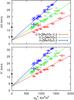 |
Fig. 5 The asymmetric drift for the RAVE dwarfs separated into three metallicity bins: −0.5 < [M/H] < −0.2, −0.2 < [M/H] < 0, and 0 < [M/H] < 0.2. The two black circles on the y-axis correspond to the LSR from Aumer & Binney (2009) and from Schönrich et al. (2010). The full lines show the best joint linear fit. Top: using Eq. (4). Bottom: using Eq. (5). The RAVE data without metallicity split of Fig. 4 are replotted with grey points. |
We can use these radial scalelengths to estimate the metallicity gradient in the disc. We assume the disc to consist of three populations, whose densities are described by exponentials with the corresponding scalelengths. Their metallicities are assumed to be −0.35, −0.1, and 0.1, which are median metallicities of the adopted bins. Relative weights of the populations at the solar radius are taken proportional to the total number of stars in the corresponding bins (see Table 2). We get a shallow radial metallicity gradient of −0.016 ± 0.002 dex kpc-1. To reproduce the observed metallicity gradient of −0.051 ± 0.005 dex kpc-1 (Coşkunoğlu et al. 2012), a much larger range of radial scalelengths or metallicities is required.
4.3. The LSR and radial scalelengths
In the previous analysis, we still adopted the same radial scalelength in each
metallicity bin independent of the colour J − K and thus
of the velocity dispersion. If we also relax this assumption, as suggested in the
literature mentioned in Sect. 4.2, then it is no
longer possible to determine the LSR (i.e.V⊙) by a linear
extrapolation to  . For
any extrapolation we would need a prediction of the dependence
. For
any extrapolation we would need a prediction of the dependence
 , e.g. from a model.
Instead we may adopt a value for V⊙ and derive individual radial scalelengths RE(ν) for each data point by determining the parameter k′(ν). The parameter k′(ν) corresponds to the inverse slope of the line connecting the data point with the zero point of Eq. (5). This is demonstrated in Fig. 6 for a few data points and the LSR of Aumer & Binney (2009, full black lines) compared to that of Schönrich et al. (2010, dashed black lines). The connecting lines are no longer linear fits to data but a visualization of k′(ν) from the application of Eq. (5) to each data point. Lifting the LSR value results in larger k′(ν) (smaller slopes) for all subsamples, leading to larger radial scalelengths from Eq. (7).
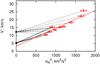 |
Fig. 6 Same data for the low-metallicity bin as in the bottom panel of Fig. 5. The two black circles on the y-axis correspond to the LSR from Aumer & Binney (2009) and from Schönrich et al. (2010). The full and dashed lines indicate for some subsamples the individual slopes and their dependence on the adopted LSR values, which are proportional to the inverse radial scalelengths. |
Figure 7 shows the variation of the radial scalelength as a function of colour J − K for the different metallicity bins, adopting the best-fit value for the solar motion V⊙ = 3.06 km s-1. For the higher metallicity bins, the data are consistent with a constant radial scalelength for all stars along the main sequence. In the low-metallicity bin a significant decline of Rd with the mean age of the stars is obvious in the sense of larger radial scalelength for the young metal-poor subpopulation.
The left-hand panels of Fig. 8 show the inverse
radial scalelengths for all RAVE subpopulations adopting the best fit LSR
V⊙ = 3.06 km s-1 (top panel), and the LSR of
Aumer & Binney (2009) (middle panel) and
Schönrich et al. (2010) (lower panel), with
colour-coded metallicity. The right-hand panels show the corresponding radial scalelengths
Rν = Rσ.
Since the LSR of Schönrich et al. (2010) is larger
than some V′ values, negative values corresponding to a
radially increasing density appear. More precisely, the scalelength
RE of
 becomes negative,
meaning an increasing radial energy density with increasing distance to the Galactic
centre (see Eq. (3)). This is physically
possible, for example, for metal-poor stars if the younger population born at larger radii
dominates over the older stars born further in.
becomes negative,
meaning an increasing radial energy density with increasing distance to the Galactic
centre (see Eq. (3)). This is physically
possible, for example, for metal-poor stars if the younger population born at larger radii
dominates over the older stars born further in.
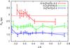 |
Fig. 7 Radial scalelengths corresponding to the best fit in different bins, calculated for the LSR V⊙ = 3.06 km s-1. Horizontal dashed lines represent the radial scalelengths used in the best fit in the lower panel of Fig. 5. |
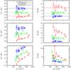 |
Fig. 8 Left panels: inverse radial scalelengths for all subpopulations adopting the LSR V⊙ = 3.06 km s-1 (best fit in the lower panel of Fig. 5, top panel), 5.25 km s-1 (Aumer & Binney 2009, middle panel), and 12.24 km s-1 (Schönrich et al. 2010, lower panel) with colour-coded metallicity. Right panels: radial scalelengths for the same data. For the Schönrich value of the LSR (lower panel), the absolute values | Rν | are plotted in logarithmic scale with negative values marked as crosses. |
We observe in both cases that the radial scalelengths are systematically larger for
smaller metallicity. But the trend in each metallicity bin as a function of
depends
sensitively on the adopted value for the LSR.
4.4. A simple model
There is a dynamical connection between radial gradients in the disc and the asymmetric drift due to the epicyclic motion of stars on non-circular orbits. Stars with guiding radii further in show a smaller tangential velocity in the solar neighbourhood because of the vertical component of angular momentum conservation. A negative radial density gradient results in a larger fraction of stars coming from the inner part of the disc compared to the outer part. Therefore the mean tangential velocity is smaller than the local circular velocity, corresponding to a positive asymmetric drift, and the distribution in vφ is skewed. Additionally, with increasing radial velocity dispersion the average distance to the guiding radius of stars in the solar neighbourhood increases, leading to an increasing asymmetric drift with increasing σR. As a second effect, a negative radial gradient in σR further increases the asymmetric drift and the skewness.
If there is a negative metallicity gradient in the Milky Way disc (e.g. as found by Coşkunoğlu et al. 2012, also using RAVE dwarfs), then a higher fraction of metal-rich stars observed in the solar neighbourhood is expected to possess guiding radii smaller than R0. It means that we are observing a larger asymmetric drift for these stars compared to more metal-poor stars at the same σR. In terms of Eq. (4) it means that metal-rich stars are more centrally concentrated and have a smaller disc scalelength Rν, while metal-poor stars have a bigger scalelength Rν. Any mixing process (by the epicyclic motion, radial migration due to orbit diffusion, or resonant scattering) tends to smear out gradients and increase the local scatter.
We demonstrate that a simple evolutionary model of the extended solar neighbourhood
combining the metal enrichment and a radial metallicity gradient can reproduce a
decreasing radial scalelength with increasing metallicity consistent with the observed
asymmetric drift. We adopt
SFR(R,t) ∝ exp(−R/Rd)
and constant in time t, the age velocity dispersion relation AVR with
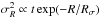 , and metal enrichment
[M/H](R,τ) = const. + Mττ + MRR ± Δ[M/H]
linear in age τ and in radius and allowing for a metallicity scatter.
With Monte Carlo realisations for each parameter set, we calculate the asymmetric drift
and velocity dispersion for each age-metallicity bin. The result of the best-fitting
parameter set with
(Rd,Rσ,Mτ,MR,Δ [M/H] ) = (1.8
kpc, 1.5 kpc, 0.04 dex Gyr-1, –0.07 dex kpc-1, 0.18 dex) is shown in
Fig. 9. Even though this plot is not enough to
tightly constrain all free parameters of the model, it is educating to see how easily the
observed metallicity trend can emerge.
, and metal enrichment
[M/H](R,τ) = const. + Mττ + MRR ± Δ[M/H]
linear in age τ and in radius and allowing for a metallicity scatter.
With Monte Carlo realisations for each parameter set, we calculate the asymmetric drift
and velocity dispersion for each age-metallicity bin. The result of the best-fitting
parameter set with
(Rd,Rσ,Mτ,MR,Δ [M/H] ) = (1.8
kpc, 1.5 kpc, 0.04 dex Gyr-1, –0.07 dex kpc-1, 0.18 dex) is shown in
Fig. 9. Even though this plot is not enough to
tightly constrain all free parameters of the model, it is educating to see how easily the
observed metallicity trend can emerge.
5. Discussion
The extended, kinematically unbiased catalogue of RAVE stars provides a very good tool to
analyse stellar dynamics in the solar neighbourhood and to study the asymmetric drift. We
analysed dwarf stars selected by a colour-dependent magnitude cut. The observed dependence
of the asymmetric drift velocity Va on the squared radial
velocity dispersion is
substantially non-linear, and the linear Strömberg relation fails to give a reasonable
approximation of the data. A somewhat similar analysis of the RAVE data was performed by
Coşkunoğlu et al. (2011). The authors used a
kinematically selected sample of stars with photometric distances to determine the velocity
of the Sun with respect to the neighbouring stars. The mean velocity of the Sun of about 13
km s-1 with respect to the local stars determined by Coşkunoğlu et al. (2011) is consistent with the mean ΔV
for the RAVE stars in Fig. 4. However, Coşkunoğlu et al. (2011) could not decompose this
velocity into the peculiar velocity of the Sun with respect to the LSR and the asymmetric
drift, which is the velocity of the LSR with respect to the mean velocity of stars in their
sample. Therefore they did not derive V⊙ but only
(V⊙ + Va), in contrast to their
suggestion.
When splitting the RAVE sample into three metallicity bins, the non-linearity of the asymmetric drift is reduced in each metallicity bin and a joint best linear fit confirms the low peculiar velocity of the Sun V⊙ = 2.52 ± 0.80 km s-1. The slopes of the asymmetric drift yield radial scalelengths of 2.73 ± 0.17, 1.97 ± 0.10, and 1.50 ± 0.05 kpc with increasing metallicity using the average values for the velocity dispersion shape.
For modern large samples like RAVE and SDSS/SEGUE, space velocities are available by
combining the survey data with distance estimates and proper motion catalogues. Therefore
the velocity dispersion ellipsoid is available for each stellar subsample, and we propose to
rearrange the Jeans equation in such a way that all measured contributions are combined on
the left-hand side to V′. This leads to an improved asymmetric
drift equation (Eq. (5)). In this new
Strömberg equation, the only unknown is the radial scalelength
RE of
, which determines the
slope of V′ as function of
. This new
equation allows a cleaner investigation of the interrelation of radial scalelengths and the
adopted (or determined) LSR (i.e. the peculiar motion of the Sun
V⊙).
We applied the new Strömberg equation to the RAVE data split in the metallicity bins. The best joint linear fit gives a value V⊙ = 3.06 ± 0.68 km s-1 for the LSR. The radial scalelengths are 2.91 ± 0.16, 2.11 ± 0.09, and 1.61 ± 0.05 kpc respectively for the metallicities [M/H] = –0.35, –0.1, and +0.1 dex in the disc. Adopting a horizontal orientation of the velocity ellipsoids above and below the midplane yield 10–20 percent larger scalelengths. The small differences of the new and old Strömberg equations show that the contribution of the velocity ellipsoid terms to the asymmetric drift are less significant, the overall trend of the asymmetric drift is dominated by the disc scalelengths and variations of it. The radial scalelength of the disc is smaller for higher metallicities, implying a more centrally concentrated distribution of metal-rich stars. The dependence of the asymmetric drift on metallicity can serve as a good constraint for chemodynamical models of the Milky Way and for the effect of radial migration on the stellar dynamics and abundance distribution in the solar neighbourhood.
If the radial scalelengths of the subpopulations are different for different velocity
dispersions, the new Strömberg equation Eq. (5) is still applicable, but now the inverse slope k′
is no longer constant but depends on the squared velocity dispersion
of the
subpopulation. The thus observed or theoretically predicted asymmetric drift and velocity
dispersions serve us as a measure of k′ on the right-hand side
of Eq. (5), corresponding to the inverse
radial scalelength RE of
if the peculiar
motion of the Sun V⊙ is known. In addition to the overall trend
of larger radial scalelengths for lower metallicities, we find within the metal-poor bin a
trend of decreasing scalelength with increasing velocity dispersion. This can be a hint of
an increasing contribution of thick disc stars combined with a small thick disc radial
scalelength. Alternatively, it is the contribution of a young metal-poor subpopulation of
the thin disc with large radial scalelength (Fig. 7).
The inverted trend of faster rotation for more metal-poor stars, at least in the younger
thin disc, as observed in Lee et al. (2011b), Liu & van de Ven (2012), Loebman et al. (2011), can be dynamically understood by the rule: lower
metallicity → larger velocity dispersion and larger radial scalelength → smaller asymmetric
drift → faster mean rotation. The chemodynamical model by Schönrich et al. (2010) probably can be interpreted in these terms. Each point of
the non-linear dependence from Schönrich et al. (2010) should correspond by Eq. (5) via its own k′ to
the radial scalelength RE. Therefore, the
dependence from Schönrich et al. (2010) can be interpreted as an increase of
Rν and/or
Rσ with the velocity dispersion
σR of the subpopulations. We have shown that
elevating V⊙ to 12 km s-1 results in significantly
increased radial scalelengths, which are even negative for some low-metallicity bins. The
physical interpretation of an increasing pressure with radius is
questionable. A second effect of a larger LSR value is a systematic trend of decreasing
scalelength with increasing velocity dispersion. This is counterintuitive to the impact of
radial migration, which should flatten radial gradients with increasing age and velocity
dispersion.
Another possible explanation for the discrepancies in the determination of the LSR are
non-axisymmetric features. A local spiral wave perturbation, which could influence the
stellar dynamics in the solar neighbourhood, can account for an offset of ≈6
km s-1 (Siebert et al. 2012). It would
break the axisymmetry of the gravitational potential required by Eq. (2), thus making all further analysis
inapplicable. The dynamically coldest subpopulations of stars are the most susceptible to
small gravitational perturbations, while dynamically hotter subpopulations are less affected
by them. Thus a Jeans analysis could break down for small
while still
being a good approximation for big . This would
apply to the bluest bins of the Hipparcos sample and also to the maser measurements of
star-forming regions. There is still no precise model to correct for these effects in the
solar neighbourhood.
From the slope of the asymmetric drift dependence on the radial velocity dispersion, we can
estimate the radial scalelength RE of
in the Galactic disc.
With  and the standard assumption
Rσ = Rν,
we get Rν ranging from 2.9 kpc to 1.6 kpc. If
Rσ is significantly larger than
Rν, as assumed by Bienaymé (1999), then Rν can
be smaller than our estimate by up to a factor of two, falling well below 2 kpc.
and the standard assumption
Rσ = Rν,
we get Rν ranging from 2.9 kpc to 1.6 kpc. If
Rσ is significantly larger than
Rν, as assumed by Bienaymé (1999), then Rν can
be smaller than our estimate by up to a factor of two, falling well below 2 kpc.
The orientation of the velocity ellipsoid measured by the vertical gradient of
has a minor impact on the radial scalelength. With η → 0 (horizontal
orientation), the scalelength RE would increase
by less than 20%. The new Stömberg relation (see Eq. (5)) shows that a re-determination of the velocity ellipsoid has, in
general, a small effect on the determination of the LSR and the radial scalelengths.
Based on the large data sample of RAVE dwarfs, we have demonstrated that the Jeans equation
is problematic for the determination of both the LSR (i.e. the tangential peculiar motion of
the Sun V⊙) and the radial scalelengths of the stellar
populations simultaneously. The extrapolation to the asymmetric drift value at
σR = 0 depends sensitively on the sample
selection and on additional assumptions. On the other hand, the Jeans equation provides a
sensitive tool to test Milky Way models on their dynamical consistency. The LSR value cannot
be adjusted independently because any variation has a large impact on the radial
scalelengths of all stellar populations in dynamical equilibrium. Dynamically, the radial
scalelength RE of the radial energy density
is relevant, and its
split into the scalelengths of the density and of the velocity dispersion needs further
information, such as the vertical thickness in combination with the shape of the velocity
dispersion ellipsoid.
Acknowledgments
O.G. acknowledges funding by International Max Planck Research School for Astronomy & Cosmic Physics at the University of Heidelberg. This work was supported by Sonderforschungsbereich SFB 881 “The Milky Way System” (subproject A6) of the German Research Foundation (DFG). Funding for RAVE has been provided by: the Australian Astronomical Observatory; the Leibniz-Institut für Astrophysik Potsdam (AIP); the Australian National University; the Australian Research Council; the French National Research Agency; the German Research Foundation (SPP 1177 and SFB 881); the European Research Council (ERC-StG 240271 Galactica); the Istituto Nazionale di Astrofisica at Padova; The Johns Hopkins University; the National Science Foundation of the USA (AST-0908326); the W. M. Keck foundation; the Macquarie University; the Netherlands Research School for Astronomy; the Natural Sciences and Engineering Research Council of Canada; the Slovenian Research Agency; the Swiss National Science Foundation; the Science & Technology Facilities Council of the UK; Opticon; Strasbourg Observatory; and the Universities of Groningen, Heidelberg, and Sydney. The RAVE web site is at http://www.rave-survey.org. Funding for SDSS-I and SDSS-II has been provided by the Alfred P. Sloan Foundation, the Participating Institutions, the National Science Foundation, the US Department of Energy, the National Aeronautics and Space Administration, the Japanese Monbukagakusho, the Max Planck Society, and the Higher Education Funding Council for England. The SDSS Web Site is http://www.sdss.org/. The authors are very grateful to Young-Sun Lee and Timothy C. Beers for providing their SEGUE data sample for our analysis and for fruitful discussions, as well as to Hartmuth Jahreiß for providing us with results of his analysis of the local stellar samples. We thank the anonymous referee for valuable comments and the language editor for improving the English language.
References
- Aumer, M., & Binney, J. 2009, MNRAS, 397, 1286 [NASA ADS] [CrossRef] [Google Scholar]
- Bienaymé, O. 1999, A&A, 341, 86 [NASA ADS] [Google Scholar]
- Binney, J. 2010, MNRAS, 401, 2318 [NASA ADS] [CrossRef] [Google Scholar]
- Binney, J., & McMillan, P. 2010, MNRAS, 413, 1889 [Google Scholar]
- Binney, J., & Tremaine, S. 2008, Galactic Dynamics (Princeton: University Press) [Google Scholar]
- Boeche, C., Siebert, A., Williams, M., et al. 2011, AJ, 142, 193 [NASA ADS] [CrossRef] [Google Scholar]
- Bochanski, J. J., Hawley, S. L., & West, A. A. 2011, AJ, 141, 98 [NASA ADS] [CrossRef] [Google Scholar]
- Bovy, J., Rix, H.-W., Liu, C., et al. 2012a, ApJ, 753, 148 [NASA ADS] [CrossRef] [Google Scholar]
- Bovy, J., Allende Prieto, C., Beers, T., et al. 2012b, ApJ, 759, 131 [NASA ADS] [CrossRef] [Google Scholar]
- Burnett, B., Binney, J., Sharma, S., et al. 2011, A&A, 532, A113 [NASA ADS] [CrossRef] [EDP Sciences] [Google Scholar]
- Chiappini C., Matteucci F., & Romano D. 2001, ApJ, 554, 1044 [NASA ADS] [CrossRef] [Google Scholar]
- Coşkunoğlu, B., Ak, S., Bilir, S., et al. 2011, MNRAS, 412, 1237 [NASA ADS] [Google Scholar]
- Coşkunoğlu, B., Ak, S., Bilir, S., et al. 2012, MNRAS, 419, 2844 [NASA ADS] [CrossRef] [Google Scholar]
- Dehnen, W., & Binney, J. 1998, MNRAS, 398, 387 [NASA ADS] [CrossRef] [Google Scholar]
- Gillessen, S., Eisenhauer, F., Fritz, T. K., et al. 2009, ApJ, 707, 114 [Google Scholar]
- Just, A., & Jahreiß, H. 2010, MNRAS, 402, 461 [NASA ADS] [CrossRef] [Google Scholar]
- Lee, Y. S., Beers, T. C., & Allen de Prieto, C. 2011a, AJ, 141, 90 [NASA ADS] [CrossRef] [Google Scholar]
- Lee, Y. S., Beers, T. C., An, D., et al. 2011b, ApJ, 738, 187 [NASA ADS] [CrossRef] [Google Scholar]
- Liu, C., & van de Ven, G. 2012, MNRAS, 425, 2144 [NASA ADS] [CrossRef] [Google Scholar]
- Loebman, S. R., Roskar, R., Debattista, V. P., et al. 2011, ApJ, 737, 8 [NASA ADS] [CrossRef] [Google Scholar]
- Matteucci, F., & Francois, P. 1989, MNRAS, 239, 885 [NASA ADS] [CrossRef] [Google Scholar]
- McMillan, P. J., & Binney, J. 2010, MNRAS, 402, 934 [NASA ADS] [CrossRef] [Google Scholar]
- Minchev, I., Chiappini, C., & Martig, M., 2013, A&A, in press, DOI: 10.1051/0004-6361/201220189 [Google Scholar]
- Reid, M. J. 1993, ARA&A, 31, 345 [NASA ADS] [CrossRef] [Google Scholar]
- Reid, M. J., & Brunthaler, A., 2005, Future Directions in High Resolution Astronomy, ASP Conf. Ser., 340, 253 [Google Scholar]
- Reid, M. J., Menten, K. M., Zheng, X. W., et al. 2009, ApJ, 700, 137 [NASA ADS] [CrossRef] [Google Scholar]
- Scannapieco, C., White, S. D. M., Springel, V., & Tissera, P. B. 2011, MNRAS, 417, 154 [NASA ADS] [CrossRef] [Google Scholar]
- Schönrich, R., & Binney, J. 2009a, MNRAS, 399, 1145 [NASA ADS] [CrossRef] [Google Scholar]
- Schönrich, R., & Binney, J. 2009b, MNRAS, 396, 203 [NASA ADS] [CrossRef] [Google Scholar]
- Schönrich, R., Binney, J., & Dehnen, W. 2010, MNRAS, 403, 1829 [NASA ADS] [CrossRef] [Google Scholar]
- Skrutskie, M. F., Cutri, R. M., Stiening, R., et al. 2006, AJ, 131, 1163 [NASA ADS] [CrossRef] [Google Scholar]
- Siebert, A., Bienaymë, Binney, J., et al. 2008, MNRAS, 391, 793 [NASA ADS] [CrossRef] [Google Scholar]
- Siebert, A., Famaey, B., Minchev, I., et al. 2011a, MNRAS, 412, 2026 [NASA ADS] [CrossRef] [Google Scholar]
- Siebert, A., Williams, M. E. K., Siviero, A., et al. 2011b, AJ, 141, 187 [NASA ADS] [CrossRef] [Google Scholar]
- Siebert, A., Famaey, B., Binney, J., et al. 2012, MNRAS, 425, 2335 [NASA ADS] [CrossRef] [Google Scholar]
- Steinmetz, M., Zwitter, T., Siebert, A., et al. 2011, AJ, 132, 164 [Google Scholar]
- Vyssotsky, A. N. 1963, in Stars and Stellar Systems, eds. K. A. Strand, Basic Astronomical Data (Chicago: Univ. Chicago press), 3, 120 [Google Scholar]
- West, A. A., Morgan, D. P., Bochanski, J. J., et al. 2011, AJ, 141, 97 [NASA ADS] [CrossRef] [Google Scholar]
- Wielen, R., Fuchs, B., Dettbarn, C. 1996, A&A, 314, 438 [NASA ADS] [Google Scholar]
- Yanny, B., Rockosi, C., Newberg, H. J., Knapp, G. R., & Adelman-McCarthy, J. K. 2009, AJ, 137, 4377 [NASA ADS] [CrossRef] [Google Scholar]
- Zwitter, T., Siebert, A., Munari, U., et al. 2008, AJ, 136, 421 [NASA ADS] [CrossRef] [Google Scholar]
- Zwitter, T., Matijevič, G., Breddels, M. A., et al. 2010, A&A, 522, A54 [NASA ADS] [CrossRef] [EDP Sciences] [Google Scholar]
All Tables
All Figures
|
Fig. 1 CMD of the full RAVE sample based on Zwitter distances. Surface gravity log g is colour-coded and the lines show the selected dwarf stars. |
| In the text | |
|
Fig. 2 Measured mean tangential velocity ΔV (full circles) and radial velocity dispersion σR (crosses) of the RAVE sample based on Zwitter distances as functions of J − K colour. |
| In the text | |
|
Fig. 3 Properties of the velocity ellipsoid from the RAVE data. The squared axis
ratios of the velocity ellipsoid |
| In the text | |
|
Fig. 4 Asymmetric drift for different data sets. The two black circles on the ΔV axis correspond to the different LSRs with V⊙ = 5.25 km s-1 from Aumer & Binney (2009) and V⊙ = 12.24 km s-1 from Schönrich et al. (2010) respectively. The grey line gives the best fit to the data points for RAVE dwarfs. It corresponds to the LSR V⊙ = −1.04 km s-1 and the scalelength of the disc Rd = 1.65 kpc. |
| In the text | |
|
Fig. 5 The asymmetric drift for the RAVE dwarfs separated into three metallicity bins: −0.5 < [M/H] < −0.2, −0.2 < [M/H] < 0, and 0 < [M/H] < 0.2. The two black circles on the y-axis correspond to the LSR from Aumer & Binney (2009) and from Schönrich et al. (2010). The full lines show the best joint linear fit. Top: using Eq. (4). Bottom: using Eq. (5). The RAVE data without metallicity split of Fig. 4 are replotted with grey points. |
| In the text | |
|
Fig. 6 Same data for the low-metallicity bin as in the bottom panel of Fig. 5. The two black circles on the y-axis correspond to the LSR from Aumer & Binney (2009) and from Schönrich et al. (2010). The full and dashed lines indicate for some subsamples the individual slopes and their dependence on the adopted LSR values, which are proportional to the inverse radial scalelengths. |
| In the text | |
|
Fig. 7 Radial scalelengths corresponding to the best fit in different bins, calculated for the LSR V⊙ = 3.06 km s-1. Horizontal dashed lines represent the radial scalelengths used in the best fit in the lower panel of Fig. 5. |
| In the text | |
|
Fig. 8 Left panels: inverse radial scalelengths for all subpopulations adopting the LSR V⊙ = 3.06 km s-1 (best fit in the lower panel of Fig. 5, top panel), 5.25 km s-1 (Aumer & Binney 2009, middle panel), and 12.24 km s-1 (Schönrich et al. 2010, lower panel) with colour-coded metallicity. Right panels: radial scalelengths for the same data. For the Schönrich value of the LSR (lower panel), the absolute values | Rν | are plotted in logarithmic scale with negative values marked as crosses. |
| In the text | |
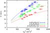 |
Fig. 9 Model predictions of a simple disc evolution model compared to the RAVE data shown in Fig. 8. |
| In the text | |
Current usage metrics show cumulative count of Article Views (full-text article views including HTML views, PDF and ePub downloads, according to the available data) and Abstracts Views on Vision4Press platform.
Data correspond to usage on the plateform after 2015. The current usage metrics is available 48-96 hours after online publication and is updated daily on week days.
Initial download of the metrics may take a while.