| Issue |
A&A
Volume 556, August 2013
|
|
|---|---|---|
| Article Number | A49 | |
| Number of page(s) | 9 | |
| Section | Stellar atmospheres | |
| DOI | https://doi.org/10.1051/0004-6361/201321909 | |
| Published online | 24 July 2013 | |
Spectral modelling of the α Virginis (Spica) binary system
1 Institut d’Astrophysique et de Géophysique, Université de Liège, Bât. B5c, Allée du 6 Août 17, 4000 Liège, Belgium
e-mail: This email address is being protected from spambots. You need JavaScript enabled to view it.
2 Instituto de Ciencias Físicas, Universidad Nacional Autónoma de México, Cuernavaca, 62210 Morelos, México
3 Institute for Astronomy, University of Hawaii, 2680 Woodlawn Drive, Honolulu, HI, 96822, USA
e-mail: This email address is being protected from spambots. You need JavaScript enabled to view it.
4 Instituto de Astronomía, Universidad Nacional Autónoma de México, México, D.F., México
e-mail: This email address is being protected from spambots. You need JavaScript enabled to view it.
Received: 17 May 2013
Accepted: 20 June 2013
Abstract
Context. The technique of matching synthetic spectra computed with theoretical stellar atmosphere models to the observations is widely used in deriving fundamental parameters of massive stars. When applied to binaries, however, these models generally neglect the interaction effects present in these systems.
Aims. The aim of this paper is to explore the uncertainties in binary stellar parameters that are derived from single-star models.
Methods. Synthetic spectra that include the tidal perturbations and irradiation effects are computed for the binary system α Virginis (Spica) using our recently-developed CoMBiSpeC model. The synthetic spectra are compared to S/N ~ 2000 observations and optimum values of Teff and log g are derived.
Results. The binary interactions have only a small effect on the strength of the photospheric absorption lines in Spica (<2% for the primary and <4% for the secondary). These differences are comparable to the uncertainties inherent to the process of matching synthetic spectra to the observations and thus the derived values of Teff and log g are unaffected by the binary perturbations. On the other hand, the interactions do produce significant phase-dependent line profile variations in the primary star, leading to systematic distortions in the shape of its radial velocity curve. Migrating sub-features (“bumps”) are predicted by our model to be present in the same photospheric lines as observed, and their appearance does not require any a priori assumptions regarding non-radial pulsation modes. Matching the strength of lines in which the most prominent “bumps” occur requires synthetic spectra computed with larger “microturbulence” than that required by other lines.
Key words: stars: massive / binaries: general / stars: fundamental parameters / stars: atmospheres / binaries: spectroscopic / stars: individual:αVirginis
Current address: Instituto de Astronomía, UNAM, Apdo. Postal 70-264, México D.F., México, e-mail: This email address is being protected from spambots. You need JavaScript enabled to view it.
© ESO, 2013
1. Introduction
Massive stars play a key role in the evolution of galaxies through their high luminosity, powerful winds, heavy element enrichment of the ISM, and the explosions when they end their lives as supernovae. The importance of determining their fundamental parameters cannot be overstated, and considerable effort has been invested in obtaining high quality observations and applying theoretical stellar structure models to establish these parameters (see for example, Evans et al. 2011; Martins 2011; Massey et al. 2009; 2012). Although significant progress has been made, there are still some important gaps in our understanding of the physical processes that govern the structure and evolution of massive stars. One of these gaps involves the effects caused by a binary companion on the emergent spectrum, from which the fundamental parameters are generally derived.
Binary systems provide the only direct means of determining the masses of stars and thus they are used to test the models of stellar structure which are then applied to single stars. The usual method for obtaining the binary star parameters is through the use of the radial velocity (RV) curves and model atmosphere codes. This yields a lower limit to the masses of the two stars, msin3i, the stellar radii R, effective temperature Teff, surface gravitational acceleration log g, and metallicity (see, for example, Massey et al. 2012).
The majority of stellar atmosphere models have been developed for single stars. Thus, one of the important questions that arises concerns the extent to which they can be used to properly model binary stars since the latter are subject to a variety of interaction effects. For example, gravity darkening and irradiation of the hemisphere facing the companion are expected to lead to different Teff values over the surface, with analogous differences in log g values due to the tidal distortion. In addition, non-synchronous rotation and orbital eccentricity induce oscillations on the stellar surface that may lead to photospheric absorption line profiles that are significantly different from those that are predicted by single-star atmospheric models (Vogt & Penrod 1983). It is possible that the temporal variability of these line profiles can have a significant impact on the determination of the fundamental parameters through the distortion of the RV curves (Koenigsberger et al. 2012).
We have developed a method for computing the spectra of binary systems which takes into account interaction effects. In a first stage, the code was designed for circular massive binary systems (Palate & Rauw 2012) in which the distorted shape of the stellar surfaces due to the gravitational interaction is calculated and then the emergent spectra at different orbital phases are computed. In a second paper the method was extended to include eccentric binaries and to incorporate radiation pressure effects (Palate et al. 2013). This new version of the CoMBiSpeC (Code of Massive Binary Spectral Computation) now allows spectral computation of massive binary systems in general. In this paper we use this code to address the question of the extent to which the binary interactions may affect the outcome of the standard procedure of matching stellar atmosphere models to observations in order to derive values of Teff and log g. This exploratory investigation will focus on the nearby and well-studied binary system α Virginis (=Spica = HD 116658).
In this paper we use local line-profiles obtained from a full radiative transfer computation using the standard model atmosphere code TLUSTY. This enables us to analyse the effects of the binary interaction on the determination of Teff and log g, in addition to the line-profile variability. In Sect. 2 we provide a brief review of Spica’s properties; in Sect. 3 we describe the procedure that was followed to produce the synthetic spectra, in Sect. 4 we present the results, and in Sect. 5 the conclusion.
2. The Spica binary system
Spica is a double-lined, short-period (~4 days) spectroscopic binary in an eccentric orbit. The primary component is classified as B1.5 IV-V and based on early observations that disclosed a 4.17 h spectroscopic and photometric period, it was believed to be a β Cephei-type star (Shobbrook et al. 1969; 1972). However, the photometric variations seem to have vanished in 1970−1971 (Smith 1985a). On the other hand, the spectroscopic line-profile variations have persisted (Smak 1970; Smith 1985a,b; Riddle 2000; Harrington 2009). They are commonly described in terms of travelling “bumps” that migrate from the blue to the red wing of the weak photospheric absorption lines, but also include variations in the slope of the line wings. A periodicity of 6.5 and 3.2 h has been associated with these variations (Smith 1985a).
Spica was observed interferometrically by Herbison-Evans et al. (1971), allowing a direct determination of orbital separation, stellar radius of the primary (R1 = 8.1 ± 0.5 R⊙) and orbital inclination (i = 65.9° ± 1.8°), which when combined with RV curves yield the masses, M1 = 10.9 ± 0.9 M⊙ and M2 = 6.8 ± 0.8 M⊙. More recently, it was observed with the CHARA and SUSI interferometric arrays by Aufdenberg (2007) and collaborators. The analysis followed that of Herbison-Evans et al. (1971) except that the stellar disks were no longer assumed to be of uniform brightness but were assumed to be rotationally and tidally distorted. The results of this analysis were kindly provided to us by Aufdenberg (2008, priv. comm.) and consist of slightly different values for the stellar and orbital parameters. They are listed in Table 1 together with those of Herbison-Evans et al. (1971).
Spica parameters.
The stellar rotation velocities, vrot, were derived by Smith (1985a), who modelled the line-profile variability under the assumption that it could be described in terms of high-order non-radial pulsation modes. To derive the order of the modes, Smith (1985a) used a trial and error profile-fitting method in which he included the presence of travelling “bumps” and tested combinations of rotational, macroturbulent and pulsational velocities and periods. The rotation velocities he derived are v1sini = 161 ± 2 km s-1 and v2sini = 70 ± 5 km s-1.
Harrington et al. (2009) adopted the Aufdenberg et al. (2008) stellar and orbital parameters and Smith’s (1985a) values for vrot, and performed an ab initio calculation of the line profiles at several orbital phases in order to study the variability that is caused by the response of the star to tidal perturbations. The calculation involves the solution of the equations of motion of the surface elements in the presence of gravitational, Coriolis, centrifugal, viscous and gas pressure forces, and the projection of the resulting velocity field along the line of sight to the observer in order to compute photospheric absorption lines in the observer’s reference frame. Harrington et al. (2009) were able to reproduce the general trends in the line-profile variability and, in particular, the observed relative strength and number of “blue” to “red” migrating “bumps”. These “bumps” were found to arise in what Harrington et al. describe as “tidal flows”, a concept that differs from the non-radial pulsation representation in that the travelling waves on the stellar surface are a consequence entirely of the response of this surface to the forcing and restoring agents, the interior structure of the star playing no role. The line profile calculation performed by Harrington et al. (2009) was done for an arbitrary absorption line assuming that the local line profile at each location on the stellar surface has a Gaussian shape. Thus, their study was limited to the analysis of line-profile variability alone, and no comparison of the effects on different lines (particularly those used for temperature and gravity diagnostics) was possible.
3. Method of analysis
Synthetic spectra were produced for a binary system under the assumptions of a) no interaction effects; and b) tidal and irradiation effects. These spectra will henceforth be alluded to as “unperturbed” and “perturbed”, respectively. The detailed procedure for generating the synthetic spectra is described below.
Rotating and binary stars are deformed from spherical symmetry and thus the gravity darkening effects1 lead to a non-uniform value of effective temperature and gravity over the stellar surface. When synthetic spectra are produced from model atmosphere grids, they are characterized by the values of effective temperature and surface gravity at the pole. Thus, we refer to our models with the values of  and log gpole.
The synthetic spectra were compared with observational data that were obtained on 2008 March 15–28 at the Canada France Hawaii (CFHT) 3.6 m telescope with the ESPaDOns spectropolarimeter, which are thoroughly discussed in Harrington et al. (2009). They consist of high resolution spectra (R = 68 000) in the wavelength range λλ 3700−9200 Å with typical signal-to-noise ratio S/N ~ 2000.
The synthetic spectra were produced as follows:
-
Step 1: the stellar surface deformation and velocity field of both stars in the binary system are computed using the TIDES code. This requires prior knowledge of the stellar masses, radii and rotation velocity, as well as the full set of orbital parameters. The masses and radii are those given by Aufdenberg et al. (2008) taking into account the uncertainties quoted by these authors, the eccentricity is from Riddle (2000), and the longitude of periastron ωper = 255° is from Harrington et al. (2009). The output consists of displacements and velocities (both radial and azimuthal) for each surface element as a function of time. A full description of the TIDES calculation is provided in Moreno et al. (2011) and a detailed description of the calculations that were performed for Spica can be found in Harrington et al. (2009).
-
Step 2: we use the grid of stellar atmosphere models computed with TLUSTY (Lanz & Hubeny 2007) to produce emergent flux spectra with microturbulent speeds in the range vturb = 2−15 km s-1 using the routine SYNSPEC492. The set of spectra for the primary star in Spica covers Teff = 22 000 to 25 000 K and log g = 3.75 to 4.00, and for the secondary the corresponding ranges are 18 000–22 000 K and log g = 4.00 to 4.25. The metallicity of these models is Solar and the SYNSPEC49 calculation was performed using the NLTE option3.
-
Step 3: CoMBiSpeC is used to compute the temperature and gravity distributions and then is used to linearly interpolate and Doppler-shift the spectra obtained from the SYNSPEC49 calculation to obtain the emergent spectrum for each surface element of the star (i.e., the “local” line profile) and then the final synthetic spectrum is produced by integration over the entire stellar surface. The Doppler shift is performed using the velocity field computed by TIDES projected along the line-of-sight to the observer.
-
Step 4: observational data obtained at one orbital phase when the lines of the primary and secondary are well-separated are compared to the synthetic spectra computed for the various sets of
and log gpole at a similar orbital phase in order to determine the best match between the synthetic and observed photospheric lines. Preference is given to matching lines that are good Teff and log g diagnostics4 and, among these, those that lie in spectral regions where the uncertainties in the continuum normalization of the data are minimum. The atlas of Walborn & Fitzpatrick (1990) is used as a guide for the trends in He i, He ii and Si iii line strengths with increasing Teff and log g. For the present investigation, over 160 synthetic model spectra were tested against the observations. A “best match” of the synthetic spectrum to the observations is attained when synthetic spectra with adjacent values of and log gpole bracket the majority of observed spectral lines amongst the ones used for diagnostics purposes. As will be shown below, our best match synthetic spectra reproduce the observations to within ~5% of continuum unit.
We initiated the analysis using the orbital elements and stellar parameters derived by Aufdenberg et al. (2008) and the value of vsini from Smith (1985a). The primary reason for this choice is that these parameters were found by Harrington et al. (2009) to produce line-profile variability that most resembled the one observed. The qualitative nature of the line profile variations predicted by the TIDES code depends not only on masses, stellar radii and orbital parameters but also on vsini, the depth of the layer that is modelled in TIDES, ΔR/R1, and on the kinematical viscosity, ν of the material. An adequate combination of all of these parameters is required to achieve a satisfactory match to the observations. For the present analysis we fixed M1, M2, e, ΔR/R1, ν and the computational parameters required by TIDES to the values that were found by Harrington et al. to best reproduce the line-profile variability. The parameters that were varied are: R1, R2, i (orbital inclination), and the values of Teff and log g for the two stars.
After several iterations we found that the best fit to the observations was attained with  and i = 60°. Both of these values lie within the uncertainties quoted by Aufdenberg et al. (2008) and hence, we shall refer to the input parameter set as that of Aufdenberg et al. (2008).
We used the ESPaDOns spectra obtained on 22 and 26 March 2008 (orbital phases 0.88 and 0.84, respectively5) as the guide for the first synthetic spectrum, since at these orbital phases the absorptions arising in each star are well separated. The velocity field computed in Step 1 was applied to the grid of models described in Step 2 and the synthetic spectra (Step 3) were compared with these ESPaDOns spectra.
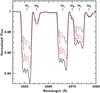 |
Fig. 1 Synthetic Si iii line profiles computed for Spica with the TLUSTY stellar atmosphere models for Teff and log g appropriate to each surface element and Doppler-shifted using the surface velocity field computed with TIDES. The three spectra correspond to microturbulent velocities vturb = 2 (dots), 10 (dashes) and 15 (continuous) km s-1 and illustrate how the larger values of this parameter produce greater line-strength in the Si iii λ 4552 line. The lines originating in the primary and secondary are indicated with m1, and m2 respectively. The depicted profiles correspond to orbital phase φ = 0.75. |
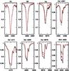 |
Fig. 2 Dependence of line strength on microturbulent speed vturb. As in Fig. 1, the same stellar atmosphere model computed with vturb = 2 (dots), 10 (dashes) and 15 (continuous) km s-1 is shown. The behaviour of the stronger He i lines is different from that of weaker lines. In the H-lines, the dependence on vturb is strongest in the line wings. |
In the initial iteration for finding the optimum values of , log gpole an excellent match was attained for the H and He i lines with vturb = 2 km s-1, but the majority of the heavy element lines were too weak by factors of 2–3. Thus, the next iteration consisted of finding the value of vturb for which the strength of the Si iii λλ 4552-4574 triplet lines coincided with the observations6. We found that a good match to the Si iii line strengths requires 10 ≤ vturb/(km s-1) ≤ 15, and the final model was computed with vturb = 15 km s-1. It must be noted, however, that this value of vturb resulted in lines such as O ii λλ 4072-79 being significantly stronger in the synthetic spectra than in the observations. Figure 1 illustrates the manner in which the Si iii triplet changes for vturb = 2, 10 and 15 km s-1, and Fig. 2 shows the effect on other lines. Noteworthy is the very different behaviour of He i λ 4471 from that of Si iii λ 4552 and other heavy-element lines. This difference may be traced to the atomic line-strength parameters which affect the shape of the line profiles.
Once the set of parameters that best described the ESPaDOnS spectrum of 22 March were determined, these were held constant and we proceeded to compute the synthetic spectra at 20 equally spaced orbital phases. These are the spectra that are discussed in the next sections.
4. Results
4.1. The impact of interaction effects on Teff and log g
The best match to the ESPaDOns spectra of 22 and 26 March was attained with (, log gpole) of (24000 ± 500 K, 3.78) for the primary and (19500 ± 500 K, 4.16) for the secondary. These values are in good agreement with those found by Aufdenberg et al. (2008) for the primary star, (24750 ± 500, 3.71 ± 0.06). For the secondary, our result is in agreement with Aufdenberg et al.’s log gpole = 4.16 ± 0.05, and Lyubimkov et al. (1995) = 20800 ± 1500 K.
The parameters of the final model are listed in Table 2, and selected spectral regions of these models and the corresponding observational data of 26 March (φ = 0.84) and 15 March (φ = 0.15) are shown in Figs. 3 and 4. Figures 5 and 6 illustrate the matching between observed and synthetic spectra for individual lines. The difference between the observed and the synthetic spectra is ≤5%, as shown by the plot at the bottom of these figures. For the 4060−4360 Å and 4360−4720 Å wavelength regions, the maximum difference is <4% except at λ 4078.4 (8.7%). For the 4730−5130 Å wavelength region, the maximum difference is 2.5% and appears in the wings of Hβ.
Parameters used for computation with the TIDES + CoMBiSpeC model.
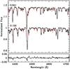 |
Fig. 3 Comparison of the best-fit CoMBiSpeC model (dots) with the ESPaDOns spectra of Spica at orbital phases 0.152 (15 March) and 0.841 (26 March; shifted by +0.2 continuum units). The tracing shown at the bottom is the difference between the 15 March spectrum and its corresponding synthetic spectrum and shows that the fit is good to ~3%. |
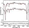 |
Fig. 4 Same as previous figure for the spectral region containing Hδ and Hγ. |
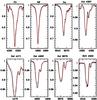 |
Fig. 5 Individual lines in the 26 March spectrum compared to the corresponding synthetic spectrum. |
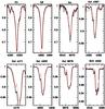 |
Fig. 6 Individual lines in the 28 March spectrum compared to the corresponding synthetic spectrum. |
The maximum departure from sphericity in Spica’s primary is ≤0.2 R⊙, and thus the value of log g over the stellar surface is practically constant. The largest Teff is found at the pole and decreases towards the equator, but the small gravity darkening leads to a Teff decrease of only ~500 K. The irradiation effect is also small and thus the hemisphere facing the secondary is nearly at the same temperature as the opposite hemisphere. The small differences in Teff and log g over the stellar surface in the primary lead to line strengths in the perturbed spectra that differ only slightly from those in the unperturbed spectrum. Figure 7 shows that the differences in the equivalent width (EW) of the lines in the perturbed and unperturbed spectra are ≤1.5%, which is below the typical observational uncertainties and those inherent to the spectrum fitting technique. Thus we conclude that despite the strong line-profile variability in Spica’s primary star, there is a negligible effect on the derivation of Teff and log g values.
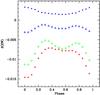 |
Fig. 7 Difference between equivalent widths measured on the perturbed and unperturbed spectra, Δ(EW) = [EWp − EWu] /EWu, of the primary star in Spica showing that the effects are ≤1.5%, and thus indicating that the interaction effects have a negligible impact on the spectral classification. Negative residuals indicate that the absorption in the perturbed profiles is weaker than in the unperturbed profiles. The different symbols correspond to: He i λ 4921(open triangles), He i λ 5875 (filled-in triangles), Si iii λ 4552 (stars) and Hβ (squares). |
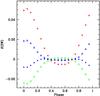 |
Fig. 8 Same as previous figure (Fig. 7) for the secondary showing that in this case, the effects are ≤5%. Note that around periastron, the Si iii λ 4552 strength increases by ~5% while that of Hβ decreases by ~2.5%. |
For the secondary, the effects caused by gravity darkening are also small, but due to the hotter primary the irradiation effects are more important. Hence, the largest Teff ~ 20 300 K is on the equator of the hemisphere facing the primary while the lowest Teff = 19 400 K occurs on the opposite hemisphere, also along the equator. The irradiated hemisphere of the secondary is viewed by the observer around periastron passage, at which time the EW of Si iii λ 4552 increases by ~5% while that of Hβ decreases by ~2%, as illustrated in Fig. 8.
It is interesting to note that despite the relatively small surface deformations, the observed light curve of Spica displays ellipsoidal variations (Shobbrook et al. 1969; Sterken et al. 1986) with peak-to-peak amplitudes ~0.03 mag. We computed the predicted light curve variations from out model results following the method described in Palate & Rauw (2012) and find a peak-to-peak amplitude ~0.02 mag. The difference between our predicted light curve and that which is observed may in part be due to the uncertainties introduced by the short-period photometric variability which is present in the observations.
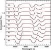 |
Fig. 9 Synthetic primary + secondary combined spectra of the Si iii triplet are stacked in order of increasing orbital phase (φ = 0 corresponds to periastron). The perturbed spectra are displayed with the dark tracing and the unperturbed spectra with dots. The “bumps” in the primary star’s perturbed profiles are evident as is the difficulty they introduce in properly locating the contribution of the secondary except at φ ~ 0.3 ± 0.05 and 0.8 ± 0.05 when the contribution from the secondary is clearly resolved. |
4.2. Line profile variability
The binary interactions significantly affect the shape of the line profiles. Figure 9 shows the Si iii triplet line profiles at 10 orbital phases in the perturbed and the unperturbed spectra. The strong phase-dependent variations in the perturbed profiles are clearly seen and can be described primarily in terms of “bumps” and asymmetries, similar to those present in the observational data7. The same behaviour is present in numerous other photospheric absorptions, such as He i λ 5875 (Fig. 10), but is at the ~1.5% level.
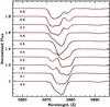 |
Fig. 10 Same as previous figure for He i λ 5875. |
The most prominent perturbations occur in absorption lines of intermediate intensity, as is shown in Fig. 11, where we plot the difference between the perturbed and unperturbed synthetic spectra at 10 phases in the orbital cycle for the λλ 4310−4580 Å region. Strong lines, such as Hγ, undergo weaker perturbations than lines such as He i λ 4471 and the Si iii triplet.
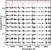 |
Fig. 11 Difference between the synthetic perturbed spectra of the primary and the corresponding unperturbed spectra showing that the lines of intermediate intensity display the most prominent variations in the “bump” structure. The orbital phases increase from bottom to top with increments of Δφ = 0.1 and starting with φ = 0. Differences are shifted along the vertical axis for clarity. The dotted tracing at the top is the perturbed spectrum at φ = 0.90, scaled and shifted to fit in this figure. |
4.3. Distortion of the RV curve
The line-profile variations introduce an intrinsic uncertainty in the RV measurements which, as will be shown below, leads to systematic distortions in the RV curve. To illustrate this point, the centroid of the lines He i λ 4921 and λ 5875, Si iii λ 4552 and Hβ were measured in the perturbed and unperturbed spectra by numerical integration between two fixed positions at the continuum level on both sides of the absorption minimum8.
Figure 12 shows the difference δ(RV) = (RV)p − (RV)u for the primary, where the subscripts “p” and “u” represent the perturbed and unperturbed spectra, respectively, and the RVu correspond to the actual orbital motion. The maximum semi-amplitudes of δ(RV) range between 6 and 10 km s-1, depending on the particular line being measured. A similar analysis performed using a cross-correlation method9 yields a semi-amplitude δ(RV) ~ 7 km s-1 for the two wavelength intervals that were cross-correlated (λλ 4150 − 4300 Å and λλ 5200 − 5800 Å), consistent with the result obtained for individual lines. The shape of the perturbed and unperturbed RV curves for He i λ 5875 is also shown in Fig. 12 (after scaling by a factor of 10 for illustration purposes) showing that the strongest distortion occurs on the ascending and descending branches of the RV curve, on both sides of the extrema; i.e., at orbital phases ~0.15, 0.40, 0.65 and 0.90. The combined effect of these distortions is to skew the RV curve, giving it the appearance of one with a larger eccentricity than that of the actual orbit.
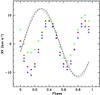 |
Fig. 12 Difference between RV measurements made on the perturbed and unperturbed spectra δ(RV) = (RV)p − (RV)u for He i λ 4921 (open triangles), He i λ 5875 (filled-in triangles), Si iii λ 4552 (stars) and Hβ (squares). Also shown is the shape of the perturbed (dash) and unperturbed (dots) RV curves for He i λ 5875 after down-scaling by a factor of 10 for illustration purposes. The perturbation leads to a RV curve corresponding to a more eccentric orbit than the actual orbit. |
For the secondary star, its weaker line-profile variability leads to much smaller deformations in the RV curves (see Fig. 13), δ(RV) = 2 km s-1, with extrema at φ ~ 0.2 and 0.85. The most strongly perturbed RV curve is that of Si iii λ 4552 due to the greater sensitivity of this line to the heating by irradiation of the companion.
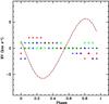 |
Fig. 13 As in the previous figure, the difference between RV measurements made on the perturbed and unperturbed spectra are plotted but here for the secondary star, and the scaled RV curves are those of Si iii λ 4552, which shows the strongest perturbation effects. |
4.4. Comparison of CoMBiSpeC and TIDES model line profiles
The CoMBiSpeC calculation uses the velocity field computed by TIDES to compute the line profiles. A line-profile calculation is also implemented in TIDES (Moreno et al. 2011) which in the original version employed in Harrington et al. (2009) assumed a Gaussian local line profile instead of a line profile generated from a stellar atmosphere calculation. In Fig. 14 we compare the line profiles produced by both calculations, but in this case TIDES uses a Voigt shape for the local line profiles with a Lorentzian coefficient aL = 0.3. Both calculations use the same surface velocity field (calculated by TIDES) and microturbulent speeds of 15 km s-1, and all the binary parameters are the same. The differences between the TIDES and the CoMBiSpeC calculations are minimal.
Because TIDES computes the line profile variability very rapidly, its use is desirable for the analysis of a large parameter space such as that involving stellar radius, rotation velocity, eccentricity, orbital inclination, layer depth and viscosity, and the above justifies its use for these purposes.
5. Summary and conclusions
In this paper we explore the uncertainties that binary interaction effects may introduce in the derivation of fundamental stellar parameters when using stellar atmosphere models constructed for single stars. Our test case is Spica, a relatively close B-type binary system with unevolved, detached components. We use the TIDES code to compute the surface deformation and velocity field, the TLUSTY model atmosphere synthetic spectral grids, and the CoMBiSpeC model to synthesize output spectra that include the effects of irradiation by the companion and the tidal perturbations. These synthetic spectra are compared to high S/N and high resolution observations from which the following results are derived:
-
1.
The phase-dependent variations in line strength (EW) due to the interactions is ≤2% for the primary and ≤4% for the secondary, leading to values of Teff and log g that are indistinguishable, within the uncertainties, from those derived from models that neglect the interactions. The reason for this is that the irradiation effects and the departure from sphericity of both stellar surfaces are very small. The radius of the secondary is ~7 times smaller than the orbital separation, so even though the primary is hotter, this large separation guarantees that only a small irradiation effect is present. Similar considerations apply to the tidal deformations. The radius of the primary is only ~3.6 times smaller than the orbital separation, but the irradiation from the secondary is insignificant due to its cooler temperature and, due to it’s smaller mass, the tidal deformations are also negligible.
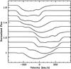
Fig. 14 The Si iii λ 4552 line profiles computed with ComBiSpeC compared with the line profiles computed with the TIDES code (dots). In this TIDES calculation, the computation is performed using Voigt local line profiles. The ComBiSpeC code uses the same velocity field that is computed with TIDES, but the local line profile is obtained from the non-LTE TLUSTY radiative transfer calculation. Only the profiles computed for the primary star are shown here.
-
2.
The primary star rotates super-synchronously, which significantly perturbs its surface, leading to strong phase-dependent line profile variations. As a result, the RV curve is distorted with respect to the curve that describes the orbital motion, with maximum deviations of ≤10 km s-1. Although the peak-to-peak amplitude of the RV curve is not affected, the shape is skewed so that a larger eccentricity than the actual value is inferred. We note that this effect may be the source of the discrepancy between the values of e that are given by Riddle (e = 0.067) and Herbison-Evans et al. (e = 0.146).
- 3.
The velocity structure that is computed by TIDES leads naturally to the presence of bumps on the profiles of lines such as the Si iii λλ 4552-72 triplet and other lines of intermediate strength without the need of any ad hoc assumption regarding non-radial pulsations. The nature of the bumps in the synthetic spectra is qualitatively similar to that in the observations for all lines contained in our spectra.
- 4.
The weaker lines in the spectrum require vturb = 10 − 15 km s-1, whereas He i lines such as λ 4471 and O ii favour a smaller value. Interestingly, the lines that show the clearest bumps are the ones that require the larger values of vturb to attain an adequate match to the line-strengths.
We conclude that for a binary system such as Spica, the uncertainties in the model-fitting process (NLTE effects, microturbulence, rectification of the continuum level in the observations) are larger than those introduced by the tidal velocity field and heating effects. Future work will extend the exploration introduced in this paper to systems with parameters that are different from Spica’s, where irradiation and tidal deformations are more important, in order to evaluate the uncertainties that are introduced in these cases with the use of single-star atmosphere models.
The above being said, it must be noted that nearly all of the synthetic model atmospheres are computed under the assumptions of hydrostatic and radiative equilibrium. However, the shear produced by different surface layers as they slide with respect to each other in response to the tidal perturbation leads to energy dissipation (Toledano et al. 2007; Moreno et al. 2011). Depending on the particular regions where this energy is deposited, the temperature structure of the outer layers may be altered with respect to that derived when radiative equilibrium is strictly enforced. Furthermore, the dynamical nature of the stellar photosphere could influence the assumptions that are used for fixing vturb, for example, assuming that it is constant over the stellar surface. A hint pointing towards a non-constant value of vturb is suggested by our results. Thus, the applicability of single-star models to close binary stars may need to be critically assessed.
As in Palate et al. (2013) we used a gravity darkening parameter equal to 0.25.
The grid of models is available at http://nova.astro.umd.edu/Tlusty2002/tlusty-frames-BS06.html and the latest version of SYNSPEC was obtained from http://nova.astro.umd.edu/Synspec49/synspec.html
It is important to note that the NLTE calculation is actually only performed on a limited number of the lines (mainly H, He and C N O in later stages). Lanz & Hubeny (2007) argue that NLTE effects in the other lines are small.
See, for example, Massey et al. (2009) for a more in-depth description of the spectrum-matching process.
The phase φ = 0 corresponds to the periastron passage of the observations and we used the T0 and the apsidal period derived by Aufdenberg et al. (2008).
An in-depth description of the manner in which vturb is generally determined may be found in Hunter et al. (2007). Included is a justification of the use of the Si iii triplet for fixing the value of this parameter as well as a discussion of the manner in which the use of different lines results in different values.
See Harrington et al. (2009) where a set of spectra computed at very short time steps and showing the moving “bumps” is illustrated.
The functional form is  , where xi, yi are the values of wavelength and flux at each wavelength step. The wavelength step of our synthetic spectra is 0.01 Å and integration intervals typically contained ~2000 points.
The FXCOR routine in the Image Reduction Analysis Facility (IRAF) package.
Acknowledgments
We wish to express our gratitude to Ivan Hubeny for guidance in the use and implementation of SYNSPEC49 and Andres Sixtos for performing the IRAF cross-correlation computation of the RVs. The authors also would like to acknowledge Jason Aufdenberg for a careful reading of this paper and helpful comments. We acknowledge support through the XMM/INTEGRAL PRODEX contract (Belspo), from the Fonds de Recherche Scientifique (FRS/FNRS); UNAM/DGAPA/PAPIIT grant IN-105313, and CONACYT grant 129343.
References
- Aufdenberg, J. 2007, AAS, 211, 6301 [NASA ADS] [Google Scholar]
- Evans, C. J., Taylor, W. D., Hénault-Brunet, V., et al. 2011, A&A, 530, A108 [NASA ADS] [CrossRef] [EDP Sciences] [Google Scholar]
- Harrington, D. M., Koenigsberger, G., Moreno, E., & Kuhn, J. 2009, ApJ, 704, 813 [NASA ADS] [CrossRef] [Google Scholar]
- Herbison-Evans, D., Hanbury, B. R., Davis, J., & Allen, L. R. 1971, MNRAS, 151, 161 [NASA ADS] [CrossRef] [Google Scholar]
- Hunter, I., Dufton, P. L., Smartt, S. J., et al. 2007, A&A, 466, 277 [NASA ADS] [CrossRef] [EDP Sciences] [Google Scholar]
- Koenigsberger, G., Moreno, E., & Harrington, D. M. 2012, A&A, 539, A84 [NASA ADS] [CrossRef] [EDP Sciences] [Google Scholar]
- Lanz, T., & Hubeny, I. 2007, ApJS, 169, 83 [CrossRef] [Google Scholar]
- Lyubimkov, L. S., Rachkovskaya, T. M., Rostopchin, S. I., & Tarasov, A. E. 1995, ARep, 39, 186 [Google Scholar]
- Martins, F. 2011, BSRSL, 80, 29 [Google Scholar]
- Massey, P., Zangari, A. M., Morrell, N. I., et al. 2009, ApJ, 692, 618 [NASA ADS] [CrossRef] [Google Scholar]
- Massey, P., Morrell, N. I., Neugent, K. F., et al. 2012, ApJ, 748, 96 [NASA ADS] [CrossRef] [Google Scholar]
- Mokiem, M. R., de Koter, A., Puls, J., et al. 2005, A&A, 441, 711 [NASA ADS] [CrossRef] [EDP Sciences] [Google Scholar]
- Moreno, E., Koenigsberger, G., & Harrington, D. M. 2011, A&A, 528, A48 [NASA ADS] [CrossRef] [EDP Sciences] [Google Scholar]
- Palate, M., & Rauw, G. 2012, A A, 537, 119 [Google Scholar]
- Palate, M., Rauw, G., Koenigsberger, G., & Moreno, E. 2013, A&A, 552, A39 [NASA ADS] [CrossRef] [EDP Sciences] [Google Scholar]
- Riddle, R. L. 2000, Ph.D. Thesis, Georgia State Univ. [Google Scholar]
- Shobbrook, R. R., Herbison-Evans, D., Johnson, I. D., & Lomb, N. R. 1969, MNRAS, 145, 131 [NASA ADS] [Google Scholar]
- Shobbrook, R. R., Lomb, N. R., & Herbison-Evans, D. 1972, MNRAS, 156, 165 [NASA ADS] [Google Scholar]
- Smak, J. 1970, Acta Astron., 20, 75 [NASA ADS] [Google Scholar]
- Smith, M. A. 1985a, ApJ, 297, 206 [NASA ADS] [CrossRef] [Google Scholar]
- Smith, M. A. 1985b, ApJ, 297, 224 [NASA ADS] [CrossRef] [Google Scholar]
- Sterken, C., Jerzykiewicz, M., & Manfroid, J. 1986, A&A, 169, 166 [NASA ADS] [Google Scholar]
- Tassoul, J.-L. 1987, ApJ, 322, 856 [NASA ADS] [CrossRef] [Google Scholar]
- Toledano, O., Moreno, E., Koenigsberger, G., Detmers, R., & Langer, N. 2007, A&A, 461, 1057 [NASA ADS] [CrossRef] [EDP Sciences] [Google Scholar]
- Vogt, S. S., & Penrod, G. D. 1983, ApJ, 275, 661 [NASA ADS] [CrossRef] [Google Scholar]
- Walborn, N. R., & Fitzpatrick, E. L. 1990, PASP, 102, 379 [NASA ADS] [CrossRef] [Google Scholar]
All Tables
All Figures
|
Fig. 1 Synthetic Si iii line profiles computed for Spica with the TLUSTY stellar atmosphere models for Teff and log g appropriate to each surface element and Doppler-shifted using the surface velocity field computed with TIDES. The three spectra correspond to microturbulent velocities vturb = 2 (dots), 10 (dashes) and 15 (continuous) km s-1 and illustrate how the larger values of this parameter produce greater line-strength in the Si iii λ 4552 line. The lines originating in the primary and secondary are indicated with m1, and m2 respectively. The depicted profiles correspond to orbital phase φ = 0.75. |
| In the text | |
|
Fig. 2 Dependence of line strength on microturbulent speed vturb. As in Fig. 1, the same stellar atmosphere model computed with vturb = 2 (dots), 10 (dashes) and 15 (continuous) km s-1 is shown. The behaviour of the stronger He i lines is different from that of weaker lines. In the H-lines, the dependence on vturb is strongest in the line wings. |
| In the text | |
|
Fig. 3 Comparison of the best-fit CoMBiSpeC model (dots) with the ESPaDOns spectra of Spica at orbital phases 0.152 (15 March) and 0.841 (26 March; shifted by +0.2 continuum units). The tracing shown at the bottom is the difference between the 15 March spectrum and its corresponding synthetic spectrum and shows that the fit is good to ~3%. |
| In the text | |
|
Fig. 4 Same as previous figure for the spectral region containing Hδ and Hγ. |
| In the text | |
|
Fig. 5 Individual lines in the 26 March spectrum compared to the corresponding synthetic spectrum. |
| In the text | |
|
Fig. 6 Individual lines in the 28 March spectrum compared to the corresponding synthetic spectrum. |
| In the text | |
|
Fig. 7 Difference between equivalent widths measured on the perturbed and unperturbed spectra, Δ(EW) = [EWp − EWu] /EWu, of the primary star in Spica showing that the effects are ≤1.5%, and thus indicating that the interaction effects have a negligible impact on the spectral classification. Negative residuals indicate that the absorption in the perturbed profiles is weaker than in the unperturbed profiles. The different symbols correspond to: He i λ 4921(open triangles), He i λ 5875 (filled-in triangles), Si iii λ 4552 (stars) and Hβ (squares). |
| In the text | |
|
Fig. 8 Same as previous figure (Fig. 7) for the secondary showing that in this case, the effects are ≤5%. Note that around periastron, the Si iii λ 4552 strength increases by ~5% while that of Hβ decreases by ~2.5%. |
| In the text | |
|
Fig. 9 Synthetic primary + secondary combined spectra of the Si iii triplet are stacked in order of increasing orbital phase (φ = 0 corresponds to periastron). The perturbed spectra are displayed with the dark tracing and the unperturbed spectra with dots. The “bumps” in the primary star’s perturbed profiles are evident as is the difficulty they introduce in properly locating the contribution of the secondary except at φ ~ 0.3 ± 0.05 and 0.8 ± 0.05 when the contribution from the secondary is clearly resolved. |
| In the text | |
|
Fig. 10 Same as previous figure for He i λ 5875. |
| In the text | |
|
Fig. 11 Difference between the synthetic perturbed spectra of the primary and the corresponding unperturbed spectra showing that the lines of intermediate intensity display the most prominent variations in the “bump” structure. The orbital phases increase from bottom to top with increments of Δφ = 0.1 and starting with φ = 0. Differences are shifted along the vertical axis for clarity. The dotted tracing at the top is the perturbed spectrum at φ = 0.90, scaled and shifted to fit in this figure. |
| In the text | |
|
Fig. 12 Difference between RV measurements made on the perturbed and unperturbed spectra δ(RV) = (RV)p − (RV)u for He i λ 4921 (open triangles), He i λ 5875 (filled-in triangles), Si iii λ 4552 (stars) and Hβ (squares). Also shown is the shape of the perturbed (dash) and unperturbed (dots) RV curves for He i λ 5875 after down-scaling by a factor of 10 for illustration purposes. The perturbation leads to a RV curve corresponding to a more eccentric orbit than the actual orbit. |
| In the text | |
|
Fig. 13 As in the previous figure, the difference between RV measurements made on the perturbed and unperturbed spectra are plotted but here for the secondary star, and the scaled RV curves are those of Si iii λ 4552, which shows the strongest perturbation effects. |
| In the text | |
|
Fig. 14 The Si iii λ 4552 line profiles computed with ComBiSpeC compared with the line profiles computed with the TIDES code (dots). In this TIDES calculation, the computation is performed using Voigt local line profiles. The ComBiSpeC code uses the same velocity field that is computed with TIDES, but the local line profile is obtained from the non-LTE TLUSTY radiative transfer calculation. Only the profiles computed for the primary star are shown here. |
| In the text | |
Current usage metrics show cumulative count of Article Views (full-text article views including HTML views, PDF and ePub downloads, according to the available data) and Abstracts Views on Vision4Press platform.
Data correspond to usage on the plateform after 2015. The current usage metrics is available 48-96 hours after online publication and is updated daily on week days.
Initial download of the metrics may take a while.