| Issue |
A&A
Volume 556, August 2013
|
|
|---|---|---|
| Article Number | A59 | |
| Number of page(s) | 8 | |
| Section | Stellar structure and evolution | |
| DOI | https://doi.org/10.1051/0004-6361/201321630 | |
| Published online | 26 July 2013 | |
Asteroseismic surface gravity for evolved stars
1
Astronomical institute ‘Anton Pannekoek’, University of
Amsterdam, Science Park
904, 1098 XH
Amsterdam, The
Netherlands
e-mail:
This email address is being protected from spambots. You need JavaScript enabled to view it.
2
University of Birmingham, School of Physics and
Astronomy, Edgbaston, Birmingham
B15 2TT,
UK
3
LESIA, UMR 8109, Université Pierre et Marie Curie, Université
Denis Diderot, Observatoire de Paris, 92195
Meudon Cedex,
France
4
Institute for Astronomy, University of Vienna,
Türkenschanzstrasse 17,
1180
Vienna,
Austria
5
Department of Astronomy, Yale University,
PO Box 208101, New Haven, CT
06520-8101,
USA
6
Sydney Institute for Astronomy (SIfA), School of Physics,
University of Sydney, NSW
2006, Australia
Received: 3 April 2013
Accepted: 24 May 2013
Abstract
Context. Asteroseismic surface gravity values can be important for determining spectroscopic stellar parameters. The independent log (g) value from asteroseismology can be used as a fixed value in the spectroscopic analysis to reduce uncertainties because log (g) and effective temperature cannot be determined independently from spectra. Since 2012, a combined analysis of seismically and spectroscopically derived stellar properties has been ongoing for a large survey with SDSS/APOGEE and Kepler. Therefore, knowledge of any potential biases and uncertainties in asteroseismic log (g) values is now becoming important.
Aims. The seismic parameter needed to derive log (g) is the frequency of maximum oscillation power (νmax). Here, we investigate the influence on the derived log (g) values of νmax derived with different methods. The large frequency separation between modes of the same degree and consecutive radial orders (Δν) is often used as an additional constraint for determining log (g). Additionally, we checked the influence of small corrections applied to Δν on the derived values of log (g).
Methods. We use methods extensively described in the literature to determine νmax and Δν together with seismic scaling relations and grid-based modelling to derive log (g).
Results. We find that different approaches to derive oscillation parameters give results for log (g) with small, but different, biases for red-clump and red-giant-branch stars. These biases are well within the quoted uncertainties of ~0.01 dex (cgs). Corrections suggested in the literature to the Δν scaling relation have no significant effect on log (g); however, somewhat unexpectedly, method specific solar reference values induce biases close to the uncertainties, which is not the case when canonical solar reference values are used.
Key words: asteroseismology / stars: fundamental parameters / stars: oscillations
© ESO, 2013
1. Introduction
With the current wealth of data, the community has good opportunities to improve knowledge of stellar parameters. One of the important characteristics of stars is their surface gravity (g), which can be determined in several independent ways, such as from stellar spectra or asteroseismology, that is, from the intrinsic oscillations of stars.
Several studies have explored the accuracy with which asteroseismic log (g) values can be determined. For main-sequence and subgiant stars, the accuracy of the determined asteroseismic log (g) has been investigated by comparisons with log (g) values from classical spectroscopic methods (e.g. Morel & Miglio 2012) and independent determinations of radius and mass (e.g. Creevey & Thévenin 2012; Creevey et al. 2013). These studies find good agreement between the gravities inferred from asteroseismology and spectroscopy, which supports the use of asteroseismic log (g). For more evolved stars – the subject of this paper – a small sample has been investigated by Morel & Miglio (2012), which for log (g) values down to 2.5 dex (cgs) also show good agreement. Thygesen et al. (2012) compare spectroscopic and asteroseismic log (g) values for 81 low-metallicity stars with log (g) down to 1.0 dex (cgs). Also for this sample there is good agreement between the values supporting the use of asteroseismic log (g) determinations for evolved stars.
The principle of deriving surface gravity from stellar spectra is generally understood well. In practice, however, the results depend on the specific technique used, such as ionization balance, line fitting, or isochrone fitting, and their exact implementation. These differences can easily result in differences of about 0.2 dex (e.g., Hekker & Meléndez 2007; Morel & Miglio 2012) in log (g). A significant contribution to this uncertainty is due to the correlation between log (g) and effective temperature in the spectral analysis. One way to reduce the uncertainties caused by this correlation is to fix one of the parameters to an independently determined value. Asteroseismology provides such a route to determine log (g) in an independent way.
The quoted uncertainties of the asteroseismic log (g) are often an order of magnitude lower than those quoted in spectroscopic analyses, indicating more precise values. Indeed, the high positive correlation between mass and radius leads to very small uncertainties in M/R2, hence in log (g). Gai et al. (2011) show that an asteroseismic log (g) can be obtained precisely and accurately with both direct and grid-based methods and that the result is largely model independent.
Over the past few years the number of stars with detected solar-like oscillations has increased considerably, from a few to over ten thousand. For these large numbers of stars, it is possible to derive an asteroseismic log (g) using global oscillation parameters, νmax (frequency of maximum oscillation power) and Δν (large frequency spacing between modes of the same degree and consecutive orders). The potential of this was recognized in the field (e.g. Gai et al. 2011), and several studies concerning the precision and accuracy of the asteroseismic log (g) values have been carried out. Two methods are generally used.
-
Direct method: log (g) is computed from νmax from the scaling with the acoustic cut-off frequency
 (Brown et al. 1991; Kjeldsen & Bedding 1995);
 -
Grid-based modelling: characteristics (log (g) in our case) of stars are determined by searching among a grid of models to get a “best model” for a given set of observables (Δν, νmax, effective temperature (Teff) and preferably metallicity ([Fe/H])).
In the direct method it is implicitly assumed that all values for Teff are possible for a star of a given mass and radius. However, the equations of stellar structure and evolution tell us that this is not the case and only a narrow range of temperatures is allowed. This is explicitly taken into account in the grid-based modelling since the grid is constructed by solving the equations of stellar structure and evolution.
We note here that it is also possible to compute log (g) and other parameters for a star from the individual frequencies, which are then directly compared with model predictions. In this case we need not rely on scaling relations. This route is, however, much more computationally intensive because frequencies need to be calculated for a dense grid of models, near-surface effects play a more prominent role, and we have to deal with the added complication of rotation and mixed gravity-pressure modes. Therefore, to determine log (g) for large samples of stars, the use of seismic scaling relations for Δν and νmax are currently preferred. These seismic scaling relations relate the stellar mass, radius, and effective temperatures with the observed global oscillation parameters: the frequency of maximum oscillation power (νmax) and the frequency separation between modes of the same degree and consecutive orders (Δν). These scalings are performed with respect to solar reference values. The actual values of these solar references are being debated (e.g. Mosser et al. 2013) and discussed further in Sects. 2.3 and 3.4.
The validity of the scaling relations for νmax and Δν for stars from the zero-age main sequence to the tip of the red giant branch are tested by, for example, Stello et al. (2008, 2009) and White et al. (2011) in a comparison with models. White et al. (2011) find that the scaling relation for Δν is valid within ~2% with a dependence on effective temperature. The accuracy of the observed νmax and Δν is such that this bias in the scaling relations is significant and has to be taken into account. This can either be done by using the equation suggested by White et al. (2011), or by recalibrating the scaling relations as is done for cluster stars (also using inferences from models, Miglio et al. 2012). The inaccuracy in the scaling relations can also be accounted for in the uncertainties in log (g).
Computation of an asteroseismic log (g) requires the observations of global seismic parameters νmax and preferably also Δν. There are existing methods implemented in a range of algorithms to determine these global seismic parameters. In these methods Δν is computed as the mean large frequency separation over different frequency ranges. Throughout the paper we refer to this quantity as the large separation. The consistency of and differences between the global seismic parameters have been studied by Hekker et al. (2011, 2012) for red giant stars. These comparison studies show that the results for Δν from different methods can be significantly different, depending on the evolutionary status of the star. This effect was not evident for νmax, possibly due to the larger fractional uncertainties on this parameter.
In this study we investigate the influence of using different global seismic parameters and methods on the determination of log (g). The study is driven by the large scale spectroscopic survey that is currently being conducted by the SDSS collaboration together with the Kepler Asteroseismic Science Consortium with the APOGEE near-infrared spectrograph mounted on a 2.5 Ritchey-Chretien altitude-azimuth telescope located at Apache Point Observatory, New Mexico, USA. This survey intends to determine spectroscopic effective temperatures and metallicities using asteroseismic surface gravities.
2. Seismic scaling relations for νmax and Δν
Seismic scaling relations for νmax and Δν (Brown et al. 1991; Kjeldsen & Bedding 1995) are used to relate the global oscillation properties of solar-like oscillators with stellar parameters mass (M), radius (R) – thus surface gravity (g) and mean density ( ) – and effective temperature (Teff) with all parameters expressed in solar values:
 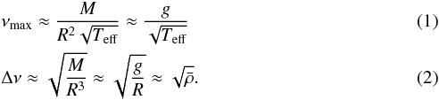 These scaling relations are used with respect to solar values. We discuss previous investigations of possible inaccuracies or biases in the scaling relations in more detail, followed by a discussion of the solar reference values.
2.1. νmax scaling relation
The scaling relation for νmax (Eq. (1)) is an empirical relation in which νmax scales with the acoustic cut-off frequency (Brown et al. 1991). The validity of this relation has recently been tested theoretically by Belkacem et al. (2011). They find a relation between the frequency at which the mode lifetime forms a plateau (i.e., νmax), and the acoustic cut-off frequency, with a coefficient that depends on the ratio of the Mach number of the exciting turbulence to the third power to the mixing-length parameter. So far the relation between this plateau and νmax has not been justified theoretically. Nevertheless, this result is an important step towards understanding the underlying physics of the νmax scaling relation. At this stage, the practical difficulties estimating the Mach number in the upper stellar envelopes implies that it is difficult to use these ideas to predict possible biases or inaccuracies in the νmax scaling relation.
2.2. Δν scaling relation
From stellar models, White et al. (2011) show that proportionality between the mean density of the star and the large frequency separation squared (Eq. (2)) shows discrepancies of a few percent for stars evolving from the zero age main sequence (ZAMS) up towards the tip of the red giant branch, with a clear correlation with the effective temperature. The amount of the discrepancy can be as large as 2–3% in either a positive or negative sense depending on the temperature of the star. we investigate here is expected to be a bias similar for global parameters from different methods. It is important to understand whether this correction has a significant effect on the determined values of log (g). We tested this and find that the difference between the results with and without these corrections are not significant (see Sect. 5).
Miglio et al. (2012) have investigated the accuracy of the Δν scaling relation for stars on the red-giant branch (RGB) and in the red clump (RC). They find that the sound speed in the RC model of 1.2 M⊙ is on average higher (at a given fractional radius) than that of the RGB model of the same mass and radius, the main reason being the different temperature profile in the two models. Miglio et al. (2012) note that while the largest contribution to the overall difference originates in the deep interior, near-surface regions (r/R ≳ 0.9) also contribute (by 0.8 percent) to the total 3.5 percent difference in total acoustic radius. This percentage is expected to be mass-dependent and to be higher for low-mass stars, which have significantly different internal structure when ascending the RGB compared to when they are in the core He-burning phase. Miglio et al. (2012) did not derive an accurate theoretical correction of the Δν scaling. The suggested change in the Δν scaling relation is, however, close to the one mentioned by White et al. (2011). Because these changes caused a difference in log (g) well below the uncertainties (see Sect. 5), we do not expect a significant impact on the determined log (g) values from the effect mentioned by Miglio et al. (2012), so we do not investigate this further.
Mosser et al. (2013) state that using the value of the large separation around νmax is only a proxy and that the solar reference value in Eq. (2) should be the asymptotic value. We comment further on this in Sect. 2.3.
2.3. Solar reference values
The scaling relations (Eqs. (1) and (2)) are expressed in terms of the relevant solar reference values. Changing the solar reference value for νmax will induce an offset in log (g) proportional to the logarithm of their ratio. This means that, for example, changing the solar reference for νmax from 3050 μHz (e.g. Kjeldsen & Bedding 1995) to 3120 μHz (e.g. Kallinger et al. 2010) will induce a change in log (g) of about 0.02 dex (cgs), which is significant.
Additionally, Mosser et al. (2013) argue that using the observed solar values in the scaling relations (Eqs. (1) and (2)) is not actually correct and that this would introduce biases of a few percent in Δν. They suggest that one should be using the asymptotic value of Δν valid at high-order modes (higher order than the observed modes). Using this paradigm the reference values derived become Δν = 138.8 μHz and νmax = 3106 μHz (Mosser et al. 2013). These are valid for stars with masses below 1.3 M⊙ and effective temperatures between 6500 and 5000 K reflecting the range of stars for which the scaling relations are most reliable (White et al. 2011).
In this work we did not implement the asymptotic solar reference values. Firstly, as stated by the authors the change in Δν of the observed star and the reference Δν are similar and the net effect of these changes on the derived log (g) is small. Even if this implies a few percent change in Δν, the tests with the White et al. (2011) corrections show that the effect on log (g) is negligible. Secondly, no asymptotic solar reference values are available in the temperature range of the red giants.
3. Determination of surface gravity
3.1. Data
We perform this study for the same sample of stars as used by Hekker et al. (2012), for which there was agreement in the global oscillation parameters obtained by the different methods and for which there are results from three methods (see Sect. 3.2). This resulted in a list of 707 red giants. For a subset of these stars we know their evolutionary phases determined from period spacings of mixed modes (Beck et al. 2011; Bedding et al. 2011; Mosser et al. 2011a) and the phase shift of the central radial mode (Kallinger et al. 2012). Their locations in an H-R diagram are shown in Fig. 1. For these stars we use Kepler timeseries corrected for instrumental effects in the way described by García et al. (2011). For the effective temperatures we use the SDSS temperatures calibrated with the infrared flux method (Pinsonneault et al. 2012). The evolutionary phases are determined from different methods, i.e., period spacings of mixed modes (Bedding et al. 2011; Mosser et al. 2011a, 2012b; Stello et al. 2013) and phase shift of the central radial mode (Kallinger et al. 2012).
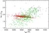 |
Fig. 1 Hertzsprung-Russell diagram for stars used in this survey using SDSS temperatures calibrated with the infrared flux method (Pinsonneault et al. 2012) and luminosities computed using the asteroseismic radii computed using the OCT method and BaSTI models (see Sect. 3). Red-clump stars, red-giant branch stars and stars of unknown evolutionary phase are shown in red, green, and black, respectively. The symbol sizes are proportional to the derived asteroseismic masses of the targets. |
Figure 1 has a few characteristics that are noteworthy. First of all this figure emphasizes again that we need asteroseismology to distinguish between hydrogen-shell burning (RGB) and helium-core burning (RC) stars, because both types of stars can occupy the same location in an H-R diagram. Secondly, Fig. 1 shows that for stars above the RC, it is much more difficult to determine the period spacings and thus the evolutionary phase. This is in part due the fact that stars high on the RGB oscillate with longer periods and at these lower frequencies the frequency resolution of the data becomes a limiting factor. Additionally the coupling between the p- and g- mode cavity becomes weaker which reduces the number of mixed modes visible at the surface; however, this is not true for stars just above the RC. The reason for the non-detections of the period spacings for these stars is at least partly rotation (Mosser et al. 2012b).
3.2. Extraction of global oscillation parameters
The global seismic parameters Δν and νmax are derived from the data using three different methods:
-
CAN: Δν is obtained from fitting a sequence of Lorentzian profiles spanning three radial orders to the background corrected Fourier power spectrum. This method only considers the central part of the oscillation frequency range and is referred to as a “local” method. The parameter νmax is defined as the centroid of a Gaussian profile fitted on top of two Harvey-like background components in the Fourier power spectrum (Kallinger et al. 2010, 2012). In this determination of νmax the full frequency range is considered in the fitting, so this is referred to as a “global” approach.
-
COR: Δν is obtained from the envelope autocorrelation function (EACF) of the time series (Mosser & Appourchaux 2009) and updated using the universal pattern (UP, Mosser et al. 2011b). This method takes a relatively wide frequency range into account and is also a global method. The value of νmax is obtained as the centre of a Gaussian fit on top of a background computed as the mean slope in log-log (Mosser et al. 2012a). The background is computed based on relatively narrow frequency intervals bracketing the frequencies at which oscillations have been detected. Therefore, for νmax this is referred to as a local approach.
-
OCT: Δν is obtained from the power spectrum of the power spectrum. This method is in between the COR and CAN methods in the sense that it probes a narrower frequency range than COR, but a wider frequency range than CAN. The value of νmax is determined as the centroid of a Gaussian fit through a smoothed Fourier power spectrum on top of a background that was first computed with one Harvey-like background component and subsequently improved using the mean slope in log-log (Hekker et al. 2010a). Because the full frequency range was taken into account in the background fitting for the initial step and in the second step an optimization using relatively narrow frequency intervals bracketing the frequencies at which oscillations have been detected. This νmax is referred to as a “semi-global” approach.
The differences in the resulting values for Δν from the local and global approaches are significant and allow one to distinguish between red-giant branch stars and red-clump stars (Kallinger et al. 2012; Hekker et al. 2012). The differences in νmax seem more homogeneously distributed.
3.3. Surface gravity
The surface gravity can be computed from the scaling relations (Eqs. (1) and (2)) directly or by using grid-based modelling, which is performed by two independent implementations based on the recipe described by Basu et al. (2010). One implementation uses BaSTI models (Cassisi et al. 2006). The other implementation uses YY isochrones (Demarque et al. 2004), models constructed with the Dartmouth stellar evolution code (Dotter et al. 2007) and the model grid of Marigo et al. (2008).
Gai et al. (2011) have already shown that asteroseismic log (g) is largely model independent. This is confirmed in this study, and the results of the different grids are primarily used to validate the results.
3.4. Solar reference values
The solar values of νmax and Δν are used in both the direct method and in the grid-based modelling. We analysed one year of solar data from the green SPM channel of SOHO/VIRGO (Frohlich et al. 1997) with the three methods CAN, COR, and OCT and find the following:
-
CAN: Δν = 134.88 ± 0.04 μHz; νmax = 3120 ± 5 μHz (Kallinger et al. 2010);
-
COR: Δν = 134.9 ± 0.1 μHz; νmax = 3060 ± 10 μHz. Note that only the EACF method can be applied to the solar data;
-
OCT: Δν = 135.03 ± 0.07 μHz and νmax = 3140 ± 13 μHz.
The solar reference values for νmax obtained with the different methods are not consistent with each other within 1-sigma. For Δν the CAN and COR values are consistent with each other within one-sigma, while this is not the case for the OCT value. The various numbers are formally different but still well within any three-sigma limit. We expect the main sources for the different solar values for Δν and νmax obtained with the different methods to lie in the use of different definitions in determining the values. The computation of a mean value of Δν is sensitive to the frequency range that is considered. The observational definition of νmax is also different in different methods and depends on whether smoothing is applied or not. Furthermore, νmax is sensitive to the fitted background.
We have investigated the impact of these differences, that is, we analysed the data for log (g) using Δν and νmax from CAN, COR, and OCT with method specific solar reference values obtained from VIRGO data, as well as with a so-called intermediate canonical solar reference value: Δν = 135.1 μHz and νmax = 3090 μHz (Huber et al. 2011, 2013). The results of these tests are shown and discussed in Sects. 5 and 6.
4. Tests applied
For testing the impact on log (g) of differences in Δν and νmax we computed surface gravities using the global seismic parameters from CAN, COR, and OCT using the method-specific solar reference value from VIRGO data or the canonical solar value. We also computed values for the surface gravities with and without the correction to the Δν scaling relation proposed by White et al. (2011). This results in the following tests:
-
Test 1: grid-based modelling using the original scaling relations and the canonical solar reference values;
-
Test 2: grid-based modelling using the original scaling relations and method-specific solar reference values;
-
Test 3: grid-based modelling using the scaling relation for Δν adapted as suggested by White et al. (2011) and canonical solar reference values;
-
Test 4: grid-based modelling using the scaling relation for Δν adapted as suggested by White et al. (2011) and the method-specific solar reference values.
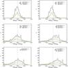 |
Fig. 2 Histograms of the difference in log (g) obtained with different methods (top row: OCT-CAN; centre row: COR-CAN; bottom row: COR-OCT) and with different solar reference values (left: canonical solar reference values (test 1); right: method specific solar reference values (test 2)). The black solid line indicates the complete sample, the red-dashed line the red-clump stars and the green-dashed-dotted line stars on the red-giant branch. We did not know the evolutionary phase for all the stars. The dotted lines show Gaussian fits to the distributions. The central value and formal 1σ uncertainties are given in the legend of each panel. A Gaussian fit through the RC data in the lower left panel did not properly represent the distribution so it is omitted. The vertical dashed line indicates zero difference. |
Summary of ensemble systematics and uncertainties for log (g) using νmax and Δν obtained with different methods using the same canonical solar reference values (test 1).
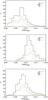 |
Fig. 3 Distribution of the uncertainties in log (g) using global oscillations from CAN, COR, and OCT (top to bottom) and canonical solar reference values (test 1). The colour-coding is the same as in Fig. 2. |
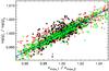 |
Fig. 4 Ratios of νmax values from different methods vs. log (g) values derived from these respective νmax values. Ratios of different methods are indicated with different colours: black asterisks indicate CAN/OCT; red crosses indicate CAN/COR; green diamonds indicate OCT/COR. The blue solid line is a fit to all results. |
5. Results
5.1. Direct method
Given Eq. (1), we expect a ~0.4% change in log (g) upon a 1% change in νmax. In the next section we explore the sensitivity of grid-based search methods to changes in both Δν and νmax in the range 5 μHz < νmax < 250 μHz.
5.2. Grid modelling
The results of the different experiments as listed in the previous section are shown in Fig. 2. These are histograms of the differences in obtained log (g) values from grid-based modelling using global oscillation parameters derived using the different data analysis methods CAN, COR, and OCT.
The two columns in Fig. 2 show the results of tests 1 and 2 (see Sect. 4). Each row shows the difference between two of the methods. The distributions in the top panels are higher and narrower compared to the distributions in the middle and bottom row. This shows that the CAN and OCT approaches to the determination in νmax give more similar results in log (g) than the approach adopted by COR. See also Table 1 for the relative systematics of the results.
Going from the left- to the right-hand panels of Fig. 2, the canonical solar reference values (test 1) are changed to the method-specific solar reference values obtained from the analysis of VIRGO data (test 2). It is clear that using different solar reference values introduces a bias in the determinations of log (g). The shifts are consistent with the difference in solar reference values used for νmax. In other words, it follows from the scaling relation that Δlog (g) ∝ log (νmax ⊙ ,1/νmax ⊙ ,2). However, it is well known that different methods produce different outputs for the solar values. Therefore, we had expected that the difference in log (g) would be reduced when using the solar reference values and observed stellar values obtained using a given method (test 2, right column). Evidently, this is not the case. The difference in log (g) values is significantly smaller when the same solar reference values are used (test 1, left column). This essentially shows that the relative difference in obtained solar values with the different methods is significantly more than the relative difference in νmax obtained for red giants between each of the methods.
The left-hand histograms in Fig. 2 (test 1) also show that there are always offsets between the RGB and RC distributions. We find that for RGB stars the lowest log (g) is obtained with global oscillation parameters from OCT, and slightly higher values from COR and CAN. For RC stars the distributions are less well defined, making it difficult to be quantitative.
The uncertainties in log (g) (Fig. 3 and Table 1) show distributions that peak at around 0.01 dex. These distributions are similar for all four tests. In general it seems as if the uncertainty distribution of the RGB stars peaks at slightly higher uncertainties than for RC stars. For CAN and OCT the uncertainties in the RC stars show a wider, flatter distribution compared to the uncertainties of COR indicating that the COR uncertainties are more consistent, albeit slightly higher, than for the other methods.
As indicated earlier, we also investigate the correction to the Δν scaling relation by White et al. (2011). The difference between the results with and without the correction for a specific method are shown in Fig. 5. This figure shows that indeed the impact of the 2–3% correction in Δν on log (g) is of the order of 0.001, which is well within the uncertainties of the results (see Fig. 3). This is consistent with what we expect from Eq. (1). We note that a change of a few percent in Δν will have a significant effect on the determination of the mass and radius.
To investigate the improvement in accuracy of log (g) obtained from grid-based search methods compared to asteroseismic scaling relations, we show the ratio of νmax obtained with different methods vs the ratio of log (g) based on the respective νmax values (see Fig. 4). We fit a straight line through the ratios and find a slope of 0.171 ± 0.001. This uncertainty indicates a one-sigma uncertainty estimate of the slope. This indicates a change of 0.171% in log (g) upon a change of 1% in νmax. This is a significantly lower sensitivity than ~0.4% change in log (g) upon a 1% change in νmax expected from scaling relations. We attribute this to the inclusion of additional constraints in grid-based search methods.
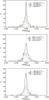 |
Fig. 5 Histograms of the difference in log (g) obtained using grid-based modelling with the same method, but with and without the correction in the Δν scaling relation (White et al. 2011). From top to bottom: CAN, COR, and OCT. The central values of the distributions and formal 1σ uncertainties are given in the legend of each panel. The vertical dashed line indicates zero. The colour-coding is the same as in Fig. 2. Note that the horizontal scale has been expanded. |
6. Discussion
There is a significant spread in the derived log (g) values between COR and either CAN or OCT. This wide spread indicates not that the COR values are systematically higher or lower than CAN/OCT, but that they show a larger scatter compared to CAN/OCT results. We can understand this as indicating that a less accurate log (g) is derived when using COR parameters. This could be because both CAN and OCT use a more global approach in which they include more prior information to fit the background, while COR uses only a local mean slope in log-log without prior information. Reliable determination of νmax depends on a good determination of the granulation background spectrum. It is possible to argue that the fully global approach of CAN provides the best possible determination of the background, hence of νmax. Ideally one would verify this by computing log (g) from a Fourier power spectrum obtained from a model for which we know log (g). Currently the uncertainties in such an approach are too large to have any added value for this analysis.
There are large biases when using a solar reference value computed with the same method. We understand these biases as a sign that the current methods are optimised for analysis of frequencies in the red giant regime and not in the solar regime, which leads to relatively large scatter in the solar values compared to the scatter in values determined for red giants. The higher amplitudes of the modes, the lower number of orders, as well as the narrow frequency range of the oscillations are likely to improve the consistency between the derived global parameters from different methods.
One might argue that the frequency regime of the solar reference is too different from that of the red giants. When it comes to red giants, we might therefore consider a “platinum standard”, i.e., a reference star that is another red giant. This needs to be a star with extremely well-constrained properties obtained from independent methods. A detached eclipsing binary such as analysed by Hekker et al. (2010b) could be a suggestion. For this star there is an orbital solution, and the mass and radius have been determined accurately (Frandsen, priv. comm.). However, this star has a complicate oscillation pattern, and the evolutionary phase has not been determined yet.
Our suggestion is to derive the most accurate value for log (g) using oscillation parameters from CAN or OCT with canonical solar reference values. The log (g) values from CAN parameters have slightly smaller uncertainties. The drawback of this method that it is relatively time consuming and is not fully automated. The log (g) values from OCT parameters have slightly higher uncertainties. Nevertheless, this method shows only small biases in log (g), which are well within the uncertainties, and it is faster than CAN and fully automated. Therefore, we suggest using oscillation parameters from OCT to obtain a homogeneous analysis. It remains, however, essential that a selection of methods is applied to validate the results of the chosen method.
We note that there are biases in the distributions between red-clump and red-giant branch stars. These could be due to the differences arising from a “local” or “global” approach. Kallinger et al. (2012) and Hekker et al. (2012) have shown that at least for Δν it is possible to distinguish between red-clump and red-giant branch stars by the difference in results from the “local” or “global” method. Hekker et al. (2012) did not find any evidence that νmax could be used to distinguish between red-clump and red-giant branch stars. However, the results presented here could indicate that it is possible to identify the evolutionary phase of the star from the determination of a “local” or “global” νmax.
In this work we have focussed on determining log (g), for which small changes in Δν are insignificant. We recognize, however, that a change of a few percent in Δν will have a significant effect on the determination of the mass and radius of the star. Using the scaling relations (Eqs. (1) and (2)), it is straightforward to derive that a 5% uncertainty in νmax and 2% uncertainty in Δν lead to a ~10% uncertainty in stellar mass and a ~6% uncertainty in stellar radius. This is significantly higher than the ~2% uncertainty in log (g) upon a 5% uncertainty in νmax.
7. Conclusions
For grid-based modelling we compared the log (g) values obtained from the seismic parameters derived with the CAN, COR, and OCT methods using a grid of BaSTI models. We can draw the following conclusions.
-
The log (g) values from oscillation parameters from the CAN and OCT method are more similar and precise than the results from COR;
-
The use of the same canonical solar reference values reduces the biases in log (g) compared to using method-specific solar reference values (this is at least true for red giants analysed here);
-
There are small biases between the results for red-clump and red-giant branch stars;
-
The uncertainties in log (g) are of the order of 0.01 dex (cgs);
-
The biases due to different methods are within the uncertainties when using the same canonical solar reference values;
-
The correction in the Δν scaling equation of 2–3%, as proposed by White et al. (2011), does not influence the determination of log (g) significantly;
-
Grid-based search methods show that log (g) values have a lower sensitivity to small changes in νmax than is apparent from the direct scaling relations.
Acknowledgments
We thank R. A. García (CEA) for all the time and efforts he has put into the correction of the raw Kepler data to make them suitable for the analyses presented in this paper. S.H. acknowledges financial support from the Netherlands Organisation for Scientific Research (NWO). Y.E. and W.J.C. acknowledge support from STFC (The Science and Technology Facilities Council, UK). S.B. acknowledges NSF grant AST-1105930 and NASA grant 495 NNX13AE70G. T.K. acknowledges financial support from the Austrian Science Fund (FWF P23608). This work made use of BaSTI web tools. SOHO is a mission of international collaboration between ESA and NASA
References
- Basu, S., Chaplin, W. J., & Elsworth, Y. 2010, ApJ, 710, 1596 [NASA ADS] [CrossRef] [Google Scholar]
- Beck, P. G., Bedding, T. R., Mosser, B., et al. 2011, Science, 332, 205 [NASA ADS] [CrossRef] [PubMed] [Google Scholar]
- Bedding, T. R., Mosser, B., Huber, D., et al. 2011, Nature, 471, 608 [NASA ADS] [CrossRef] [PubMed] [Google Scholar]
- Belkacem, K., Goupil, M. J., Dupret, M. A., et al. 2011, A&A, 530, A142 [NASA ADS] [CrossRef] [EDP Sciences] [Google Scholar]
- Brown, T. M., Gilliland, R. L., Noyes, R. W., & Ramsey, L. W. 1991, ApJ, 368, 599 [NASA ADS] [CrossRef] [Google Scholar]
- Cassisi, S., Pietrinferni, A., Salaris, M., et al. 2006, Mem. Soc. Astron. It., 77, 71 [Google Scholar]
- Creevey, O. L., & Thévenin, F. 2012, in SF2A-2012: Proc. Annual meeting of the French Society of Astronomy and Astrophysics, eds. S. Boissier, P. de Laverny, N. Nardetto, R. Samadi, D. Valls-Gabaud, & H. Wozniak, 189 [Google Scholar]
- Creevey, O. L., Thévenin, F., Basu, S., et al. 2013, MNRAS, 431, 2419 [NASA ADS] [CrossRef] [Google Scholar]
- Demarque, P., Woo, J.-H., Kim, Y.-C., & Yi, S. K. 2004, ApJS, 155, 667 [NASA ADS] [CrossRef] [Google Scholar]
- Dotter, A., Chaboyer, B., Jevremović, D., et al. 2007, AJ, 134, 376 [NASA ADS] [CrossRef] [Google Scholar]
- Frohlich, C., Andersen, B. N., Appourchaux, T., et al. 1997, Sol. Phys., 170, 1 [NASA ADS] [CrossRef] [Google Scholar]
- Gai, N., Basu, S., Chaplin, W. J., & Elsworth, Y. 2011, ApJ, 730, 63 [NASA ADS] [CrossRef] [Google Scholar]
- García, R. A., Hekker, S., Stello, D., et al. 2011, MNRAS, 414, L6 [NASA ADS] [CrossRef] [Google Scholar]
- Hekker, S., & Meléndez, J. 2007, A&A, 475, 1003 [NASA ADS] [CrossRef] [EDP Sciences] [Google Scholar]
- Hekker, S., Broomhall, A.-M., Chaplin, W. J., et al. 2010a, MNRAS, 402, 2049 [NASA ADS] [CrossRef] [Google Scholar]
- Hekker, S., Debosscher, J., Huber, D., et al. 2010b, ApJ, 713, L187 [NASA ADS] [CrossRef] [Google Scholar]
- Hekker, S., Elsworth, Y., De Ridder, J., et al. 2011, A&A, 525, A131 [NASA ADS] [CrossRef] [EDP Sciences] [Google Scholar]
- Hekker, S., Elsworth, Y., Mosser, B., et al. 2012, A&A, 544, A90 [NASA ADS] [CrossRef] [EDP Sciences] [Google Scholar]
- Huber, D., Bedding, T. R., Stello, D., et al. 2011, ApJ, 743, 143 [NASA ADS] [CrossRef] [Google Scholar]
- Huber, D., Chaplin, W. J., Christensen-Dalsgaard, J., et al. 2013, ApJ, 767, 127 [NASA ADS] [CrossRef] [Google Scholar]
- Kallinger, T., Mosser, B., Hekker, S., et al. 2010, A&A, 522, A1 [NASA ADS] [CrossRef] [EDP Sciences] [Google Scholar]
- Kallinger, T., Hekker, S., Mosser, B., et al. 2012, A&A, 541, A51 [NASA ADS] [CrossRef] [EDP Sciences] [Google Scholar]
- Kjeldsen, H., & Bedding, T. R. 1995, A&A, 293, 87 [NASA ADS] [Google Scholar]
- Marigo, P., Girardi, L., Bressan, A., et al. 2008, A&A, 482, 883 [NASA ADS] [CrossRef] [EDP Sciences] [Google Scholar]
- Miglio, A., Brogaard, K., Stello, D., et al. 2012, MNRAS, 419, 2077 [NASA ADS] [CrossRef] [Google Scholar]
- Morel, T., & Miglio, A. 2012, MNRAS, 419, L34 [NASA ADS] [CrossRef] [Google Scholar]
- Mosser, B., & Appourchaux, T. 2009, A&A, 508, 877 [NASA ADS] [CrossRef] [EDP Sciences] [Google Scholar]
- Mosser, B., Barban, C., Montalbán, J., et al. 2011a, A&A, 532, A86 [NASA ADS] [CrossRef] [EDP Sciences] [Google Scholar]
- Mosser, B., Belkacem, K., Goupil, M. J., et al. 2011b, A&A, 525, L9 [NASA ADS] [CrossRef] [EDP Sciences] [Google Scholar]
- Mosser, B., Elsworth, Y., Hekker, S., et al. 2012a, A&A, 537, A30 [NASA ADS] [CrossRef] [EDP Sciences] [Google Scholar]
- Mosser, B., Goupil, M. J., Belkacem, K., et al. 2012b, A&A, 540, A143 [NASA ADS] [CrossRef] [EDP Sciences] [Google Scholar]
- Mosser, B., Michel, E., Belkacem, K., et al. 2013, A&A, 550, A126 [NASA ADS] [CrossRef] [EDP Sciences] [Google Scholar]
- Pinsonneault, M. H., An, D., Molenda-Żakowicz, J., et al. 2012, ApJS, 199, 30 [NASA ADS] [CrossRef] [Google Scholar]
- Stello, D., Bruntt, H., Preston, H., & Buzasi, D. 2008, ApJ, 674, L53 [NASA ADS] [CrossRef] [Google Scholar]
- Stello, D., Chaplin, W. J., Basu, S., Elsworth, Y., & Bedding, T. R. 2009, MNRAS, 400, L80 [NASA ADS] [CrossRef] [Google Scholar]
- Stello, D., Huber, D., Bedding, T. R., et al. 2013, ApJ, 765, L41 [NASA ADS] [CrossRef] [Google Scholar]
- Thygesen, A. O., Frandsen, S., Bruntt, H., et al. 2012, A&A, 543, A160 [NASA ADS] [CrossRef] [EDP Sciences] [Google Scholar]
- White, T. R., Bedding, T. R., Stello, D., et al. 2011, ApJ, 743, 161 [NASA ADS] [CrossRef] [Google Scholar]
All Tables
Summary of ensemble systematics and uncertainties for log (g) using νmax and Δν obtained with different methods using the same canonical solar reference values (test 1).
All Figures
|
Fig. 1 Hertzsprung-Russell diagram for stars used in this survey using SDSS temperatures calibrated with the infrared flux method (Pinsonneault et al. 2012) and luminosities computed using the asteroseismic radii computed using the OCT method and BaSTI models (see Sect. 3). Red-clump stars, red-giant branch stars and stars of unknown evolutionary phase are shown in red, green, and black, respectively. The symbol sizes are proportional to the derived asteroseismic masses of the targets. |
| In the text | |
|
Fig. 2 Histograms of the difference in log (g) obtained with different methods (top row: OCT-CAN; centre row: COR-CAN; bottom row: COR-OCT) and with different solar reference values (left: canonical solar reference values (test 1); right: method specific solar reference values (test 2)). The black solid line indicates the complete sample, the red-dashed line the red-clump stars and the green-dashed-dotted line stars on the red-giant branch. We did not know the evolutionary phase for all the stars. The dotted lines show Gaussian fits to the distributions. The central value and formal 1σ uncertainties are given in the legend of each panel. A Gaussian fit through the RC data in the lower left panel did not properly represent the distribution so it is omitted. The vertical dashed line indicates zero difference. |
| In the text | |
|
Fig. 3 Distribution of the uncertainties in log (g) using global oscillations from CAN, COR, and OCT (top to bottom) and canonical solar reference values (test 1). The colour-coding is the same as in Fig. 2. |
| In the text | |
|
Fig. 4 Ratios of νmax values from different methods vs. log (g) values derived from these respective νmax values. Ratios of different methods are indicated with different colours: black asterisks indicate CAN/OCT; red crosses indicate CAN/COR; green diamonds indicate OCT/COR. The blue solid line is a fit to all results. |
| In the text | |
|
Fig. 5 Histograms of the difference in log (g) obtained using grid-based modelling with the same method, but with and without the correction in the Δν scaling relation (White et al. 2011). From top to bottom: CAN, COR, and OCT. The central values of the distributions and formal 1σ uncertainties are given in the legend of each panel. The vertical dashed line indicates zero. The colour-coding is the same as in Fig. 2. Note that the horizontal scale has been expanded. |
| In the text | |
Current usage metrics show cumulative count of Article Views (full-text article views including HTML views, PDF and ePub downloads, according to the available data) and Abstracts Views on Vision4Press platform.
Data correspond to usage on the plateform after 2015. The current usage metrics is available 48-96 hours after online publication and is updated daily on week days.
Initial download of the metrics may take a while.