| Issue |
A&A
Volume 556, August 2013
|
|
|---|---|---|
| Article Number | A30 | |
| Number of page(s) | 9 | |
| Section | Stellar structure and evolution | |
| DOI | https://doi.org/10.1051/0004-6361/201321248 | |
| Published online | 19 July 2013 | |
XMM-Newton and Swift observations of XTE J1743-363⋆
1
ISDC Data Centre for Astrophysics, department of Astronomy, University of
Geneva, Chemin d’Écogia
16, 1290
Versoix,
Switzerland
e-mail:
This email address is being protected from spambots. You need JavaScript enabled to view it.
2
INAF, Istituto di Astrofisica Spaziale e Fisica Cosmica –
Palermo, via U. La Malfa
153, 90146
Palermo,
Italy
3
INAF – Osservatorio Astronomico di Brera,
via Bianchi 46, 23807
Merate ( LC), Italy
4
International Space Science Institute (ISSI) Hallerstrasse
6, 3012
Bern,
Switzerland
5
INAF – Osservatorio Astronomico di Roma, via Frascati
33, 00044
Roma,
Italy
Received:
6
February
2013
Accepted:
6
June
2013
Abstract
XTE J1743-363 is a poorly known hard X-ray transient, which displays short and intense flares similar to those observed from supergiant fast X-ray transients. The probable optical counterpart shows spectral properties similar to those of an M8 III giant, thus suggesting that XTE J1743-363 belongs to the class of the symbiotic X-ray binaries class. In this paper we report on the first dedicated monitoring campaign of the source in the soft X-ray range with XMM-Newton and Swift /XRT. These observations confirmed the association of XTE J1743-363 with the previously suggested M8 III giant and the classification of the source as a member of the symbiotic X-ray binaries. In the soft X-ray domain, XTE J1743-363 displays a high absorption (~6 × 1022 cm-2) and variability on time scales of hundreds to few thousand seconds, typical of wind-accreting systems. A relatively faint flare (peak X-ray flux 3 × 10-11 erg/cm2/s) lasting ~4 ks is recorded during the XMM-Newton observation and interpreted in terms of the wind accretion scenario.
Key words: X-rays: binaries / X-rays: individuals: XTE J1743-363
Table 2 is available in electronic for at http://www.aanda.org
© ESO, 2013
1. Introduction
XTE J1743-363 was discovered by Markwardt et al. (1999) during RXTE monitoring observations of the Galactic-center region. At that time, the source was detected undergoing episodes of enhanced X-ray activity, reaching fluxes of 15 mCrab and showing variability with time scales as short as ~1 min. The source was also observed undergoing intense short outbursts with INTEGRAL and was thus classified as a possible supergiant fast X-ray transient (SFXT, see, e.g., Sguera et al. 2006). The brightest outburst from the source observed with INTEGRAL reached about 40 mCrab in the 20–60 keV energy band and lasted ~2.5 h. Before the present work, XTE J1743-363 was not studied with focusing X-ray telescopes in the soft X-ray domain (0.3–12 keV) and the position of the source could be securely measured only with an accuracy of a few arcmin. A possible sub-arcmin localization of the source was proposed by Ratti et al. (2010) using an archival Chandra observation. In those data, about 11 photons were serendipitously recorded from a location in the relatively large INTEGRAL error circle around the position of XTE J1743-363. Based on this, Smith et al. (2012) proposed a probable optical counterpart that displays typical spectral characteristics of an M8III giant, suggesting that XTE J1743-363 could be a new member of the symbiotic X-ray binary (SyXB) class rather than an SFXT (though some uncertainties still prevent a firm conclusion about the precise spectral type of the companion). Smith et al. (2012) also reported a complete re-analysis of all RXTE /PCA data of the source and showed that its X-ray flux has continuously decreased during the past ~13 yrs. Such a behavior was not observed before in an SFXT.
We report in this paper on the first pointed observations of XTE J1743-363 with focusing X-ray instruments. These include a deep pointing with XMM-Newton (total exposure time 42 ks) and a three-month-long monitoring campaign performed with Swift /XRT (total on-source exposure time 79 ks).
2. XMM-Newton data analysis and results
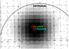 |
Fig. 1 Refined XMM position (1.5′′ at 68% c.l.) of the source reported in the present work is compatible with the Chandra position of the faint source detected by Ratti et al. (0.6′′ at 90% c.l.; 2010) and is suggested to be the quiescent counterpart to XTE J1743-363. We also show the INTEGRAL position (0.7′ at 90% c.l.; Bird et al. 2010) and the Swift /XRT position (2.3′′ at 90% c.l.; see Sect. 3). |
Starting on 2012 February 29 18:31 UT, XMM-Newton observed XTE J1743-363 for about 42 ks. The EPIC-pn was operated in full-frame, the EPIC-MOS1 in small window, and the MOS2 in timing mode. Observation data files (ODFs) were processed to produce calibrated event lists using the standard XMM-Newton Science Analysis System (v. 12.0.1). We used the epproc and emproc tasks to produce cleaned event files from the Epic-pn and MOS cameras, respectively. The Epic-pn and Epic-MOS event files were filtered in the 0.3–12 keV and 0.5–10 keV energy range, respectively. High background time intervals were excluded using standard techniques1. The effective exposure time was 33 ks for the EPIC-pn and 40 ks for the MOS cameras. Lightcurves and spectra of the source and background were extracted by using regions in the same CCD for the MOS and from adjacent CCDs at the same distance to the readout node for the EPIC-pn2. The difference in extraction areas between source and background was accounted for by using the SAS backscale task for the spectra and lccorrr for the lightcurves. All EPIC spectra were rebinned before fitting in order to have at least 15–25 counts per bin (depending on the statistics of each spectrum) and, at the same time, prevent oversampling of the energy resolution by more than a factor of three. Where required, we barycenter-corrected the photon arrival times in the EPIC event files with the barycen tool. Throughout this paper, uncertainties are given at 90% c.l., unless stated otherwise.
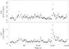 |
Fig. 2 EPIC-pn lightcurve of XTE J1743-363 in the 0.3–3.5 keV (upper panel) and 3.5–12 keV (lower panel) energy band. The start time is 55 986.8017 MJD and the bin time is 200 s. |
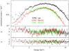 |
Fig. 3 EPIC-pn (black), EPIC-MOS1 (red), and EPIC-MOS2 (green) spectra of XTE J1743-363 extracted by using the entire exposure time available from the XMM-Newton observation. The best fit is obtained here with an absorbed BMC model. The residuals from this fit are shown in the bottom panel. The middle panel shows the residuals from a fit with a simple power-law model. |
The best position of XTE J1743-363 determined by the EPIC-pn and MOS1 is at
αJ2000 = 17h43m01 44 and
δJ2000 = −36°22′23
44 and
δJ2000 = −36°22′23 16, with an
associated uncertainty of 1.5 arcsec. at 68% c.l.3. In
Fig. 2 we show the EPIC-pn background-subtracted source
lightcurve in two energy bands. A flare from the source is observed about 30 ks after the
beginning of the observation. The averaged EPIC-pn, MOS1, and MOS2 spectra of the
observation are shown in Fig. 3. A simultaneous fit to
all spectra4 with a simple absorbed power-law model
gave an absorption column density
NH = (6.1 ± 0.2) × 1022 cm-2, a photon
index Γ = 1.51 ± 0.05, and a poor
16, with an
associated uncertainty of 1.5 arcsec. at 68% c.l.3. In
Fig. 2 we show the EPIC-pn background-subtracted source
lightcurve in two energy bands. A flare from the source is observed about 30 ks after the
beginning of the observation. The averaged EPIC-pn, MOS1, and MOS2 spectra of the
observation are shown in Fig. 3. A simultaneous fit to
all spectra4 with a simple absorbed power-law model
gave an absorption column density
NH = (6.1 ± 0.2) × 1022 cm-2, a photon
index Γ = 1.51 ± 0.05, and a poor  /d.o.f. =
1.34/314. The observed 2–10 keV X-ray flux was 5.7 × 10⁻¹² erg/cm2/s.
In order to improve the fit, we first considered a bulk motion Comptonization (BMC) model,
which accounts for the soft thermal emission from the neutron star and its Comptonization in
a self-consistent way (Titarchuk et al. 1997). We
then tried a model comprising a mekal (i.e., emission from a thin thermal medium)
and a power-law component (see discussion in Bozzo et al.
2010). The BMC model provided a statistically acceptable fit (see Table 1), but only an upper limit could be obtained on the
spectral index parameter α = Γ−1. This is due to the limited energy
coverage of the XMM-Newton spectra (0.3–12 keV). Other spectral models with
similar numbers of free parameters, including a cut-off power-law or a power-law with an
exponential rollover, also provided reasonably good fits to the data. However, these models
gave very low value of the cut-off and exponential rollover energies (~4 keV) and unlikely
negative power-law photon indices (Γ ~ −0.5). We checked a posteriori that different
choices of the energy binning and background extraction region would not affect these
results.
/d.o.f. =
1.34/314. The observed 2–10 keV X-ray flux was 5.7 × 10⁻¹² erg/cm2/s.
In order to improve the fit, we first considered a bulk motion Comptonization (BMC) model,
which accounts for the soft thermal emission from the neutron star and its Comptonization in
a self-consistent way (Titarchuk et al. 1997). We
then tried a model comprising a mekal (i.e., emission from a thin thermal medium)
and a power-law component (see discussion in Bozzo et al.
2010). The BMC model provided a statistically acceptable fit (see Table 1), but only an upper limit could be obtained on the
spectral index parameter α = Γ−1. This is due to the limited energy
coverage of the XMM-Newton spectra (0.3–12 keV). Other spectral models with
similar numbers of free parameters, including a cut-off power-law or a power-law with an
exponential rollover, also provided reasonably good fits to the data. However, these models
gave very low value of the cut-off and exponential rollover energies (~4 keV) and unlikely
negative power-law photon indices (Γ ~ −0.5). We checked a posteriori that different
choices of the energy binning and background extraction region would not affect these
results.
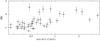 |
Fig. 4 HID of the source realized by using the same lightcurves shown in Fig. 2 adaptively rebinned to a S/N = 9 (see also Fig. 5). |
In order to study possible spectral variations during the observation, we extracted the hardness-intensity diagram (HID) of the source (this was calculated as in our previous papers, see, e.g., Bozzo et al. 2010). From Fig. 4 we noticed that the hardness ratio (HR) could not be easily related to changes of the source overall intensity. To better investigate the behavior of the HR, we rebinned the source lightcurve adaptively in order to have in each bin a signal-to-noise ratio (S/N) of 9. This is shown in Fig. 5.
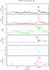 |
Fig. 5 First two panels from the top show the source lightcurves of Fig. 2 rebinned adaptively to a S/N = 9 (based on the lightcurve in the 0.3−3.5 keV energy band). The third panel from the top shows the HR, calculated as the ratio between the source count-rate in the 3.5–12 keV vs. count-rate in the 0.3–3.5 keV energy band. The other three panels show the absorption column density (NH), the power-law photon index (Γ), and the observed flux (units of 10-11 erg/cm2/s) in different time intervals as revealed from our time-resolved spectral analysis (see text for details). |
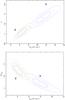 |
Fig. 6 Contours plot (68%, 90%, and 99% c.l.) obtained from the fit to the spectra “b” and “d” with the ph*pl and ph*BMC models (see Fig. 5 and Table 1). |
The complex behavior of the source HR is especially puzzling shortly before until after the bright flare occurring at t ~ 30 ks from the beginning of the observation. In particular, it is evident that the HR significantly increases about 3 ks before the peak of the flare, displays a sudden drop of few hundred seconds immediately after the peak, and then decreases back to the value of the first part of the observation (showing similar but less pronounced variations). We investigated the origin of this variability by dividing the total observation into six time intervals (see Fig. 5) and performing a time-resolved spectral analysis. The EPIC-pn and EPIC-MOS spectra extracted during the same time intervals were fit together to increase the statistics and thus reduce the uncertainties in the fit parameters. Given the shorter exposure times and lower statistics with respect to the spectrum of the entire observation, all time-resolved spectra could be well fit by using a simple power-law model (the only exception being the spectrum “a”, which has the longest exposure time). For consistency with the results obtained from the total spectrum, we also fit the time resolved spectra with the BMC model (we fixed in most cases the value of log (A) and α as these parameters could not be constrained). The results are given in Table 1 and shown in Fig. 5. The fits to the time-resolved spectra with all models suggest there was a significant change in the spectral parameters during the bright flare. The largest variation occurs between the time intervals “b” and “d”. To demonstrate that these changes are not model dependent, we also show in Fig. 6 the contour plots of the spectral parameters of the absorbed BMC and the power-law model, which displayed a significant change during these intervals. We note that the variation of the NH revealed from the fit with a simple absorbed power-law model is fully consistent with the ph*(mkl+pl) interpretation of the X-ray spectrum. During the time passed from the “b” to the “d” time intervals (≲1.5 ks) we would not expect significant changes in the mekal component, as the latter should not vary on timescales shorter than Rmekal/c ~ 2.3 ks (here c is the speed of light and Rmekal > 1013 cm, as estimated in Sect. 4). We verified that the addition of a mekal component with temperature and normalization fixed to the values determined from the total spectrum to the time-resolved spectra would not significantly affect the results presented in Fig. 6.
The results in Figs. 5 and 6 suggest that the absorption column density in the direction of the
source rose up about 3 ks before the onset of the flare, dropped close to the peak of the
event (when the source reached the highest X-ray flux), and then rose again during the
initial decay of the flare. Correspondingly, we observed a flattening of the power-law
photon index (in the fit with the model ph*pl) or an increase in the temperature of the seed
thermal photons in the fit with the ph*BMC model. The interpretation of these results is
discussed in Sect. 4. We note that fixing the same
value of the absorption column density measured for spectrum “d” in the fit to the spectrum
“b” would give unacceptable results in both cases of the ph*pl and ph*BMC models
(/d.o.f. =
1.41/70 and 1.37/70, respectively). The same conclusion applies if the absorption column
density measured for spectrum “b” is used and fixed in the fit to the spectrum “d”. In this
case we obtained for the ph*pl and ph*BMC models /d.o.f. =
1.30/91 and 1.23/91, respectively.
The source and background EPIC MOS and pn event lists were used to carry out an in-depth search for coherent signals after barycenter correction. We applied the power-spectrum search algorithm developed by Israel & Stella (1996) to the lists of barycentered photon arrival times. This method is optimized to search for periodicities in “colored” power spectrum components and provides upper limits if no signal is detected. Due to the different sampling times of the three EPIC cameras we decided to carry out the search in three different ways: (i) by using all the event lists and a binning time of 0.3 s, (ii) by combining the MOS2 and pn event lists with binning time of 73.4 ms (keeping the original Fourier resolution); and (iii) by using only the MOS2 event list with a binning time of 1.75 ms (thus maximizing the Nyquist frequency). No significant signal was found. We show in Fig. 7 the derived 3σ upper limits to the pulsed fraction as a function of the pulse frequency.
3. Swift data analysis and results
The Swift X-ray telescope (XRT, Burrows et al. 2005) data data were obtained as a target of opportunity (ToO) monitoring campaign. The ToO started on 2012 April 19 with 1 ks per day until July 20; then 1 ks observations were carried out every other day. The campaign lasted 115 days, with 82 observations for a total on-source exposure of 79 ks. We also considered the archival Swift observation 00037884001 from 2010 February (see Table 2 for details).
The XRT data were processed with standard procedures (xrtpipeline v0.12.6), and
filtering and screening criteria were applied by using ftools in the heasoft
package (v.6.12). Given the low count rate of the source throughout the monitoring
campaign, we only considered photon-counting (PC) mode data, and selected event grades 0–12
(Burrows et al. 2005). We used the latest spectral
redistribution matrices in CALDB (20120713). The best source position determined with XRT is
at
αJ2000 = 17h43m0131 and
δJ2000 = −36°22′214, with an
associated uncertainty of 2.3′′ at 90% c.l.5.
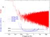 |
Fig. 7 In the upper part of the plot we show the power spectrum produced using the MOS2 event list as an example. In the bottom part of the plot we show the curves representing the upper limits to the non-detection of pulsations calculated according to Israel & Stella (1996). The solid, dashed and dotted lines correspond to the different sampling times and event list combinations discussed in the text. The two horizontal dashed lines represent the 20% and 30% upper limit levels on the pulsed fraction upper limits as a function of the frequency. The most stringent upper limits we could provide are at 20–30% for frequencies in the range 0.005–200 Hz. |
 |
Fig. 8 Long-term monitoring of XTE J1743-363 performed with Swift /XRT (the campaign started about 50 days after the XMM-Newton observation). The count-rate is given in the 0.3–10 keV energy range. Assuming the source averaged spectral properties reported in Sect. 3, a count-rate of 0.01 cts/s corresponds to about 1.2 × 10⁻¹² erg/cm2/s. Downward arrows correspond to 3σ upperlimits on the source count-rate. |
The 0.3–10 keV XRT background-subtracted lightcurve was created at a 1 day resolution and shown in Fig. 8. All count-rate measurements have been corrected for point spread function (PSF) losses and vignetting. The source could not be detected in all observations. In order to preserve a good sampling in time for the source count-rate, we stacked together close-by observations in which a detection of the source could not be obtained after a few days of integration (~2–3). For all isolated non-detections, we indicated in the figure the corresponding 3σ upperlimits on the source count-rate with downward arrows. We did not include in Fig. 8 the observation 00037884001. At the epoch of this observation, XRT did not detect the source and we derived a 90% c.l. upper limit on its X-ray flux of 8 × 10-13 erg/cm2/s (2–10 keV not corrected for absorption). This is the only observation in the soft X-ray domain that overlaps with previously reported RXTE data (see Sect. 4).
For our spectral analysis, we extracted the mean spectrum in the same regions as those
adopted for the light curves; ancillary response files were generated with xrtmkarf
to account for different extraction regions, vignetting, and PSF corrections. The data
were rebinned with a minimum of 20 counts per energy bin and fit in the 0.3–10 keV energy
range. The XRT spectrum (see Fig. 9) could be well fit
(/d.o.f. =
0.90/56) with a simple absorbed power-law model. We obtained
NH = (5.6 ± 0.9) × 1022 cm-2 and
Γ = 1.6 ± 0.3, which is in reasonably good agreement with the average results obtained from
XMM-Newton (Sect. 2). The averaged
observed 2–10 keV X-ray flux was 2.0 × 10⁻¹² erg/cm2/s. For comparison
with results in Sect. 2 we also fit the XRT spectrum
with the ph*BMC model (/d.o.f. =
0.65/56). In this case we obtained  cm-2,
kT = 1.1 ± 0.2 keV, and
NBMC = (2.8 ± 0.3) × 10-5. As XRT recorded a total
of only 1244 counts from the source, we did not attempt a time-resolved spectral analysis of
the XRT data.
cm-2,
kT = 1.1 ± 0.2 keV, and
NBMC = (2.8 ± 0.3) × 10-5. As XRT recorded a total
of only 1244 counts from the source, we did not attempt a time-resolved spectral analysis of
the XRT data.
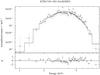 |
Fig. 9 Swift /XRT spectrum extracted by summing up all data in Table 2. The best fit is obtained with a simple absorbed power-law model (see text for details). The residuals from this fit are shown in the bottom panel. |
4. Discussion and conclusions
In this paper, we reported for the first time an in-depth monitoring of XTE J1743-363 in the soft X-ray domain (0.3–12 keV). The position of the source determined from these data at a few arcsec accuracy is compatible with that suggested previously by Ratti et al. (2010), thus confirming the association of XTE J1743-363 with the M8III giant star identified by Smith et al. (2012) and the classification of the source as a SyXBs.
In the XMM-Newton data, the source displayed variability on timescales of
a few hundred to a few thousands of seconds. A relatively bright flare occurred about 30 ks
after the beginning of the observation and lasted for a few ks. Such behavior is reminiscent
of what is often observed in neutron star (NS) wind-accreting binaries. This conclusion is
also supported by the spectral analysis. The average XMM-Newton spectrum
could be described reasonably well with models usually adopted for wind-accreting systems.
The BMC model provided the best description of the data, but reasonably good results could
also be obtained by using a model comprising a thin thermal emission component and a
power-law. The BMC model describes with a self-consistent approach the case in which
blackbody seed photons from the NS are subjected to bulk and thermal Comptonization in an
optically thin regime (Titarchuk et al. 1997). In
this model the parameter log (A) gives an indication of the fraction of
the Comptonized thermal photons with respect to those that are directly visible (for
log (A) = 8 there is no thermal emission directly visible, whereas for
log (A) = −8 there is no effect due to the Comptonization). From the
normalization of the BMC model it is also possible to estimate the extension of the thermal
emitting region according to the equation (see, e.g., Bozzo
et al. 2010, and references therein): 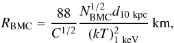 (1)where
(kT)1 keV is the temperature of the thermal emitting
component in units of 1 keV and C = 0.25 for an emitting surface with the
geometry of a circular slab. Equation (1) and
the results of the fit to the total spectrum in Table 1 (where the spectral parameters are better constrained) suggest a radius for the
thermal emitting region of 1 to a few km (for a distance of ~5 kpc; Smith et al. 2012). Such an extended “hot-spot” would be expected in the
case of wind-fed systems accreting at low luminosities (see discussion in Bozzo et al. 2010, and references therein). We note that
at 5 kpc the peak luminosity recorded by XMM-Newton from XTE J1743-363 is
~1035 erg/s. As the temperature of the emitted thermal radiation is about 1–2
keV and the energy coverage of the XMM-Newton data is limited to 12 keV, we
could not well constraint the spectral index α.
(1)where
(kT)1 keV is the temperature of the thermal emitting
component in units of 1 keV and C = 0.25 for an emitting surface with the
geometry of a circular slab. Equation (1) and
the results of the fit to the total spectrum in Table 1 (where the spectral parameters are better constrained) suggest a radius for the
thermal emitting region of 1 to a few km (for a distance of ~5 kpc; Smith et al. 2012). Such an extended “hot-spot” would be expected in the
case of wind-fed systems accreting at low luminosities (see discussion in Bozzo et al. 2010, and references therein). We note that
at 5 kpc the peak luminosity recorded by XMM-Newton from XTE J1743-363 is
~1035 erg/s. As the temperature of the emitted thermal radiation is about 1–2
keV and the energy coverage of the XMM-Newton data is limited to 12 keV, we
could not well constraint the spectral index α.
Even though the BMC model was statistically preferable, a relatively good description of
the data could also be obtained by using a model comprising a power-law and a mekal
component. The latter component accounts in this model for the excess that emerges at
energies ≲2 keV when a simple absorbed power-law model is used to fit the data (see Fig.
3). Similar “soft excesses” have been found in a
number of SFXT sources (Bozzo et al. 2010; Sidoli 2010), SyXBs (Masetti et al. 2006), and are thought to be a ubiquitous characteristic of all NS
accreting X-ray binaries (Hickox et al. 2004). As
discussed in Bozzo et al. (2010), the mekal
component in wind-fed systems with accreting NSs might represent the contribution to
the total X-ray emission from the wind of the companion star. The normalization of the
mekal component can also be translated into an estimate of the size of the
emitting region (see, e.g., Bozzo et al. 2010, and
reference therein): ![Mathematical equation: \begin{equation} R_{\rm mekal}= \sqrt[3]{\frac{3 N_{\rm mekal}}{10^{-14}}\left(\frac{d}{n_{\rm H}}\right)^2} \simeq 7\times10^{13} d_{\rm 5~kpc}^{2/3} a_{\rm 13}^{2/3}~{\rm cm}, \end{equation}](/articles/aa/full_html/2013/08/aa21248-13/aa21248-13-eq94.png) (2)where
d5kpc is the source distance in units of 5 kpc,
nH ~ NH/a,
a13 is the binary separation in units of 1013 cm,
and we made use of the results in Table 1 for
Nmekal and NH. This is consistent
with the soft X-ray emission in XTE J1743-363 being produced in the surroundings of an NS
hosted in a wide binary system. As the orbital period of XTE J1743-363 is not known, it is
not presently possible to assess the applicability of this model. We remark that a similar
soft spectral component was detected during a BeppoSAX observation of the
SyXB 4U 1954+31 and interpreted in the same way (Masetti et
al. 2006).
(2)where
d5kpc is the source distance in units of 5 kpc,
nH ~ NH/a,
a13 is the binary separation in units of 1013 cm,
and we made use of the results in Table 1 for
Nmekal and NH. This is consistent
with the soft X-ray emission in XTE J1743-363 being produced in the surroundings of an NS
hosted in a wide binary system. As the orbital period of XTE J1743-363 is not known, it is
not presently possible to assess the applicability of this model. We remark that a similar
soft spectral component was detected during a BeppoSAX observation of the
SyXB 4U 1954+31 and interpreted in the same way (Masetti et
al. 2006).
In Sect. 2 we analyzed in detail the behavior of the
HR recorded during the XMM-Newton observation. We showed in particular that
the HR underwent a clear change shortly before until after the bright flare, which was
detected about 30 ks after the beginning of the observation. Our analysis showed that there
was an increase of the absorption column density before the onset of the event, followed by
a sudden drop at the peak of the flare for about a few hundreds of seconds. This behavior of
the HR is similar to what was observed during a flare from the SFXT IGR J18410-0535, which
was caught by XMM-Newton in 2011 (Bozzo et
al. 2011). On that occasion the flare was ascribed to an episode of enhanced
accretion onto the NS due to the encounter with a “clump” of material from the stellar wind.
The drop in the absorption column density at the peak of the flare was interpreted as being
due to the photo-ionization of the clump by X-rays from the NS. If a similar interpretation
is applied to the flare from XTE J1743-363, the calculations in Bozzo et al. (2011) suggest in this case a clump radius of
Rcl ~ 2.2 × 10¹⁰vw7 cm,
where we scaled the wind velocity to a value that is more appropriate for an M giant star
(~50–500 km s-1; see, e.g., Espey &
Crowley 2008; Lü et al. 2012, and references
therein). At this low velocity, the accretion radius of the NS is
Racc = 2GM/
 cm and thus becomes larger than the estimated size of the clump6. At variance with the case of IGR J18410-0535, we thus cannot make use here of
the equation
Mcl = Macc(Rcl/Racc)2
from Bozzo et al. (2011). Instead, we have to infer
the mass of the clump directly from the observation, i.e.,
Mcl ≃ Macc. The latter can be
estimated as
Macc = 9 × 10¹⁷
cm and thus becomes larger than the estimated size of the clump6. At variance with the case of IGR J18410-0535, we thus cannot make use here of
the equation
Mcl = Macc(Rcl/Racc)2
from Bozzo et al. (2011). Instead, we have to infer
the mass of the clump directly from the observation, i.e.,
Mcl ≃ Macc. The latter can be
estimated as
Macc = 9 × 10¹⁷ g by using
the observed flare duration of 4.4 ks and integrating over time the unabsorbed flux measured
during the intervals b, c, d, and e in Fig. 5. The
absorption column density caused by the passage of this clump along the line of sight to the
X-ray source is
g by using
the observed flare duration of 4.4 ks and integrating over time the unabsorbed flux measured
during the intervals b, c, d, and e in Fig. 5. The
absorption column density caused by the passage of this clump along the line of sight to the
X-ray source is  mp) ~ 1021
 cm-2, thus suggesting for XTE J1743-363 a particularly low velocity (the
absorption column density measured from the XMM-Newton spectra is
NH ~ 1023 cm-2, see Table 1). We note that complex accretion environments and
inhomogeneous winds in SyXBs were already suggested in the case of 4U 1954+31, where an
X-ray spectrum revealed the presence of multiple and variable absorbers close to the NS
(Mattana et al. 2006; Masetti et al. 2006). As also mentioned for IGR J18410-0535 and other
wind-accreting binaries, the NS magnetic field and rotation might also play a role
regulating the amount of material that can be accumulated and accreted close to the star
magnetospheric boundary (Grebenev & Sunyaev
2007; Bozzo et al. 2008; Postnov et al. 2010). The “magnetic and centrifugal
gates” depend on the local condition at the NS magnetospheric boundary, in particular, on
the magnetic field strength and rotation velocity of the compact object. The lack of
information on the properties of the NS hosted in XTE J1743-363 and the system geometry
(e.g., orbital period, eccentricity) prevent a detailed investigation on how these gates can
affect the parameters of the clump reported above. Further observations of SyXBs with X-ray
instruments endowed with a large collecting area in the soft X-ray domain can help
investigate their flaring behavior in more detail and understand the properties of winds
from cool stars. The candidate ESA mission LOFT (Feroci et
al. 2012) can provide significantly better capabilities in these respects compared
to the present generation of X-ray telescopes. The unprecedented large effective area of its
onboard Large Area Detector (LAD), which operates in the energy range 2–30 keV, will be able
to detect spectral variations during enhanced X-ray emission episodes in bright accreting
binaries down to time scales of few seconds (see also discussion in Bozzo et al. 2013).
cm-2, thus suggesting for XTE J1743-363 a particularly low velocity (the
absorption column density measured from the XMM-Newton spectra is
NH ~ 1023 cm-2, see Table 1). We note that complex accretion environments and
inhomogeneous winds in SyXBs were already suggested in the case of 4U 1954+31, where an
X-ray spectrum revealed the presence of multiple and variable absorbers close to the NS
(Mattana et al. 2006; Masetti et al. 2006). As also mentioned for IGR J18410-0535 and other
wind-accreting binaries, the NS magnetic field and rotation might also play a role
regulating the amount of material that can be accumulated and accreted close to the star
magnetospheric boundary (Grebenev & Sunyaev
2007; Bozzo et al. 2008; Postnov et al. 2010). The “magnetic and centrifugal
gates” depend on the local condition at the NS magnetospheric boundary, in particular, on
the magnetic field strength and rotation velocity of the compact object. The lack of
information on the properties of the NS hosted in XTE J1743-363 and the system geometry
(e.g., orbital period, eccentricity) prevent a detailed investigation on how these gates can
affect the parameters of the clump reported above. Further observations of SyXBs with X-ray
instruments endowed with a large collecting area in the soft X-ray domain can help
investigate their flaring behavior in more detail and understand the properties of winds
from cool stars. The candidate ESA mission LOFT (Feroci et
al. 2012) can provide significantly better capabilities in these respects compared
to the present generation of X-ray telescopes. The unprecedented large effective area of its
onboard Large Area Detector (LAD), which operates in the energy range 2–30 keV, will be able
to detect spectral variations during enhanced X-ray emission episodes in bright accreting
binaries down to time scales of few seconds (see also discussion in Bozzo et al. 2013).
Our long-term monitoring campaign with XRT (see Sect. 3) evidenced a ~40-day period of particularly puzzling low X-ray intensity of the source centered around 56 100 MJD (see Fig. 8). This period was interrupted only by a single flare occurring at ~56 100 MJD (in the corresponding XRT pointing, the source displayed a count-rate of ~2 × 10⁻² cts/s compared to an average count-rate of ~5 × 10⁻³ cts/s in the nearby observations). We note that similar low-intensity episodes were also reported previously by Smith et al. (2012), e.g., around 54 115 MJD. In some of the RXTE observations, the emission recorded by the PCA from the direction of the source was compatible with being due only to Galactic diffuse emission, suggesting that in these periods XTE J1743-363 was in a quiescent state (≪10-11 erg/cm2/s). The latest available PCA observations performed toward the end of the RXTE campaign (from ~55 200 MJD to ~55 300 MJD) also caught XTE J1743-363 again in a low quiescent state (see Fig. 7 in Smith et al. 2012). The Swift pointing ID. 00037884001 that was carried out in the direction of the source at a similar epoch (55 237.82 MJD, see Sect. 3) did not detect any significant X-ray emission and placed a tight upper limit on its flux at 8 × 10-13 erg/cm2/s (2–10 keV). This is compatible with the flux measured by Swift during the low-intensity episode that occurred around 56100 MJD. Outside these two quiescent periods, the fluxes measured by XMM-Newton and Swift are a factor of 5–10 lower than that measured during the latest RXTE observations, which still caught XTE J1743-363 undergoing some residual X-ray activity (~3 × 10-11 erg/cm2/s) around 54 304 MJD. We thus conclude that, besides the overall decreasing trend in the source X-ray emission over the past 15 yrs (Smith et al. 2012), XTE J1743-363 also displays quiescent periods lasting several to tens of days.
Online material
Summary of all Swift /XRT pointings used in this paper.
The EPIC-MOS2 spectrum (operated in timing mode) showed evident instrumental residuals below 2.0 keV and above 8.0 keV, not present in the other spectra of the source. These data were thus discarded for further analysis.
We used the online tool http://www.swift.ac.uk/user_objects/; see Evans et al. (2009).
We neglected in the calculation of Racc the contribution of the NS orbital velocity (see, e.g., Bozzo et al. 2008). For the range of system parameters (masses, orbital periods, and wind velocities) considered here for an SyXB, the NS orbital velocity would be comparable or lower than vw, thus this approximation does not significantly affect our conclusions.
Acknowledgments
We thank the anonymous referee for his/her constructive suggestions, which helped us improve the paper. P.R. acknowledges financial contribution from the contract ASI-INAF I/004/11/0. E.B. acknowledges support from ISSI through funding for the International Team on “Unified View of Stellar Winds in Massive X-ray Binaries” (leader: S. Martínez-Nuñez).
References
- Bird, A. J., Bazzano, A., Bassani, L., et al. 2010, ApJS, 186, 1 [NASA ADS] [CrossRef] [Google Scholar]
- Bozzo, E., Stella, L., Israel, G., Falanga, M., & Campana, S. 2008, MNRAS, 391, L108 [NASA ADS] [CrossRef] [Google Scholar]
- Bozzo, E., Stella, L., Ferrigno, C., et al. 2010, A&A, 519, A6 [NASA ADS] [CrossRef] [EDP Sciences] [Google Scholar]
- Bozzo, E., Giunta, A., Cusumano, G., et al. 2011, A&A, 531, A130 [NASA ADS] [CrossRef] [EDP Sciences] [Google Scholar]
- Bozzo, E., Romano, P., Ferrigno, C., Esposito, P., & Mangano, V. 2013, Adv. Space Res., 51, 1593 [NASA ADS] [CrossRef] [Google Scholar]
- Burrows, D. N., Hill, J. E., Nousek, J. A., et al. 2005, Space Sci. Rev., 120, 165 [NASA ADS] [CrossRef] [Google Scholar]
- Espey, B. R., & Crowley, C. 2008, in RS Ophiuchi (2006) and the Recurrent Nova Phenomenon, eds. A. Evans, M. F. Bode, T. J. O’Brien, & M. J. Darnley, ASP Conf. Ser., 401, 166 [Google Scholar]
- Evans, P. A., Beardmore, A. P., Page, K. L., et al. 2009, MNRAS, 397, 1177 [NASA ADS] [CrossRef] [Google Scholar]
- Feroci, M., Stella, L., van der Klis, M., et al. 2012, Exp. Astron., 34, 415 [NASA ADS] [CrossRef] [Google Scholar]
- Grebenev, S. A., & Sunyaev, R. A. 2007, Astron. Lett., 33, 149 [NASA ADS] [CrossRef] [Google Scholar]
- Hickox, R. C., Narayan, R., & Kallman, T. R. 2004, ApJ, 614, 881 [NASA ADS] [CrossRef] [Google Scholar]
- Israel, G. L., & Stella, L. 1996, ApJ, 468, 369 [NASA ADS] [CrossRef] [Google Scholar]
- Lü, G.-L., Zhu, C.-H., Postnov, K. A., et al. 2012, MNRAS, 424, 2265 [NASA ADS] [CrossRef] [Google Scholar]
- Markwardt, C. B., Swank, J. H., & Marshall, F. E. 1999, IAU Circ., 7120, 1 [NASA ADS] [Google Scholar]
- Masetti, N., Orlandini, M., Palazzi, E., Amati, L., & Frontera, F. 2006, A&A, 453, 295 [NASA ADS] [CrossRef] [EDP Sciences] [Google Scholar]
- Mattana, F., Götz, D., Falanga, M., et al. 2006, A&A, 460, L1 [NASA ADS] [CrossRef] [EDP Sciences] [Google Scholar]
- Postnov, K., Shakura, N., González-Galán, A., et al. 2010, in Eighth Integral Workshop. The Restless Gamma-ray Universe (INTEGRAL 2010) [Google Scholar]
- Ratti, E. M., Bassa, C. G., Torres, M. A. P., et al. 2010, MNRAS, 408, 1866 [NASA ADS] [CrossRef] [Google Scholar]
- Sguera, V., Bazzano, A., Bird, A. J., et al. 2006, ApJ, 646, 452 [NASA ADS] [CrossRef] [Google Scholar]
- Sidoli, L. 2010, AIP Conf. Proc., 1314, 271 [NASA ADS] [CrossRef] [Google Scholar]
- Smith, D. M., Markwardt, C. B., Swank, J. H., & Negueruela, I. 2012, MNRAS, 422, 2661 [NASA ADS] [CrossRef] [Google Scholar]
- Titarchuk, L., Mastichiadis, A., & Kylafis, N. D. 1997, ApJ, 487, 834 [NASA ADS] [CrossRef] [Google Scholar]
All Tables
All Figures
|
Fig. 1 Refined XMM position (1.5′′ at 68% c.l.) of the source reported in the present work is compatible with the Chandra position of the faint source detected by Ratti et al. (0.6′′ at 90% c.l.; 2010) and is suggested to be the quiescent counterpart to XTE J1743-363. We also show the INTEGRAL position (0.7′ at 90% c.l.; Bird et al. 2010) and the Swift /XRT position (2.3′′ at 90% c.l.; see Sect. 3). |
| In the text | |
|
Fig. 2 EPIC-pn lightcurve of XTE J1743-363 in the 0.3–3.5 keV (upper panel) and 3.5–12 keV (lower panel) energy band. The start time is 55 986.8017 MJD and the bin time is 200 s. |
| In the text | |
|
Fig. 3 EPIC-pn (black), EPIC-MOS1 (red), and EPIC-MOS2 (green) spectra of XTE J1743-363 extracted by using the entire exposure time available from the XMM-Newton observation. The best fit is obtained here with an absorbed BMC model. The residuals from this fit are shown in the bottom panel. The middle panel shows the residuals from a fit with a simple power-law model. |
| In the text | |
|
Fig. 4 HID of the source realized by using the same lightcurves shown in Fig. 2 adaptively rebinned to a S/N = 9 (see also Fig. 5). |
| In the text | |
|
Fig. 5 First two panels from the top show the source lightcurves of Fig. 2 rebinned adaptively to a S/N = 9 (based on the lightcurve in the 0.3−3.5 keV energy band). The third panel from the top shows the HR, calculated as the ratio between the source count-rate in the 3.5–12 keV vs. count-rate in the 0.3–3.5 keV energy band. The other three panels show the absorption column density (NH), the power-law photon index (Γ), and the observed flux (units of 10-11 erg/cm2/s) in different time intervals as revealed from our time-resolved spectral analysis (see text for details). |
| In the text | |
|
Fig. 6 Contours plot (68%, 90%, and 99% c.l.) obtained from the fit to the spectra “b” and “d” with the ph*pl and ph*BMC models (see Fig. 5 and Table 1). |
| In the text | |
|
Fig. 7 In the upper part of the plot we show the power spectrum produced using the MOS2 event list as an example. In the bottom part of the plot we show the curves representing the upper limits to the non-detection of pulsations calculated according to Israel & Stella (1996). The solid, dashed and dotted lines correspond to the different sampling times and event list combinations discussed in the text. The two horizontal dashed lines represent the 20% and 30% upper limit levels on the pulsed fraction upper limits as a function of the frequency. The most stringent upper limits we could provide are at 20–30% for frequencies in the range 0.005–200 Hz. |
| In the text | |
|
Fig. 8 Long-term monitoring of XTE J1743-363 performed with Swift /XRT (the campaign started about 50 days after the XMM-Newton observation). The count-rate is given in the 0.3–10 keV energy range. Assuming the source averaged spectral properties reported in Sect. 3, a count-rate of 0.01 cts/s corresponds to about 1.2 × 10⁻¹² erg/cm2/s. Downward arrows correspond to 3σ upperlimits on the source count-rate. |
| In the text | |
|
Fig. 9 Swift /XRT spectrum extracted by summing up all data in Table 2. The best fit is obtained with a simple absorbed power-law model (see text for details). The residuals from this fit are shown in the bottom panel. |
| In the text | |
Current usage metrics show cumulative count of Article Views (full-text article views including HTML views, PDF and ePub downloads, according to the available data) and Abstracts Views on Vision4Press platform.
Data correspond to usage on the plateform after 2015. The current usage metrics is available 48-96 hours after online publication and is updated daily on week days.
Initial download of the metrics may take a while.