| Issue |
A&A
Volume 556, August 2013
|
|
|---|---|---|
| Article Number | A110 | |
| Number of page(s) | 16 | |
| Section | Planets and planetary systems | |
| DOI | https://doi.org/10.1051/0004-6361/201220237 | |
| Published online | 05 August 2013 | |
The HARPS search for southern extra-solar planets⋆,⋆⋆,⋆⋆⋆
XXXIV. A planetary system around the nearby M dwarf GJ 163, with a super-Earth possibly in the habitable zone
1 UJF-Grenoble 1/CNRS-INSU, Institut de Planétologie et d’Astrophysique de Grenoble (IPAG) UMR 5274, 38041 Grenoble, France
e-mail: This email address is being protected from spambots. You need JavaScript enabled to view it.
2 European Southern Observatory, Karl-Schwarzschild-Str. 2, 85748 Garching bei München, Germany
3 Department of Physics, I3N, University of Aveiro, Campus Universitário de Santiago, 3810-193 Aveiro, Portugal
4 Centro de Astrofísica, Universidade do Porto, Rua das Estrelas, 4150-762 Porto, Portugal
5 Observatoire de Genève, Université de Genève, 51 Ch. des Maillettes, 1290 Sauverny, Switzerland
6 Physikalisches Institut, Universitat Bern, Silderstrasse 5, 3012 Bern, Switzerland
7 Institut d’Astrophysique de Paris, CNRS, Université Pierre et Marie Curie, 98bis Bd. Arago, 75014 Paris, France
8 Laboratoire d’Astrophysique de Marseille, UMR 6110 CNRS, Université de Provence, 38 rue Frédéric Joliot-Curie, 13388 Marseille Cedex 13, France
9 Observatoire de Haute-Provence, 04870 Saint-Michel l’ Observatoire, France
10 Institut dAstrophysique et de Géophysique, Université de Liège, Allée du 6 Août 17, Bat. B5C, 4000 Liège, Belgium
11 Astronomie et Systèmes Dynamiques, IMCCE-CNRS UMR 8028, Observatoire de Paris, UPMC, 77 Av. Denfert-Rochereau, 75014 Paris, France
12 Departamento de Física e Astronomia, Faculdade de Ciências, Universidade do Porto, Rua do Campo Alegre, 4169-007 Porto, Portugal
Received: 15 August 2012
Accepted: 4 June 2013
Abstract
The meter-per-second precision achieved by today’s velocimeters enables us to search for 1−10 M⊕ planets in the habitable zone of cool stars. This paper reports on the detection of three planets orbiting GJ 163 (HIP 19394), a M3 dwarf monitored by our ESO/HARPS search for planets. We made use of the HARPS spectrograph to collect 150 radial velocities of GJ 163 over a period of eight years. We searched the radial-velocity time series for coherent signals and found five distinct periodic variabilities. We investigated the stellar activity and called into question the planetary interpretation for two signals. Before more data can be acquired we concluded that at least three planets are orbiting GJ 163. They have orbital periods of Pb = 8.632 ± 0.002, Pc = 25.63 ± 0.03, and Pd = 604 ± 8 days and minimum masses msini = 10.6 ± 0.6, 6.8 ± 0.9, and 29 ± 3 M⊕, respectively. We hold our interpretations for the two additional signals with periods P(e) = 19.4 and P(f) = 108 days. The inner pair presents an orbital period ratio of 2.97, but a dynamical analysis of the system shows that it lays outside the 3:1 mean motion resonance. The planet GJ 163c, in particular, is a super-Earth with an equilibrium temperature of Teq = (302 ± 10)(1 − A)1/4 K and may lie in the so-called habitable zone for albedo values (A = 0.34 − 0.89) moderately higher than that of Earth (A⊕ = 0.2−0.3).
Key words: techniques: radial velocities / stars: late-type / planetary systems / stars: individual: GJ 163
Based on observations made with the HARPS instrument on the ESO 3.6 m telescope under the program IDs 072.C-0488, 082.C-0718, and 183.C-0437 at Cerro La Silla (Chile).
Table 6 is available in electronic form at http://www.aanda.org
Radial-velocity time series (Table 6) are also available at the CDS via anonymous ftp to cdsarc.u-strasbg.fr (130.79.128.5) or via http://cdsarc.u-strasbg.fr/viz-bin/qcat?J/A+A/556/A110
© ESO, 2013
1. Introduction
In the past 15 years or so, we have witnessed impressive progress in radial-velocity measurements. One spectrograph in particular, the High Accuracy Radial velocity Planet Searcher (HARPS; Mayor et al. 2003), broke the former 3 m/s precision barrier and enabled the detection of exoplanets in a yet unknown mass-period domain.
Notably, planets with masses below 10 M⊕ and equilibrium temperatures possibly between ~175–270 K (for plausible albedos) have started to be detected. That subset of detections includes GJ 581d (Udry et al. 2007; Mayor et al. 2009), HD 85512b (Pepe et al. 2011), and GJ 667Cc (Bonfils et al. 2013; Delfosse et al. 2012) which lie in the so-called habitable zone (HZ) of their host star. Depending on the nature of their atmospheres, liquid water may flow on their surface and, because liquid water is thought to be a prerequisite for the emergence of life as we know it, these planets constitute a prized sample for further characterization of their atmosphere and the search for possible biosignatures.
The present paper reports on the detection of at least three planets orbiting the nearby M dwarf GJ 163. One of them, GJ 163c, might be of particular interest in terms of habitability. Our report is structured as follows. Section 2 profiles the host star GJ 163. Section 3 briefly describes the collection of radial-velocity data. Section 4 presents our orbital analysis based on both Markov chain Monte Carlo (MCMC) and periodogram algorithms. Then, we investigate more closely which signal could result from stellar activity rather than from planets (Sect. 5) and retain a solution with three planets. We next investigate the role of planet-planet interactions in the system (Sect. 6) and in particular whether planets b and c participate in a resonance. Section 7 discusses GJ 163c in term of habitability before we present our conclusions in Sect. 8.
2. The properties of GJ 163
The star GJ 163 (HIP 19394, LHS 188) is an M3.5 dwarf (Hawley et al. 1996), at a distance of 15.0 ± 0.4 pc (π = 66.69 ± 1.82 mas; van Leeuwen 2007), and is seen in the Doradus constellation (α = 04h09m16s, δ = −53°22′23′′).
Its photometry (V = 11.811 ± 0.012; K = 7.135 ± 0.021; Koen et al. 2010; Cutri et al. 2003) and parallax imply absolute magnitudes of MV = 10.93 ± 0.14 and MK = 6.26 ± 0.14. The J − K color of GJ 163’s (=0.813; Cutri et al. 2003) and the Leggett et al. (2001) color-bolometric relation result in a K-band bolometric correction of BCK = 2.59 ± 0.07, and in a L⋆ = 0.022 ± 0.002 L⊙ luminosity, in good agreement with the Casagrande et al. (2008) direct determination (Mbol = 8.956; L⋆ = 0.021). The K-band mass-luminosity relation of Delfosse et al. (2000) gives a 0.40 M⊙ mass with a ~10% uncertainty.
Its UVW galactic velocities place GJ 163 between the old disk and halo populations (Leggett 1992). We refined GJ 163’s UVW velocities using both the systemic velocity we measured from HARPS spectra (Table 2) and proper motion from Hipparcos (van Leeuwen 2007). We obtained U = 69.7, V = −76.0, and W = 1.2 km s-1, which confirmed a membership in an old dynamical population.
Stellar metallicity is known to be statistically related to dynamical populations. For the halo population, the metallicity peaks at [Fe/H] ~ − 1.5 (Ryan & Norris 1991) whereas that of the old disk peaks at [Fe/H] ~ − 0.7 (Gilmore et al. 1995). The widths of these distributions are wide, however, and both populations have a small fraction of stars with solar metallicity. Casagrande et al. (2008) attributes a metallicity close to that of the median of the solar neighborhood to GJ 163 ([Fe/H] = − 0.08). And the Schlaufman & Laughlin (2010) photometric relation (or its slight update by Neves et al. 2012) finds a quasi-solar metallicity of [Fe/H] = −0.01. It is therefore difficult to conclude whether GJ 163 belongs to the metal-rich tail of an old population or if it is a younger star accelerated to the typical galactic velocity of an old population.
The star GJ 163 is not detected in the ROSAT All-Sky Survey. We thus used the survey sensitivity limit ( erg/s; Schmitt et al. 1995) to estimate log LX < 5.39 × 1027 erg/s that, given GJ 163’s bolometric luminosity, translates to RX = log LX/LBOL < − 4.17. For an M dwarf of ~0.4 M⊙, the RX versus rotation period of Kiraga & Stepien (2007) gives Prot > 40 days for this level of X flux. To obtain a better estimate of the rotation period we compared Ca H & K chromospheric emission lines of GJ 163 with those of three other M-dwarf planet hosts with comparable spectral types and known rotational periods: GJ 176 (M2V; Prot = 39 d; Forveille et al. 2009), GJ 674 (M2.5V; Prot = 35 d; Bonfils et al. 2007), and GJ 581 (M3V; Prot = 94 d; Vogt et al. 2010). In Fig. 1 we show Ca emission for each star. The star GJ 163 has an activity level close to that of GJ 581 which is a very quiet M dwarf; GJ 163 is much quieter than the 35–40 days rotational period M dwarfs (GJ 176 and GJ 674) and should have a rotational period close to that of GJ 581.
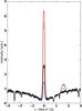 |
Fig. 1 Emission reversal in the Ca ii H line of GJ 674 (red line; M2.5V; Prot = 35 d), GJ 176 (green dots; M2V; Prot = 39 d), GJ 163 (black line; M3.5), and GJ 581 (blue dashes; M3V; Prot = 94 d), ordered from the most prominent to the least prominent peaks. GJ 163 displays a lower activity level, which is a strong indication of slow rotation. |
Observed and inferred stellar parameters for GJ 163.
3. Observations
Modeled and inferred parameters for GJ 163 system.
We observed GJ 163 with HARPS, a fiber-fed spectrograph at the ESO/3.6 m telescope of La Silla Observatory (Mayor et al. 2003; Pepe et al. 2004). Our settings and computation of radial velocities (RV) remained the same as for our guaranteed time observations (GTO) program and we refer the reader to Bonfils et al. (2013) for a detailed description. We gathered RVs for 154 epochs spread over 2988 days (8.2 years) between UT 30 October 2003 and 04 January 2012. Table 6 (available in electronic form) lists all RVs in the barycentric reference frame of the solar system. Four measurements have significantly higher uncertainties: the RVs taken at epochs BJD = 2 454 804.7, 2 455 056.9, 2 455 057.9, and, 2 455 136.8 have uncertainties greater than twice the median uncertainty. We removed them and perform our analysis with the remaining 150 RVs.
The proper motion of GJ 163 (μ = 1.194 ± 0.002 arcsec/yr) implies a secular change in the orientation of its velocity vector. This results in an apparent radial acceleration dv/dt = 0.491 ± 0.013 m s-1 yr-1 (e.g., Kürster et al. 2003), that we subtracted from the RVs listed in Table 6 prior to our analysis. The RV time series is shown in Fig. 2.
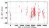 |
Fig. 2 RV time series of GJ 163. |
4. Radial-velocity analysis
The RV variability of GJ163 (σe = 6.31 m/s) is unexplained by photon noise and instrumental errors combined, which are expected to account only for a σi ~ 2.8 m/s dispersion (see Sect. 3 in Bonfils et al. 2013). We therefore analyzed the time series and found that this excess of variability results from up to five different superimposed signals. We describe our analysis below, made in a Bayesian framework using a MCMC algorithm (Sect. 4.1). We also report that similar results are obtained with a classical periodogram analysis (Sect. 4.2).
4.1. MCMC modeling
We used a MCMC algorithm (Gregory 2005, 2007; Ford 2005), which starts with random values for all free parameters of a model, to sample the joint probability distribution of the model parameters. Then this initial solution evolves at the manner of a random walk: each iteration attempts to change the solution randomly, subsequent iterations are accepted following a pseudo-random process, and all accepted solutions form the so-called chain of solutions.
More precisely, for each iteration we generated a new solution and computed its posterior probability. The posterior probability is the product of the likelihood (the probability of observing the data given the parameter values) by the prior probability of the parameter values. The new solution was accepted with a probability that is a function of the ratio between its posterior probability and the posterior probability of the previous solution, such that solutions with a higher posteriori probability were accepted more often. Step-by-step, accepted solutions built a chain that reached a stationary state after enough iterations. We then discarded the first 10 000 iterations and kept only the stationary part of the chain. The distributions of parameter values of all the remaining chain links then corresponded to the targeted joint probability distribution for the model parameters.
Our implementation closely follows that of Gregory (2007); however, we chose to run ten chains in parallel. Each chain was attributed a parameter β that scaled the likelihood such that chains with a lower β value presented a higher acceptance probability. We also paused the MCMC iteration after every ten steps and proposed the chains to permute their solutions (which was again accepted pseudo-randomly and according to the posterior likelihood ratio between solutions). This approach is reminiscent of simulated annealing algorithms and permits evasion outside of local minima and better exploration of the wide parameter space. Only the chain with β = 1 corresponds to the targeted probability distribution. Eventually, we discarded all chains but the one with β = 1. We adopted the median of the posterior distributions for the optimal parameter values, and the 68% centered interval for their uncertainties.
We fitted the data with different models. We chose a model without planets where the sole free parameter was the systemic velocity. We also chose models composed of either one, two, three, four, five, or six planets in Keplerian orbits. We ran our MCMC algorithm to build chains of 500 000 links and eventually removed the first 10 000 iterations.
Table 2 reports optimal parameter values and uncertainties for the model composed of three planets. The parameter values are the median of the posterior distributions and the uncertainties are the 68.3% centered intervals (equivalent to 1-σ for gaussian distributions). Notably, the orbital periods of the three planets are Pb = 8.631 ± 0.002, Pc = 25.63 ± 0.03, and Pd = 604 ± 8 days. Assuming a mass M⋆ = 0.4 M⊙ for the primary, we estimated their minimum masses to msini = 10.6 ± 0.6, 6.8 ± 0.9, and 29 ± 3 M⊕, respectively1. When we fitted the data with a model composed of only one planet we found b, and when we did with a model composed of two planets we found both planets b and d. When we tried a more complex model composed of four or five planets, we recovered the Keplerian orbits described in the three-planet model, as well as Keplerian orbits with periods P(e) = 19.4 and P(f) = 108 days. For the most complex model with six planets, the parameters never converged to a unique solution. The sixth orbit is found with orbital periods around 37, 42, 75, 85, and 134 days and, for a few thousand chain links, the 19.4-day period is not part of the solution but is replaced by one of the orbital periods found for the sixth planet.
More complex models include more free parameters and thus always lead to better fits (i.e., to higher likelihood). To choose whether the improvement in modeling the data justifies the additional complexity, we computed Bayes ratios between the different models. They lead to the posterior probability of one-, two-, and three-planet models over none-, one-, and two-planet models to be as high as 1016, 1011, and 107, respectively, whereas the posterior probabilities for the models with four, five, and six planets over the models with three, four, and five planets were only 75, 62, and 5, respectively. We required that more complex models needed a Bayes ratio >100 to be accepted and thus conclud that our data show strong evidence for at least three planetary signals, and perhaps some evidence for more planets.
4.2. Periodogram analysis
We now present an alternative analysis of the radial-velocity time series based on periodograms. We used floating-mean Lomb-Scargle periodograms (Lomb 1976; Scargle 1982; Cumming et al. 1999) and implemented the algorithm as described in Zechmeister et al. (2009). We chose a normalization such that 1 indicates a perfect fit of the data by a sine wave at a given period whereas 0 indicates no improvement compared to a fit of the data by a constant. To evaluate the false-alarm probability of any peak, we generated faked data sets made of noise only. To make these virtual time series we used bootstrap randomization, i.e., we shuffled the original RVs and retained the date. Shuffling the RVs insures that no coherent signal is present in the virtual time series and keeping the dates conserves the sampling. For each trial we computed a periodogram and measured the power of the highest peak. With 10 000 trials we obtained a distribution of power maxima, which we used as a statistical description for the highest power one can expect if the periodogram was computed on data made of noise only. We searched for the power values that encompassed 68.3%, 95.4%, and 99.7% of the distribution of power maxima (equivalent to 1-, 2-, and 3-σ). A peak found with a power higher than those values (in a periodogram of the original time series) was attributed a false-alarm probability (FAP) lower than 31.7, 4.6, or 0.3%.
We started with a periodogram of the raw RVs. It shows sharp peaks around periods P = 8.6 and 1.13 days (Fig. 3, top panel). They have powers p = 0.50 and 0.41, respectively, much above the power p = 0.21 of a 0.3% FAP. We noted that they were both aliases of each other with our typical one-day sampling and thus tried both periods as starting values for a Keplerian fit. To perform the fit, we used a non-linear minimization with the Levenberg-Marquardt algorithm (Press et al. 1992). We converged on local solutions with reduced χ2 (respectively rms) of 2.52 ± 0.06 (resp. 4.53 m/s) and 3.02 ± 0.06 (resp. 5.02 m/s), respectively. We thus adopted Pb = 8.6 days for the orbital period of the first planet.
We continued by subtracting the Keplerian orbit of planet b to the raw RVs and by doing a periodogram of the residuals (Fig. 3, second panel). We computed a power p = 0.21 for the 0.3% FAP threshold and located eight peaks with more power. They had periods 0.996, 0.999, 1.002, 1.007, 1.038, 25.6, 227 and 625 day, and powers 0.48, 0.30, 0.30, 0.24, 0.30, 0.28, 0.25 and, 0.41, respectively. We identified that several candidates periods are aliases of each other and tried each as a starting value for a Keplerian fit, to a model now composed of two planets. We converged on local solutions with reduced χ2 (resp. rms) of 2.01 (resp. 3.55 m/s), 2.10 (resp. 3.71 m/s), 1.98 (resp. 3.50 m/s), 2.21 (resp. 3.91 m/s), 2.13 (resp. 3.76 m/s), 2.14 (resp. 3.77 m/s), 2.19 (resp. 3.87 m/s), and 1.84 (resp. 3.24 m/s), respectively. Among the peaks with highest significance, the one at P ~ 600 days provided the best fit and we thus adopted this solution.
Next, we pursued the procedure and looked at the residuals around the two-planet solution (Fig. 3, third panel). We recovered some of the previous peaks, with slightly more power excesses (p = 0.30 and 0.28), at periods 25.6 and 1.038 days. We noted again that both periods are probably aliases of each other with the typical one-day sampling. We performed three-planet fit trying both periods as initial guesses for the third planet. We converged on χ2 = 1.50 (rms = 2.59 m/s) and χ2 = 1.53 (rms = 2.66 m/s) for the guessed periods of 25.6 and 1.038 days, respectively. With the periodogram analysis, the solution with Pb = 25.6 days is only marginally favored over the solution with Pb = 1.038 days.
The fourth iteration unveiled one significant power excess around the period 1.006 days (p = 0.22), as well as two other peaks above the two-σ confidence threshold, with periods 19.4 and 108 days (p = 0.16 and 0.14; Fig. 3, fourth panel). We noted that the periods 1.006 and 108 days were aliases under our typical one-day sampling. We tried all three periods (1.006, 19.4, and 108 days) as starting values and converged on χ2 = 1.26 (rms = 2.15 m/s), χ2 = 1.37 (rms = 2.32 m/s), and χ2 = 1.32 (rms = 2.26 m/s), respectively. Again, no period is significantly favored.
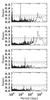 |
Fig. 3 Periodogram analysis of the GJ 163 RV time series, first four iterations. Horizontal lines mark powers corresponding to 31.7, 4.6, and 0.3% false-alarm probability, respectively (i.e., equivalent to 1-, 2-, and 3-σ detections). |
We adopted the solution with Pd = 108 days and computed the periodogram of the residuals. The maximum power is seen again around 19.4 day, now above the three-σ confidence level. Conversely, if we had adopted the solution with Pd = 19.4 days, the period around 108 day (and 1.006 days) would now be the most significant, and above the three-σ threshold too.
Eventually, the sixth iteration unveiled no additional significant power excess. The final five-Keplerian fit has a reduced χ2 = 1.21, for a rms = 2.02 m/s. For reference, we give the orbital elements derived in this section in Table 5 (available in electronic form only).
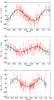 |
Fig. 4 Radial velocity curves for planets b, c, and d, from top to bottom. |
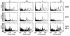 |
Fig. 5 Seasonal periodograms of residual time series obtained after fitting the RV time series with four-planet models. From top to bottom, the rows are for seasons 2008, 2009, and 2010+2011, respectively. From left to right, the columns are periodograms to investigate signals b, (e), c, and (f), respectively. The periodicity of each signal is located with a vertical dashed red line. Power excesses are seen at all seasons for signals b and c, but not for signals (e) and (f). |
5. Challenging the planetary interpretation
At this point, we identified up to five significant signals entangled in the RV data. If not caused by planets orbiting GJ 163, some radial velocity periodic variations could be caused by stellar surface inhomogeneities such as plages or spots. The periodicity is then similar than the orbital period Prot, or might be one of its harmonics Prot/2, Prot/3, etc. (Boisse et al. 2011). Considering the activity of GJ 163 (Sect. 2), we found the rotation is moderate to long, probably greater than two more active stars of our sample, GJ 176 and GJ 674 (i.e., Prot > 35 days), and possibly as long as the rotation period of GJ 581 (~94 d). And therefore, up to three out of the five periodicities identified above might be confused with an activity-induced modulation: the 19.4-, 25.6-, and 108-day periodicities. In this section, we investigated time variability of these signals (Sect. 5.1) and searched for their possible counterparts in various activity indicators (Sect. 5.2).
5.1. Search for changes in RV periodic signals
To explore the possible non-stationarity of one signal, we fitted the data with a model composed of the four other signals and looked at the residuals. In practice, we chose to start the minimization close from the five-planet solution. We used the solution with five planets (Sect. 4.2) and removed from the solution the planet corresponding to the signal we want to study. We then performed a local minimization and computed the residuals, which thus included the signal of interest. Next, we divided the residual time series in three observational seasons (2008, 2009, and 2010+2011). We did not included the observations before 2008 because there are too few and we grouped together 2010 and 2011 data.
We repeated the procedure for all signals except for the longest period (because the ~604-day signal can not be recovered on the time-scale of one season). This produced 4 × 3 = 12 peridograms, shown in Fig. 5. To help locate where the unfitted signal should appear we located its period with a vertical red dashed line.
For both signals b and c, we see clear power excesses at the right periods and for all seasons. This gives further credit that they are the result of orbiting planets. Conversely, the power excess expected for signal (e) is seen in season 2009 only and no power excess is seen for signal (f) in season 2009. This casts doubts on the nature of both signals (e) and (f) and there must be more data before we can draw further conclusions.
5.2. Periodicities in activity indicators
Stellar activity can be diagnosed with spectral indices or by monitoring the shape of the spectral lines, both conveniently measured on the same spectra as those used to measure the radial velocities. We measured 2 spectral indices based on Ca ii H & K lines and on the Hα line, as well as the full width at half maximum (FWHM) and the bisector span (BIS) of the cross-correlation function (CCF). Their values are given in Table 6 along with the radial-velocity measurements.
Among these indicators, we identified a significant periodicity for the FWHM only. Its periodogram indicates some power excess around a period of 30 days, with a false-alarm probability <0.3% (i.e., a confidence level >3σ). We also looked for non stationarity in FWHM and found it is only pseudo-periodic. For instance, in 2008, the maximum power is seen at 30 days, with significant power around 19 days, compatible with the period P(e) identified in RV data. The possible link between this signal with the RV 19.4-day periodicity is however unclear since their strongest power is identified in periodograms of different seasons. We also show the periodogram of FWHM for the 2009 season, where the strongest peak is seen around the period of 38 days (i.e., twice 19 days), albeit with a modest significance.
It is also unclear whether this stellar activity can be linked to the stellar rotation, as a 19- to 38-day rotational period would be short compared to our estimate in Sect. 2.
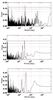 |
Fig. 6 Periodogram of the full width at half maximum of the cross-correlation function for both the whole data set (top panel), season 2008 only (middle panel), and season 2009 (bottom panel). For reference, the period of RV signals are shown with vertical red dashed lines. |
6. Dynamical analysis
After analyzing the RV data with both a MCMC algorithm and with iterative periodograms, we identified up to five superimposed coherent signals. In Sect. 5 we scrutinized several activity indicators and looked for non-stationarity of these signals to finally cast doubts on the planetary nature for two of them. We retained a nominal solution with three planets (Table 2) and now perform a dynamical analysis.
The orbital solution given in Table 2, shows a planetary system composed of three planets, two of them in very tight orbits (ab = 0.06 and ac = 0.13 AU), and another farther away, but in an eccentric orbit, such that the minimum distance at pericenter is only 0.65 AU. The stability of this system is not straightforward, in particular taking into account that the minimum masses of the planets are of the same order as Neptune’s mass. As a consequence, mutual gravitational interactions between planets in the GJ 163 system cannot be neglected and may give rise to some instability.
6.1. Secular coupling
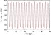 |
Fig. 7 Evolution of the angle Δϖ = ϖb − ϖc (red line) that oscillates around 180° with a maximum amplitude of 28°. The black line also gives the Δϖ evolution, but obtained with the linear secular model (Eq. (2)). |
The ratio between the orbital periods of the two innermost planets determined by the fitting process (Table 2) is Pc/Pb = 2.97, suggesting that the system may be trapped in a 3:1 mean motion resonance. To test the accuracy of this scenario, we performed a frequency analysis of the nominal orbital solution listed in Table 2 computed over 1 Myr. The orbits of the planets are integrated with the symplectic integrator SABA4 of Laskar & Robutel (2001), using a step size of 0.01 yr and including general relativity corrections. We conclude that, in spite of the proximity of the 3:1 mean motion resonance, when we adopt the minimum values for the masses, the two planets in the GJ 163 system are not trapped in this resonance.
The fundamental frequencies of the systems are then the mean motions nb, nc, and nd, and the three secular frequencies of the pericenters g1, g2, and g3 (Table 3). Because of the proximity of the two innermost orbits, there is a strong coupling within the secular system (see Laskar 1990). Both planets b and c precess with the same precession frequency g2, which has a period of 1480 yr. The two pericenters are thus locked and Δϖ = ϖc − ϖb oscillates around 180°, with a maximum amplitude of about 28° (Fig. 7). This behavior is not a dynamical resonance, but merely the result of the linear secular coupling.
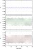 |
Fig. 8 Evolution of the GJ 163 eccentricities with time, starting with the orbital solution from Table 2. The color lines are the complete solutions for the various planets (b: red, c: green, d: blue), while the black curves are the associated values obtained with the linear secular model (Eq. (2)). |
To present the solution more clearerly, it is useful to make a linear change of variables into eccentricity proper modes (see Laskar 1990). In the present case, because of the proximity of the 3:1 mean motion resonance and because of the high value of the outer planet eccentricity, the linear transformation is numerically obtained by a frequency analysis of the solutions. Using the classical complex notation  (1)for
  , we have for the linear Laplace-Lagrange solution
 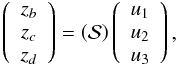 (2)where
  is given by
 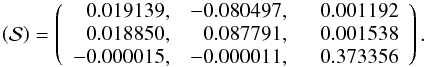 (3)The proper modes uk (with k = 1,2,3) are obtained from the zp by inverting the above linear relation. To a good approximation, we have uk ≈ ei(gkt + φk), where gk and φk are given in Table 3.
From Eq. (2) it is then easy to understand the meaning of the observed libration between the pericenters ϖb and ϖc. Indeed, for both planets b and c, the dominant term is u2 with frequency g2, and they thus both precess with an average value of g2 (black line, Fig. 7).
It should also be noted that Eq. (2) provides good approximations of the long-term evolution of the eccentricities. In Fig. 8 we plot the eccentricity evolution with initial conditions from Table 2. Simultaneously, we plot the evolution of the same elements given by the above secular, linear approximation. The eccentricity variations are very limited and are described well by the secular approximation. The eccentricity of planets b and c are within the ranges 0.061 < eb < 0.101 and 0.067 < ec < 0.109, respectively. These variations are driven mostly by the secular frequency g2, of period approximately 1480 yr (Table 3). The eccentricity of planet d is nearly constant with 0.372 < ed < 0.374 (Fig. 8).
6.2. Stability analysis
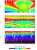 |
Fig. 9 Stability analysis of the nominal fit (Table 2) of the GJ 163 planetary system. For fixed initial conditions, the phase space of the system is explored by varying the semi-major axis ap and eccentricity ep of each planet, b, c, and d, respectively. The step size is 10-5 AU in semi-major axis and 10-2 in eccentricity. For each initial condition, the system is integrated over 200 yr and a stability criterion is derived with the frequency analysis of the mean longitude (Laskar 1990, 1993). As in Correia et al. (2005, 2009, 2010), the chaotic diffusion is measured by the variation in the frequencies. The red zone corresponds to highly unstable orbits, while the dark blue region can be assumed to be stable on a billion-year timescale. The contour curves indicate the value of χ2 obtained for each choice of parameters. |
In order to analyze the stability of the nominal solution (Table 2) and confirm that the inner subsystem is outside of the 3:1 mean motion resonance, we performed a global frequency analysis (Laskar 1993) in the vicinity of this solution, in the same way as achieved for other planetary systems (e.g. Correia et al. 2005, 2009, 2010).
For each planet, the system is integrated on a regular 2D mesh of initial conditions, with varying semi-major axis and eccentricity, while the other parameters are retained at their nominal values (Table 2). The solution is integrated over 200 yr for each initial condition and a stability indicator is computed to be the variation in the measured mean motion over the two consecutive 100 yr intervals of time (for more details see Correia et al. 2005). For regular motion, there is no significant variation in the mean motion along the trajectory, while it can vary significantly for chaotic trajectories. The result is reported in Fig. 9, where “red” represents the strongly chaotic trajectories, and “dark blue” the extremely stable ones.
In Fig. 9 we show the vicinity of the best-fitted solution where the minima of the χ2 level curves correspond to the nominal parameters (Table 2). For the inner system (top and center panels) we observe the presence of the large 3:1 mean motion resonance. We confirm that the present system is outside the 3:1 resonance, in a more stable area at the bottom-right side (Fig. 9, top), or at the bottom-left side (Fig. 9, center). These results are somehow surprising, because if the system had been previously captured inside the 3:1 mean motion resonance, we would expect that the subsequent evolution drive it to the opposite side, where the period ratio is above 3, instead of 2.97. Indeed, during the initial stages of planetary systems, capture in mean motion resonances can occur as a result of orbital migration due to the interactions within a primordial disk of planetesimals, (e.g., Papaloizou 2011). However, as the eccentricities of the planets are damped by tidal interactions with the star, this equilibrium becomes unstable. For first order mean motion resonances it has been demonstrated that the system exits the resonance with a higher period ratio (Lithwick & Wu 2012; Delisle et al. 2012; Batygin & Morbidelli 2013), and this behavior should not differ much for higher order resonances.
For the outer planet (Fig. 9, bottom), we observe that the planet lies in a very stable region. Nevertheless, since the contour curves of minimal χ2 vary smoothly is this zone (unlike those for the inner system), we conclude that this eccentricity may be overestimated. Additional observational data will help to solve this issue, since longer orbital periods become better determined as we acquire data for extended time spans (because we cover more revolutions of the planet around the star). Since the system is already stable with the nominal parameters from Table 2, we do not explore this possibility in great depth in the present paper, but more detailed dynamical studies on this system must take this possibility into account.
We also tested briefly the stability of the five-planet solution (Table 5) and found that it is not stable (even with eccentricities of planets e and f fixed to zero), in particular because of planet e.
6.3. Long-term orbital evolution
From the previous stability analysis, it is clear that the GJ 163 planetary system listed in Table 2 is stable over Gyr timescales. Nevertheless, we also tested directly this by performing a numerical integration of the orbits.
In a first experiment, we integrated the system over 1 Gyr using the symplectic integrator SABA4 of Laskar & Robutel (2001) with a step size of 0.01 yr, including general relativity corrections, but without tidal effects. The result displayed in Fig. 10 show that the orbits evolve in a regular way, and remain stable throughout the simulation, which is of the same order as the age of the star.
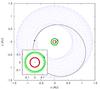 |
Fig. 10 Long-term evolution of the GJ 163 planetary system over 1 Gyr starting with the orbital solution from Table 2. We did not include tidal effects in this simulation. The panel shows a face-on view of the system invariant plane. x and y are spatial coordinates in a frame centered on the star. Present orbital solutions are traced with solid lines and each dot corresponds to the position of the planet every 0.1 Myr. The semi-major axes are almost constant, and the eccentricities present slight variations (0.061 < eb < 0.101, 0.067 < ec < 0.109, and 0.372 < ed < 0.374). |
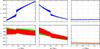 |
Fig. 11 Some possibilities for the long-term evolution of the GJ 163 planetary system over 1 Myr, including tidal effects with Δtp = 105 s. Time scales are inversely proportional to Δt (Eq. (4)), so 1 Myr of evolution roughly corresponds to 1 Gyr with Δtp = 100 s (Qp ~ 103) or 10 Gyr with Δtp = 10 s (Qp ~ 104). We show the ratio Pc/Pb of the orbital periods of the two inner planets (top) and their eccentricities eb (red) and ec (green) (bottom). We use three different sets of initial conditions: Table 2 (left); Table 2 with ac = 0.060679 and Δtc = 5 × 10⁷ s (middle); Table 4 (right). |
Since the two inner planets are very close to the star, in a second experiment we aun a numerical simulation that included tidal effects. Several tidal models have been developed so far, from the simplest ones to the more complex (for a review see Correia et al. 2003; Efroimsky & Williams 2009). The qualitative conclusions are more or less unaffected, so for simplicity we adopt here a linear model with constant Δt (Singer 1968), where Δt is a time delay between the initial perturbation of the planet and the maximal tidal deformation. The tidal force acting on each planet is then given by (Mignard 1979) 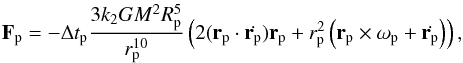 (4)where rp is the position of each planet relative to the star, k2 is the potential Love number, G is the gravitational constant, M is the mass of the star, Rp is the planet radius, and ωp is the spin vector of the planet. Because the spin evolves in a much shorter timescale than the orbit (e.g., Correia 2009), we consider that the spin axis is normal to the orbit, and its norm is given by the equilibrium rotation for a given eccentricity (Eq. (48), Correia et al. 2011)
 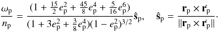 (5)In this experiment we use the ODEX integrator (e.g., Hairer et al. 2011) for the numerical simulations. We adopt k2 = 0.5 and Rp = 0.25 RJup for all planets, and M = 0.4 M⊙ (Table 1). Typical dissipation times for gaseous planets are Δtp ~ 10 to 100 s, corresponding to dissipation factors Qp ~ 104 to 103, respectively (
 ). However, computations with such low Δtp values (or high Qp), become prohibitive on account of long evolution times. In order to speed up the simulations, in this paper we have considered artificially high values for the tidal dissipation, about one thousand times the expected values (Δtp = 105 s or Qp ~ 1). Time scales are inversely proportional to Δtp (Eq. (4)), so 1 Myr of evolution roughly corresponds to 1 Gyr with Δtp = 100 s (or 10 Gyr with Δtp = 10 s).
In Fig. 11 (left) we plot the evolution of the orbital period ratio of the two inner planets together with their orbital eccentricities. We observe that, although the system remains stable, the eccentricities are progressively damped, while the present period ratio increases towards the 3:1 mean motion resonance because of the inward migration of the semi-major axes. Around 0.35 Myr the system crosses the 3:1 resonance, but capture cannot occur because we have a divergent migration (e.g., Henrard & Lamaitre 1983). With a more realistic tidal dissipation (Δtp = 102 s), this event is scheduled to occur in less than 1 Gyr, so we may wonder why the present system is still evolving in such a dramatic way.
One possibility is that the system is already fully evolved by tidal effect, and the eccentricities of the two inner planets are overestimated (see next section). Another possibility is to suppose that planet c is terrestrial, since its minimum mass is 6.8 M⊕ (Table 2). Terrestrial planets usually dissipate much more energy than gaseous planets, with typical values Qp ~ 101 − 102 (e.g. Goldreich & Soter 1966). Thus, adopting Δtc = 5 × 10⁷ s (that is, dissipation for planet c becomes 500 times larger than for the gaseous planets) we repeated the previous simulation, keeping all the other parameters equal, except the initial semi-major axis of this planet ac = 060679 AU. In Fig. 11 (middle) we observe that in this case the orbital period ratio of the two inner planets decreases. Therefore, the system may have crossed the 3:1 resonance in the past, but evolved to the present situation. We adopted ac above the value in the nominal solution (Table 2), so we can see the resonance crossing from above. If we use the nominal value, the orbital period ratio behavior is the same, but decreases to values below the initial 2.97 ratio.
Both the size of the planet and the dissipation rates (Δt) are poorly constrained. More generally, the evolution would be longer for a smaller planet and lower dissipation rates (Eq. (4)). For an Earth composition, planet c minimum mass converts to a radius of roughly 1.7 Rearth (Valencia et al. 2007) and, for the same Δtc, the evolution would take 10 Gyr instead of 1 Gyr. Even for smaller planetary sizes, that scenario would remain possible if Δtc assumed higher values.
6.4. Dissipation constraints
Orbital parameters for the planets orbiting GJ 163, obtained with a tidal constraint for the proper modes u1 and u2.
Fitted orbital solution for the GJ 163 planetary system: 5 Keplerians.
In the previous section we saw that the present orbits of the two inner planets in the GJ 163 are still evolving by tidal effect. Unless the system started with a much higher value for the eccentricities, and depending on its age, the present eccentricities should have already been damped to lower values. In addition, dissipation within a primordial disk should have also contributed to circularize the initial orbits (e.g., Papaloizou 2011). Thus, it is likely that the eccentricities given by the best-fit solution (Table 2) are overestimated, as it is usual when we use insufficient or inaccurate data (e.g., Pont et al. 2011).
One can perform a fit fixing both eccentricities eb and ec at zero. This procedure has been done in many previous works, but as explained in Lovis et al. (2011), it is not a good approach. Indeed, if we do so in the case of the GJ 163 system the subsequent evolution of the eccentricities shows a decoupled system (Δϖ is in circulation), where the eccentricities are mainly driven by angular momentum exchanges with the outer planet, and show some irregular variations.
Over long times, the variations of the planetary eccentricities are usually well described by the secular equations (Eq. (2), Figs. 7 and 8). The best procedure to perform a fit to the observational data that takes into account the eccentricity damping constraint is then to make use of these equations. As for the Laplace-Lagrange linear system (Eq. (2)), we can linearize and average the tidal contribution from expression (4) to the eccentricity, and we obtain for each planet p an additional contribution (Correia et al. 2011) 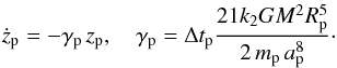 (6)Instead of directly damping the eccentricity, from the previous expression it can be shown that tidal effects damp the proper modes uk as (Laskar et al. 2012)
 ![Mathematical equation: \begin{equation} u_\l \approx \mathrm{e}^{- \tilde \gamma_\l t} \mathrm{e}^{\mathrm{i} \,(g_\l t + \phi_\l)} , \quad \tilde \gamma_\l = [\SS^{-1} \mathrm{diag(\gamma_b,\gamma_c,\gamma_d)} \SS]_{\l \l} . \end{equation}](/articles/aa/full_html/2013/08/aa20237-12/aa20237-12-eq292.png) (7)For the present GJ 163 system, only γb is relevant. However, since the inner system is strongly coupled, both proper modes u1 and u2 are damped with
(7)For the present GJ 163 system, only γb is relevant. However, since the inner system is strongly coupled, both proper modes u1 and u2 are damped with  yr-1 (with Δtb = 100 s), which is compatible with the age of the system. Dissipation in a primordial disk can add some extra contribution to γb, so we expect proper modes u1 and u2 to be considerably damped today. The initial conditions for the GJ 163 planetary system should then take into account this extra information, as has been done for the HD 10180 system (Lovis et al. 2011). We have thus chosen to modify our fitting procedure in order to include a constraint for the tidal damping of the proper modes u1 and u2 using the additional constraint
  (8)For that purpose, we added an additional term to the χ2 minimization corresponding to these proper modes
  (9)where R is a positive constant that is chosen arbitrarily to obtain a small value for u1 and u2 simultaneously. Using R = 50 we get u1 ~ 0.03 and u2 ~ 0.12 and obtain a final
  , which is nearly identical to the results obtained without this additional constraint (R = 0,
  ).
).
The best-fit solution obtained by this method is listed in Table 4. We believe that this solution is a more realistic representation of the true system than the nominal solution (Table 2). Indeed, with this constraint, eccentricity variations of the two innermost planets are regular and slowly damped, while the variations in the ratio of the orbital periods is almost imperceptible (Fig.11, right). In addition, the inner system is still coupled, the two pericentre being locked (Δϖ = ϖc − ϖb oscillates around 180°, with a maximal amplitude of about 26°).
6.5. Additional constraints
We can assume that the dynamics of the three known planets is not disturbed much by the presence of an additional small-mass planet close by. We can thus test the possibility of an additional fourth planet in the system by varying the semi-major axis, the eccentricity, and the longitude of the pericenter over a wide range, and performing a stability analysis as in Fig. 9. The test was completed for a fixed value K = 0.2 m/s, corresponding to an Earth-mass object at approximately 1 AU, whose radial-velocity amplitude is at the edge of detection (Fig. 12).
From the analysis of the stable areas in Fig. 12, one can see that additional planets are possible beyond 2.5 AU (well outside the outer planet’s apocenter), which corresponds to orbital periods longer than 6 yr. Because the eccentricity of the outer planet is high, there are some high-order mean motion resonances that destabilize several zones up to 4 AU. In addition, the same kind of resonances disturb the inner region between planet c and the pericenter of planet d (Fig. 10), although some stability appears to be possible in the range 0.3 < a < 0.5 AU. Stability can also be achieved for planets extremely close to the star, with orbital periods shorter than 8 days.
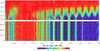 |
Fig. 12 Possible location of an additional fourth planet in the GJ 163 system. The stability of an Earth-size planet (K = 0.2 m/s) is analyzed, for various semi-major axis versus eccentricity (top), or mean anomaly (bottom). All the angles of the putative planet are set to 0° (except the mean anomaly in the bottom panel), and in the bottom panel, its eccentricity to 0. The stable zones where additional planets can be found are the dark blue regions. |
We can also try to find constraints on the maximal masses of the current three-planet system if we assume co-planarity of the orbits. Indeed, up to now we have been assuming that the inclination of the system to the line-of-sight is 90°, which gives minimum values for the planetary masses (Table 2).
By decreasing the inclination of the orbital plane of the system, we increased the mass values of all planets and repeated a stability analysis of the orbits, as in Fig. 9. As we decrease the inclination, the stable dark-blue areas become narrower, to a point that the minimum χ2 of the best-fit solution lies outside the stable zones. At that point, we conclude that the system cannot be stable anymore. It is not straightforward to find a transition inclination between the two regimes, but we can infer from our plots that the stability of the whole system is still possible for an inclination of 30°, but becomes impossible for an inclination of 5° or 10°. Therefore, we conclude that the maximum masses of the planets may be most probably computed for an inclination around 20°, corresponding to a scaling factor of about 3 for the possible masses.
Even when adopting an inclination of 20°, the two inner planets lie outside the 3:1 mean motion resonance, more or less at the same place as for 90° (Fig. 9). The reason why the system becomes unstable for lower inclination values is because the mass of the outer planet d grows to a point such that high order mean motion resonances between planets d and b and/or c destroy the whole system. In particular, the 3:1 resonant island also disappears completely for low inclination values.
7. Gl163c in the habitable zone?
With a separation of 0.1254 AU, GJ 163c receives ~1.34 times more energy from its star than Earth does from the Sun. Considering the case where the whole planetary surface re-radiates the absorbed flux (e.g., β factor of Kaltenegger & Sasselov (2011) equal to 1), the equilibrium temperature of GJ 163c is
![Mathematical equation: $$ T_{\rm eq} = (302\pm10)(1-A)^{1/4} ~~~{[\rm K]}. $$](/articles/aa/full_html/2013/08/aa20237-12/aa20237-12-eq317.png) Scaled to our solar system, its illumination is equivalent to that of a planet located midway between Venus and Earth.
Scaled to our solar system, its illumination is equivalent to that of a planet located midway between Venus and Earth.
To be located in the HZ, and thus potentially harbor liquid water, the equilibrium temperature of a planet with an atmosphere as dense as the Earth’s should be between 175K and 270K (see Selsis et al. 2007, for a complete discussion). In the case of GJ 163c this condition is fulfilled for large range of Bond albedos (A = 0.34 − 0.89), but not for an albedo similar to that of the Earth’s. The albedo of the Earth is equal to 0.3 in the optical and is as low as 0.2 in the near-IR, where early M dwarfs radiate most of their energy. With these values GJ 163c would lie outside the HZ. An albedo greater than 0.34 is, however, possible if 40–50% of the atmosphere is covered by clouds (see, for example, Fig. 1 of Kaltenegger & Sasselov 2011). The precise location of GJ 163c with respect to the habitable zone may further depend on additional heating such as tidal (Barnes et al. 2012) or radiogenic (Ehrenreich et al. 2006) heatings, and more detailed studies are thus welcome.
Two other conditions besides host liquid water on its surface are needed for a planet in the HZ to be truly habitable. First, the planet should not have accreted a massive H-He envelope, otherwise the surface pressure would be too strong and could lead to a runaway greenhouse effect. In the 3–10 M⊕ range, planets can have very different structures for a given mass, and it is impossible to know without a radius measurement whether GJ 163c is embedded in a massive H-He envelope or not. Second, the planet should contain water among the components of its atmosphere.
Numerous discussions exist about two characteristics of planets inside the HZ around M dwarfs and their effect on habitability: their location inside the tidal lock radius of their star and the high activity level of M dwarfs. In Delfosse et al. (2012) we summarized the results of recent works in this domain. The main conclusion is that tidal effect and atmospheric erosion from the neighborhood of active stars does not “preclude the habitability of terrestrial planets orbiting around cool stars (Barnes et al. 2011)”. In particular, the thick atmosphere that may enshroud a planet of ~7 Earth-mass seems stable even around very active M dwarfs (Tian 2009).
8. Conclusion
We have presented the analysis of 150 HARPS RVs of the nearby M dwarf GJ 163 and demonstrated that it encodes at least three signals compatible with the gravitational pull of orbiting planets and identified two additional signals that need further observations before counting them as additional planets. Signals b and d have periodicities that seem incompatible with the possible rotational periods of the star. Signals b and c are also recovered when the data set is divided in observational season, lending credence that at least three planets orbit around GJ 163. We derived their orbital periods (~8.6, 25.6, and 604 days) and their minimum masses (~10.6, 6.8, and 29 M⊕), which correspond to a hot, a temperate, and a cold planet in the super-Earth/Neptune mass regime. The super-Earth GJ 163c may retain further attention for its potential habitability. It receives about 30% more energy than Earth in our solar system and could qualify as a habitable-zone planet for a wide range of albedo values (175 ≤ Teq ≤ 270 K, for 0.34 ≤ A ≤ 0.89).
We also performed a detailed dynamical analysis of the system to show that, despite a period ratio Pc/Pb = 2.97, planets b and c do not participate in a 3:1 resonance. The system is found to be stable over a time comparable to the age of the system and, as far as the orbital parameters of the first three planets remain unchanged, it also appears complete down to Earth-mass planets for a wide range of separations (0.1 ≲ a ≲ 2.2 AU).
The system GJ 163 is singular both for its potentially habitable planet GJ 163c and for its particular hierarchical structure and dynamical history. And therefore, before its atmosphere can be characterized and searched for biomarkers with future observatories, it is already a unique system that connects the potential habitability of a planet with the dynamical history of a planetary system.
Online material
Radial velocity time series of GJ 163 given in the solar system barycentric reference frame (the secular acceleration due to GJ 163 proper motion is not removed), together with measurements of the full width at half maximum (FWHM) and bisector span (BIS) of the cross-correlation function, as well as Ca ii H+K and Hα indices.
An additional ~10% uncertainties should be added quadratically to the mass uncertainty when accounting for the ~10% stellar-mass uncertainty.
Acknowledgments
Our first thanks go to the ESO La Silla staff to whom we are grateful for their continuous support. We wish to thank the anonymous referee for thoughtful comments and suggestions. We also acknowledge support by PNP-CNRS, CS of Paris Observatory, PICS05998 France-Portugal program, Fundação para a Ciência e a Tecnologia (FCT) through program Ciência 2007 funded by FCT/MCTES (Portugal) and POPH/FSE (EC), and by the European Research Council/European Community under the FP7 through a Starting Grant (grants PTDC/CTE-AST/098528/2008, PTDC/CTE-AST/098604/2008, PEst-C/CTM/LA0025/2011, and SFRH/BD/60688/2009), grant agreement 239953. MG is FNRS Research Associate.
References
- Barnes, J. R., Jeffers, S. V., & Jones, H. R. A. 2011, MNRAS, 401, 445 [Google Scholar]
- Barnes, J. R., Jenkins, J. S., Jones, H. R. A., et al. 2012, MNRAS, 3165 [Google Scholar]
- Batygin, K., & Morbidelli, A. 2013, AJ, 145, 1 [NASA ADS] [CrossRef] [Google Scholar]
- Boisse, I., Bouchy, F., Hébrard, G., et al. 2011, A&A, 528, A4 [NASA ADS] [CrossRef] [EDP Sciences] [Google Scholar]
- Bonfils, X., Delfosse, X., Forveille, T., Mayor, M., & Udry, S. 2007, Proc. Conf. In the Spirit of Bernard Lyot: The Direct Detection of Planets and Circumstellar Disks in the 21st Century, June 04–08, 21 [Google Scholar]
- Bonfils, X., Delfosse, X., Udry, S., et al. 2013, A&A, 549, A109 [NASA ADS] [CrossRef] [EDP Sciences] [Google Scholar]
- Casagrande, L., Flynn, C., & Bessell, M. 2008, MNRAS, 389, 585 [NASA ADS] [CrossRef] [MathSciNet] [Google Scholar]
- Correia, A. C. M. 2009, ApJ, 704, L1 [NASA ADS] [CrossRef] [Google Scholar]
- Correia, A. C. M., Laskar, J., & Néron de Surgy, O. 2003, Icarus, 163, 1 [NASA ADS] [CrossRef] [Google Scholar]
- Correia, A. C. M., Udry, S., Mayor, M., et al. 2005, A&A, 440, 751 [NASA ADS] [CrossRef] [EDP Sciences] [Google Scholar]
- Correia, A. C. M., Udry, S., Mayor, M., et al. 2009, A&A, 496, 521 [NASA ADS] [CrossRef] [EDP Sciences] [Google Scholar]
- Correia, A. C. M., Couetdic, J., Laskar, J., et al. 2010, A&A, 511, A21 [NASA ADS] [CrossRef] [EDP Sciences] [Google Scholar]
- Correia, A. C. M., Laskar, J., Farago, F., & Boué, G. 2011, Celest. Mech. Dyn. Astron., 111, 105 [Google Scholar]
- Cumming, A., Marcy, G. W., & Butler, R. P. 1999, ApJ, 526, 890 [NASA ADS] [CrossRef] [Google Scholar]
- Cutri, R. M., Skrutskie, M. F., van Dyk, S., et al. 2003, The IRSA 2MASS All-Sky Point Source Catalog [Google Scholar]
- Delfosse, X., Forveille, T., Ségransan, D., et al. 2000, A&A, 364, 217 [NASA ADS] [Google Scholar]
- Delfosse, X., Bonfils, X., Forveille, T., et al. 2013, A&A, 553, A8 [NASA ADS] [CrossRef] [EDP Sciences] [Google Scholar]
- Delisle, J.-B., Laskar, J., Correia, A. C. M., & Boué, G. 2012, A&A, 546, A71 [NASA ADS] [CrossRef] [EDP Sciences] [Google Scholar]
- Efroimsky, M., & Williams, J. G. 2009, Celest. Mech. Dyn. Astron., 104, 257 [Google Scholar]
- Ehrenreich, D., Lecavelier Des Etangs, A., Beaulieu, J.-P., & Grasset, O. 2006, ApJ, 651, 535 [NASA ADS] [CrossRef] [Google Scholar]
- Ford, E. B. 2005, AJ, 129, 1706 [Google Scholar]
- Forveille, T., Bonfils, X., Delfosse, X., et al. 2009, A&A, 493, 645 [NASA ADS] [CrossRef] [EDP Sciences] [Google Scholar]
- Gilmore, G., Wyse, R. F. G., & Jones, J. B. 1995, AJ, 109, 1095 [NASA ADS] [CrossRef] [Google Scholar]
- Goldreich, P., & Soter, S. 1966, Icarus, 5, 375 [NASA ADS] [CrossRef] [Google Scholar]
- Gregory, P. C. 2005, ApJ, 631, 1198 [NASA ADS] [CrossRef] [Google Scholar]
- Gregory, P. C. 2007, MNRAS, 374, 1321 [NASA ADS] [CrossRef] [Google Scholar]
- Hairer, E., Nørsett, S., & Wanner, G. 2011, Solving Ordinary Differential Equations I: Nonstiff Problems, Springer Series in Computational Mathematics (Springer) [Google Scholar]
- Hawley, S. L., Gizis, J. E., & Reid, I. N. 1996, AJ, 112, 2799 [NASA ADS] [CrossRef] [Google Scholar]
- Henrard, J., & Lamaitre, A. 1983, Celest. Mech., 30, 197 [NASA ADS] [CrossRef] [MathSciNet] [Google Scholar]
- Kaltenegger, L., & Sasselov, D. 2011, ApJ, 736, L25 [NASA ADS] [CrossRef] [Google Scholar]
- Kiraga, M., & Stepien, K. 2007, Acta Astron., 57, 149 [NASA ADS] [Google Scholar]
- Koen, C., Kilkenny, D., van Wyk, F., & Marang, F. 2010, MNRAS, 403, 1949 [Google Scholar]
- Kürster, M., Endl, M., Rouesnel, F., et al. 2003, A&A, 403, 1077 [NASA ADS] [CrossRef] [EDP Sciences] [Google Scholar]
- Laskar, J. 1990, Icarus, 88, 266 [NASA ADS] [CrossRef] [Google Scholar]
- Laskar, J. 1993, Phys. D Nonlinear Phenomena, 67, 257 [Google Scholar]
- Laskar, J., & Correia, A. C. M. 2009, A&A, 496, L5 [NASA ADS] [CrossRef] [EDP Sciences] [Google Scholar]
- Laskar, J., & Robutel, P. 2001, Celest. Mech. Dyn. Astron., 80, 39 [NASA ADS] [CrossRef] [Google Scholar]
- Laskar, J., Boué, G., & Correia, A. C. M. 2012, A&A, 538, A105 [NASA ADS] [CrossRef] [EDP Sciences] [Google Scholar]
- Leggett, S. K. 1992, ApJS, 82, 351 [NASA ADS] [CrossRef] [Google Scholar]
- Leggett, S. K., Allard, F., Geballe, T. R., Hauschildt, P. H., & Schweitzer, A. 2001, ApJ, 548, 908 [NASA ADS] [CrossRef] [Google Scholar]
- Lithwick, Y., & Wu, Y. 2012, ApJ, 756, L11 [NASA ADS] [CrossRef] [Google Scholar]
- Lomb, N. R. 1976, Ap&SS, 39, 447 [NASA ADS] [CrossRef] [Google Scholar]
- Lovis, C., Ségransan, D., Mayor, M., et al. 2011, A&A, 528, A112 [NASA ADS] [CrossRef] [EDP Sciences] [Google Scholar]
- Mardling, R. A. 2007, MNRAS, 382, 1768 [NASA ADS] [Google Scholar]
- Mayor, M., Pepe, F., Queloz, D., et al. 2003, The Messenger, 114, 20 [NASA ADS] [Google Scholar]
- Mayor, M., Bonfils, X., Forveille, T., et al. 2009, A&A, 507, 487 [NASA ADS] [CrossRef] [EDP Sciences] [Google Scholar]
- Mignard, F. 1979, Moon and Planets, 20, 301 [Google Scholar]
- Neves, V., Bonfils, X., Santos, N. C., et al. 2012, A&A, 538, A25 [NASA ADS] [CrossRef] [EDP Sciences] [Google Scholar]
- Papaloizou, J. C. B. 2011, Celest. Mech. Dyn. Astron., 111, 83 [NASA ADS] [CrossRef] [Google Scholar]
- Papaloizou, J. C. B., & Terquem, C. 2010, MNRAS, 405, 573 [NASA ADS] [Google Scholar]
- Pepe, F., Mayor, M., Queloz, D., et al. 2004, A&A, 423, 385 [NASA ADS] [CrossRef] [EDP Sciences] [Google Scholar]
- Pepe, F., Lovis, C., Ségransan, D., et al. 2011, A&A, 534, A58 [NASA ADS] [CrossRef] [EDP Sciences] [Google Scholar]
- Pont, F., Husnoo, N., Mazeh, T., & Fabrycky, D. 2011, MNRAS, 414, 1278 [NASA ADS] [CrossRef] [Google Scholar]
- Press, W. H., Teukolsky, S. A., Vetterling, W. T., & Flannery, B. P. 1992 (Cambridge: University Press) [Google Scholar]
- Ryan, S. G., & Norris, J. E. 1991, AJ, 101, 1865 [NASA ADS] [CrossRef] [Google Scholar]
- Scargle, J. D. 1982, ApJ, 263, 835 [NASA ADS] [CrossRef] [Google Scholar]
- Schlaufman, K. C., & Laughlin, G. 2010, A&A, 519, A105 [NASA ADS] [CrossRef] [EDP Sciences] [Google Scholar]
- Schmitt, J. H. M. M., Fleming, T. A., & Giampapa, M. S. 1995, AJ, 450, 392 [Google Scholar]
- Selsis, F., Kasting, J. F., Levrard, B., et al. 2007, A&A, 476, 1373 [NASA ADS] [CrossRef] [EDP Sciences] [Google Scholar]
- Singer, S. F. 1968, Geophys. J. R. Astron. Soc., 15, 205 [CrossRef] [Google Scholar]
- Tian, F. 2009, ApJ, 703, 905 [NASA ADS] [CrossRef] [Google Scholar]
- Udry, S., Bonfils, X., Delfosse, X., et al. 2007, A&A, 469, L43 [NASA ADS] [CrossRef] [EDP Sciences] [Google Scholar]
- Valencia, D., Sasselov, D. D., & O’Connell, R. J. 2007, ApJ, 665, 1413 [NASA ADS] [CrossRef] [Google Scholar]
- van Leeuwen, F. 2007, A&A, 474, 653 [NASA ADS] [CrossRef] [EDP Sciences] [Google Scholar]
- Vogt, S. S., Butler, R. P., Rivera, E. J., et al. 2010, ApJ, 723, 954 5733 [NASA ADS] [CrossRef] [EDP Sciences] [Google Scholar]
- Zechmeister, M., Kürster, M., & Endl, M. 2009, A&A, 505, 859 [NASA ADS] [CrossRef] [EDP Sciences] [Google Scholar]
All Tables
Orbital parameters for the planets orbiting GJ 163, obtained with a tidal constraint for the proper modes u1 and u2.
Radial velocity time series of GJ 163 given in the solar system barycentric reference frame (the secular acceleration due to GJ 163 proper motion is not removed), together with measurements of the full width at half maximum (FWHM) and bisector span (BIS) of the cross-correlation function, as well as Ca ii H+K and Hα indices.
All Figures
|
Fig. 1 Emission reversal in the Ca ii H line of GJ 674 (red line; M2.5V; Prot = 35 d), GJ 176 (green dots; M2V; Prot = 39 d), GJ 163 (black line; M3.5), and GJ 581 (blue dashes; M3V; Prot = 94 d), ordered from the most prominent to the least prominent peaks. GJ 163 displays a lower activity level, which is a strong indication of slow rotation. |
| In the text | |
|
Fig. 2 RV time series of GJ 163. |
| In the text | |
|
Fig. 3 Periodogram analysis of the GJ 163 RV time series, first four iterations. Horizontal lines mark powers corresponding to 31.7, 4.6, and 0.3% false-alarm probability, respectively (i.e., equivalent to 1-, 2-, and 3-σ detections). |
| In the text | |
|
Fig. 4 Radial velocity curves for planets b, c, and d, from top to bottom. |
| In the text | |
|
Fig. 5 Seasonal periodograms of residual time series obtained after fitting the RV time series with four-planet models. From top to bottom, the rows are for seasons 2008, 2009, and 2010+2011, respectively. From left to right, the columns are periodograms to investigate signals b, (e), c, and (f), respectively. The periodicity of each signal is located with a vertical dashed red line. Power excesses are seen at all seasons for signals b and c, but not for signals (e) and (f). |
| In the text | |
|
Fig. 6 Periodogram of the full width at half maximum of the cross-correlation function for both the whole data set (top panel), season 2008 only (middle panel), and season 2009 (bottom panel). For reference, the period of RV signals are shown with vertical red dashed lines. |
| In the text | |
|
Fig. 7 Evolution of the angle Δϖ = ϖb − ϖc (red line) that oscillates around 180° with a maximum amplitude of 28°. The black line also gives the Δϖ evolution, but obtained with the linear secular model (Eq. (2)). |
| In the text | |
|
Fig. 8 Evolution of the GJ 163 eccentricities with time, starting with the orbital solution from Table 2. The color lines are the complete solutions for the various planets (b: red, c: green, d: blue), while the black curves are the associated values obtained with the linear secular model (Eq. (2)). |
| In the text | |
|
Fig. 9 Stability analysis of the nominal fit (Table 2) of the GJ 163 planetary system. For fixed initial conditions, the phase space of the system is explored by varying the semi-major axis ap and eccentricity ep of each planet, b, c, and d, respectively. The step size is 10-5 AU in semi-major axis and 10-2 in eccentricity. For each initial condition, the system is integrated over 200 yr and a stability criterion is derived with the frequency analysis of the mean longitude (Laskar 1990, 1993). As in Correia et al. (2005, 2009, 2010), the chaotic diffusion is measured by the variation in the frequencies. The red zone corresponds to highly unstable orbits, while the dark blue region can be assumed to be stable on a billion-year timescale. The contour curves indicate the value of χ2 obtained for each choice of parameters. |
| In the text | |
|
Fig. 10 Long-term evolution of the GJ 163 planetary system over 1 Gyr starting with the orbital solution from Table 2. We did not include tidal effects in this simulation. The panel shows a face-on view of the system invariant plane. x and y are spatial coordinates in a frame centered on the star. Present orbital solutions are traced with solid lines and each dot corresponds to the position of the planet every 0.1 Myr. The semi-major axes are almost constant, and the eccentricities present slight variations (0.061 < eb < 0.101, 0.067 < ec < 0.109, and 0.372 < ed < 0.374). |
| In the text | |
|
Fig. 11 Some possibilities for the long-term evolution of the GJ 163 planetary system over 1 Myr, including tidal effects with Δtp = 105 s. Time scales are inversely proportional to Δt (Eq. (4)), so 1 Myr of evolution roughly corresponds to 1 Gyr with Δtp = 100 s (Qp ~ 103) or 10 Gyr with Δtp = 10 s (Qp ~ 104). We show the ratio Pc/Pb of the orbital periods of the two inner planets (top) and their eccentricities eb (red) and ec (green) (bottom). We use three different sets of initial conditions: Table 2 (left); Table 2 with ac = 0.060679 and Δtc = 5 × 10⁷ s (middle); Table 4 (right). |
| In the text | |
|
Fig. 12 Possible location of an additional fourth planet in the GJ 163 system. The stability of an Earth-size planet (K = 0.2 m/s) is analyzed, for various semi-major axis versus eccentricity (top), or mean anomaly (bottom). All the angles of the putative planet are set to 0° (except the mean anomaly in the bottom panel), and in the bottom panel, its eccentricity to 0. The stable zones where additional planets can be found are the dark blue regions. |
| In the text | |
Current usage metrics show cumulative count of Article Views (full-text article views including HTML views, PDF and ePub downloads, according to the available data) and Abstracts Views on Vision4Press platform.
Data correspond to usage on the plateform after 2015. The current usage metrics is available 48-96 hours after online publication and is updated daily on week days.
Initial download of the metrics may take a while.