| Issue |
A&A
Volume 555, July 2013
|
|
|---|---|---|
| Article Number | A46 | |
| Number of page(s) | 14 | |
| Section | Stellar atmospheres | |
| DOI | https://doi.org/10.1051/0004-6361/201321584 | |
| Published online | 27 June 2013 | |
Discovery of the magnetic field in the pulsating B star β Cephei ⋆,⋆⋆
1
Astronomical Institute “Anton Pannekoek”, University of
Amsterdam, Science Park
904, 1098 XH
Amsterdam, The
Netherlands
e-mail: h.f.henrichs@uva.nl
2
European Space Agency (ESAC), PO Box 78, 28691 Villanueva de la
Cañada, Madrid,
Spain
3
LESIA, Observatoire de Paris, CNRS UMR 8109, UPMC, Université
Paris Diderot, 5 place Jules
Janssen, 92190
Meudon,
France
4
Observatoire Midi-Pyrénées, 14 Avenue Edouard Belin, 31400
Toulouse,
France
5
LESIA, Observatoire de Paris, CNRS, UPMC, Université Paris
Diderot, Place Jules
Janssen, 92190
Meudon,
France
6
Physics and Astronomy Department, The University of Western
Ontario, London,
Ontario, N6A 3K7, Canada
7
Department of Physics, Royal Military College of Canada, PO Box 17000, Kingston, Ontario, K7K
7B4, Canada
8
Max Planck Institute for Extraterrestrial Physics,
Giessenbachstraße, 85748
Garching bei München,
Germany
9
Harvard–Smithsonian Center for Astrophysics,
60 Garden Str., Cambridge, MA
02138,
USA
10
European Space Astronomy Center, Villanueva de la Cañada, 28691
Madrid,
Spain
11
W. M. Keck Observatory, 65-1120 Mamalahoa Highway, Kamuela, HI
96743,
USA
Received: 27 March 2013
Accepted: 22 April 2013
Context. Although the star itself is not helium enriched, the periodicity and the variability in the UV wind lines of the pulsating B1 IV star β Cephei are similar to what is observed in magnetic helium-peculiar B stars, suggesting that β Cep is magnetic.
Aims. We searched for a magnetic field using high-resolution spectropolarimetry. From UV spectroscopy, we analysed the wind variability and investigated the correlation with the magnetic data.
Methods. We used 130 time-resolved circular polarisation spectra that were obtained from 1998 (when β Cep was discovered to be magnetic) to 2005, with the MuSiCoS échelle spectropolarimeter at the 2 m Télescope Bernard Lyot. We applied the least-square deconvolution method on the Stokes V spectra and derived the longitudinal component of the integrated magnetic field over the visible hemisphere of the star. We performed a period analysis on the magnetic data and on equivalent-width measurements of UV wind lines obtained over 17 years. We also analysed the short- and long-term radial velocity variations, which are due to the pulsations and the 90-year binary motion, respectively.
Results. β Cep hosts a sinusoidally varying magnetic field with an amplitude 97 ± 4 G and an average value − 6 ± 3 G. From the UV wind line variability, we derive a period of 12.00075(11) days, which is the rotation period of the star, and is compatible with the observed magnetic modulation. Phases of maximum and minimum field match those of maximum emission in the UV wind lines, strongly supporting an oblique magnetic-rotator model. We discuss the magnetic behaviour as a function of pulsation behaviour and UV line variability.
Conclusions. This paper presents the analysis of the first confirmed detection of a dipolar magnetic field in an upper main-sequence pulsating star. Maximum wind absorption originates in the magnetic equatorial plane. Maximum emission occurs when the magnetic north pole points to the Earth. Radial velocities agree with the ~90-year orbit around its Be-star binary companion.
Key words: magnetic fields / stars: winds, outflows / binaries: spectroscopic / stars: oscillations / stars: early-type
Based on observations obtained using the MuSiCoS spectropolarimeter at the Observatoire du Pic du Midi and by the International Ultraviolet Explorer, which were collected at NASA Goddard Space Flight Center and Villafranca Satellite Tracking Station of the European Space Agency.
Table 2 is available in electronic form at http://www.aanda.org
© ESO, 2013
1. Introduction
The star β Cephei (HR 8238, HD 205021, HIP 106032, WDS 21287+7034) was classified as a spectral type B1 III by Lesh (1968), but earlier references suggest that it may be type B2 III or B1 IV. Morel et al. (2006) assigned it a revised spectral type of B1 Vevar. The Be status of this star was dismissed by Schnerr et al. (2006a), who unambiguously demonstrated by spectroastrometry that the intermittent Hα emission often encountered in spectra of β Cep originates in the companion star (with spectral type B6–8) that is 3.4-mag fainter and mostly only speckle-resolved. This companion was discovered with the 200-inch Hale telescope by Gezari et al. (1972), and its orbit with an approximate period of 90 y was subsequently determined by Pigulski & Boratyn (1992). More properties of this companion have been studied by Wheelwright et al. (2009). The star β Cephei is the prototype of the β Cephei class of pulsating stars (Frost & Adams 1903). Its multi-periodic photometric and spectroscopic line-profile variability have been studied extensively (Heynderickx et al. 1994; Telting et al. 1997; Shibahashi & Aerts 2000). In addition to the main pulsation period of 4h 34m, the star exhibits a very significant period of 12 d in the equivalent width of the ultraviolet resonance lines. At the time of its discovery by Fischel & Sparks (1972) with the OAO-2 satellite, which was confirmed and further investigated by Panek & Savage (1976), the period had not been precisely determined (6 or 12 days). Later investigations with IUE data (Henrichs et al. 1993, 1998) left no doubt that the two minima in equivalent width of the C iv stellar wind lines, which are separated by 6 d, are unequal, and that the real period is 12 d. Henrichs et al. (1993) proposed that the UV periodicity arises from the 12-day rotational period of the star and suggested that the stellar wind is modulated by an oblique dipolar magnetic field at the surface. A rotational period of 12 days corresponds well with an adopted radius between six and ten solar radii, given the reported values of 20–27 km s-1 for vsini (Abt et al. 2002; Telting et al. 1997).
Support for this hypothesis was provided by the striking similarity between the UV-line behaviour of β Cep and of well-known, chemically peculiar magnetic B stars, such as the B2 V helium-strong star HD 184927 (Barker et al. 1982; Wade et al. 1997). See Henrichs et al. (2012) for a comparison. A reported (but not confirmed) average magnetic field strength of B = (810 ± 170) G for β Cep itself was published by Rudy & Kemp (1978), which is based on data between 1975 and 1976. This was however a marginal detection with only one point above the 3σ level. It is unlikely that this result was affected by contaminating emission, because the Hγ line was mostly used, which was never observed in emission. According to the compilation of Pan’ko & Tarasov (1997), the system was not likely in an emission state during these years.
To verify the magnetic hypothesis, Henrichs et al. (1993) presented new magnetic field measurements which were obtained by one of us (GH), with the University of Western Ontario photoelectric Pockels cell polarimeter and 1.2m telescope that were simultaneously measured with UV spectroscopy with the IUE satellite. The technique used to measure the magnetic field was differential circular polarimetry in the Hβ line (Landstreet 1982 and references therein). The 12-day UV period in the equivalent width of the stellar wind lines of C iv, Si iii, Si iv, and N v was confirmed, but the values for the magnetic field with 1σ error bars of about 150 G which are comparable to the measured field strength, were much lower than the value reported by Rudy & Kemp (1978). However, additional magnetic measurements with the same instrumentation by G. Hill and G. Wade (see Fig. 1) could not confirm the 12-day period which was unexplained. It remained puzzling why these new magnetic field measurements indicated a much lower field than in 1978. It was suggested that the new Be phase of the star, which was discovered in July 1990 by Mathias et al. (1991; see also Kaper et al. 1992; Kaper & Mathias 1995), might have been related to the decrease in magnetic field strength. This hypothesis could not be tested and has since been made obsolete because Schnerr et al. (2006a) discovered that the emission stems from the binary companion. One possible explanation of the discordance between the magnetic field measurements from the Hβ line and those given below is that Hβ may have been partially filled in with emission during the time of the observations, because Hα was in emission at that time.
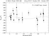 |
Fig. 1 Early magnetic measurements of β Cep, which are obtained with the University of Western Ontario photoelectric Pockels cell polarimeter and 1.2m telescope. Typical exposure times were between 1 and 3.5 h. The dashed curve is the best sinusoid fit, based on the analysis of all data points in this paper, and is the same as in Fig. 6. |
These considerations motivated us to undertake new magnetic measurements of β Cep with the much more sensitive MuSiCoS polarimeter at the Pic du Midi observatory in France. Using this instrument has the clear advantage that all available (mostly metallic) magnetically sensitive lines can be selected in the spectrum, instead of just one Balmer line, which may be contaminated with some emission. This paper presents and discusses the observed measurements and analyses the correlation between the magnetic, pulsational, and UV behaviour.
The magnetic field of β Cep was first measured on December 13, 1998 and was followed by 22 observations in January 1999 and June/July 1999, such that the rotational period was sufficiently covered to allow a thorough assessment. In an earlier stage of writing the current paper, we decided to separately publish the model calculations based on these first 23 measurements (Donati et al. 2001), which would take much less time to complete in view of the extended data analysis and difficult interpretation of the odd behaviour of the variable Hα emission to follow. In that paper, we also included a discussion of the stellar parameters, which we have summarized in Table 1, except for the Hipparcos distance that was revised by van Leeuwen (2007). The model calculations were constrained by the observed X-ray emission, as observed by Berghöfer et al. (1996). Donati et al. (2001) also devoted a discussion to possible implications of the magnetic field of β Cep for understanding the Be phenomenon, which now appears to be academic for this star. As the variability of the Hα line stems from the companion of β Cep, we do not discuss this aspect in the current paper (For a summary, see Wheelwright et al. 2009.).
In Sect. 2, we describe the experimental setup and the observations. Sect. 3 summarizes the data reduction and the results. In Sect. 4, we derive the system velocity and compare the known periodicities in β Cep with the magnetic measurements. In the last section, we give our conclusions and discuss the implications of the current measurements, including a discussion of recent interferometric and X-ray measurements.
2. Experimental setup and observations
We obtained circular polarisation (Stokes V) and total intensity (Stokes I) of β Cep, using the MuSiCoS spectropolarimeter mounted on the 2-m Télescope Bernard Lyot (TBL) at the Observatoire du Pic du Midi. The strategy of the observations was fourfold: (1) to cover the known 12-day period of the UV lines; (2) to have reasonable coverage during one pulsational period of 4.6 h; (3) to study the magnetic and pulsational behaviour on a yearly timescale; and (4) to investigate the systemic radial velocity of the star in its 90-year orbit. The journal of observations is given in Table 2.
The spectropolarimetric setup consisted of the MuSiCoS fiber-fed cross dispersed échelle spectrograph (Baudrand & Bohm 1992; Catala et al. 1993) with a dedicated polarimetric unit (described by Donati et al. 1999) mounted at the Cassegrain focus. The light passes through a rotatable quarter wave plate, converting the circular polarisation into linear, after which the beam is split into two beams with a linear polarisation along and perpendicular to the instrumental reference azimuth. Two fibers transport the light to the spectrograph, where both orthogonal polarisation states are simultaneously recorded. The spectral coverage in one exposure is from 450 to 660 nm with a resolving power of about 35 000. The Site CCD detector with 1024 × 1024 of 24 μ pixels was used, which has a quantum efficiency exceeding 50% in the U band.
A complete Stokes V measurement consists of four subsequent subexposures between which the quarter wave plate is rotated, so that a sequence is obtained with −45/45/45/−45 degrees angle (called the q1-q3-q3-q1 sequence). This results in exchange of the two beams throughout the whole instrument. With this sequence, all systematic spurious circular polarisation signals down to 0.002% rms can be suppressed (Donati et al. 1997, 1999; Wade et al. 2000). At the beginning and at the end of each night, we took 15 flatfield exposures, whereas the usual bias frames and polarisation check exposures, and wavelength calibrations with a Th-Ar lamp were taken several times per night. For the reduction, we used the flatfield series averaged over the night, where we separated the flatfields taken in the q1 and q3 orientation.
3. Data reduction and results
The data reduction was done with the dedicated ESpRIT reduction package, described by Donati et al. (1997). We used a slightly modified version
in which the separated q1 and q3 flatfields are used. With
this package, the geometry of the orders on the CCD is first determined, and after an
automatic wavelength calibration on the Th-Ar frames, a rigorous optimal extraction of the
orders is performed. The method we used to calculate the magnetic field strength includes a
least-squares deconvolution (LSD) to calculate a normalised average Stokes
I line profile and corresponding Stokes V line profiles.
This magnetic field strength calculation uses as many possible spectral lines. The presence
of a magnetic field will result in a typical Zeeman signature in the average Stokes
V profile, from which the effective longitudinal component
(Bℓ) of the stellar magnetic field can be
determined. This is done by taking the first-order moment using the well-known relation
(Mathys 1989; Donati et al. 1997), ![\begin{equation} \label{equ:bl} B_{\ell} = (-2.14\times 10^{11}~{\rm G})\frac{\int vV(v) {\rm d}v} {\lambda g c\int [1 - I(v)] {\rm d}v}, \end{equation}](/articles/aa/full_html/2013/07/aa21584-13/aa21584-13-eq32.png) (1)where λ, in nm, is the mean
wavelength, c is the velocity of light in the same units as the velocity
v, and g is the mean value of the Landé factors of all
lines used to construct the LSD profile. We used λ = 512.5 nm and
g = 1.234. The noise in the LSD spectra was measured and given in Table
2, along with the signal-to-noise ratio (S/N)
obtained in the raw data. The profiles were normalised outside the regions of [−120, 120] km
s-1.
(1)where λ, in nm, is the mean
wavelength, c is the velocity of light in the same units as the velocity
v, and g is the mean value of the Landé factors of all
lines used to construct the LSD profile. We used λ = 512.5 nm and
g = 1.234. The noise in the LSD spectra was measured and given in Table
2, along with the signal-to-noise ratio (S/N)
obtained in the raw data. The profiles were normalised outside the regions of [−120, 120] km
s-1.
Considerations of several important effects appeared decisive for the final outcome of the magnetic results. The absolute values of Bℓ are impacted by: fringe patterns, which are present in many spectra; the selection of spectral lines for the LSD analysis; the limits of integration in Eq. (1); and the asymmetry of the lines thanks to the pulsation, which we discuss in turn.
3.1. Correction for fringes
Many Stokes V spectra appeared to be strongly affected by interference fringes that are to likely originate in the quarter-wave plate. These fringes could induce a spurious Zeeman detection that could modify the value of the measured longitudinal magnetic field. We have eliminated the fringes from the spectra using a Stokes V spectrum of a bright star that carried no detectable Zeeman signature. We used spectra of Vega during the same observing run for all but two datasets. For the 2001 data, we used ζ Oph. We could not apply the fringe correction to the dataset obtained in June 2000, because no suitable spectrum of Vega or a similar star was available. This template spectrum is smoothed with a running mean of 10 or 20 points to remove any possible features that could modify the β Cep Stokes V spectra during the correction process. In this way, we assure that only the (sine-like wave) fringe pattern remains. The spectra to be corrected are then divided by the template. The method is illustrated in Fig. 2 showing an overplot of the smoothed Vega spectrum and the Stokes V spectrum nr. 22 (1999) of β Cep, with the resulting spectrum. After application of this procedure, the error bars improved by typically 10% to 20%, whereas the resulting magnetic values shifted dramatically by more than 50 G in some cases, which showed the necessity to correct for the fringes. Table 3 gives numerical examples, including the cumulative effects of the selected line list, as discussed below. We note that Wade et al. (2006) used a wavelet transform procedure to remove the fringe patterns by using the same spectrum of Vega in 2003 to analyse the spectra of α And.
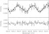 |
Fig. 2 Top: overplot of a smoothed Stokes V spectrum of Vega (dashed line) and a Stokes V spectrum of β Cep (1999, nr. 22). Both contain a strong spurious modulation caused by fringing on the CCD. Bottom: Stokes V spectrum of β Cep after removal of the fringes. |
3.2. Effect of the spectral line list
The profiles of 125 relatively weak lines, which are selected with a table appropriate for early B stars, were combined by means of the LSD method, as described above in the interval [−243, 243] km s-1. Many of these lines are blends of multiplets, leaving effectively 77 distinct lines. The selection of lines included in the construction of the LSD profiles appear to have a systematic influence on the absolute value of the magnetic field. The removal of blends from the list resulted in a larger absolute signal. We also investigated the effect of using measured instead of theoretically calculated line depths. The smallest error bar, which likely resulted in the most reliable value for Bℓ, is obtained when fringe correction is applied, strong blends are excluded, and measured line depths are used, as illustrated in Table 3.
Illustrative sample calculations of magnetic-field strength without and with fringe correction and with different selections of spectral lines and weights (line depths) used for the construction of the LSD Stokes V profile.
3.3. Limits of integration and asymmetry
 |
Fig. 3 Representative LSD Stokes unpolarised I (lower panel) and circularly polarised V (upper panel) profiles of β Cep from top to bottom on 15 and 18 December 1998, 15 January, and 3 July 1999. The signal- to-noise ratio (S/N) per velocity bin in the raw data is indicated. Note the clear Zeeman signatures at the zero, positive, and negative fields. The two lower figures illustrate negative fields at almost opposite pulsation phases. In Sect. 4, we show that the pulsation phase does not affect the magnetic field determination. |
Applying Eq. (1) to calculate Bℓ involves taking the first moment, which implies measuring the asymmetry with respect to the centre of the profile. A shift in the radial velocity scale will therefore affect the value of the magnetic field, and a proper correction is essential. Because the radial velocity amplitude is considerable as a consequence of the pulsation of β Cep, we shifted the minima of the I profiles (at vmin, which are determined by a parabola fit to the points near the minimum intensity) to zero velocity before calculating the longitudinal field strength. The profiles are often asymmetric, implying that the minimum flux does not occur at the radial velocity (vrad) of the star. The velocity was measured using the first moment of the profile with respect to the barycentric restframe, which is normalised by the equivalent width (we followed Schrijvers et al. 1997). The measured values of vmin and vrad are included in Table 2.
We approximated the integral in Eq. (1) by
a simple summation in a range between ± vlimit and computed
the uncertainties as follows: 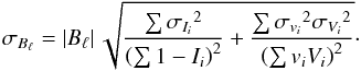 (2)The limits of the integral in Eq. (1) were carefully determined to minimize the
uncertainties. We first computed the Bℓ
values for 17 different limits between 10 and 90 km s-1. The full Zeeman
signature is obtained when the maximum value for
Bℓ is reached. We adopted the average
optimum value of several test cases, which was at vlimit = 54
km s-1.
(2)The limits of the integral in Eq. (1) were carefully determined to minimize the
uncertainties. We first computed the Bℓ
values for 17 different limits between 10 and 90 km s-1. The full Zeeman
signature is obtained when the maximum value for
Bℓ is reached. We adopted the average
optimum value of several test cases, which was at vlimit = 54
km s-1.
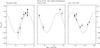 |
Fig. 4 The discovery observations, which include the first 23 datapoints from December 1998 until July 1999. The longitudinal component of the averaged surface magnetic field of β Cep is plotted. The dashed curve is the best-fit sine curve for all magnetic data with a fixed period of 12.00075 d, as derived from UV data. |
We have also investigated the effect of the asymmetry of the lines (because of the pulsation) by varying the reference centre. We find that a displacement of more than ±18 km s-1 gives significant lower values for the field strength, but the determined values and the error bars remain constant within 4% within this range. For typical examples of Zeeman LSD profiles (i.e. the Stokes I and V spectrum in velocity space), see Fig. 3. In this figure, we show the LSD profiles for a zero, positive, and negative field, where the latter are at two different pulsation phases of the star (see below).
We also calculated diagnostic null (or N) spectra, which are associated with each Stokes V spectrum, by using subexposures with identical waveplate orientations. This should provide an accurate indication of the noise and should not give a detectable signal. Upon examination of the N profiles, we find that the magnetic fields measured from these spectra are in most cases consistent with zero, in spite of some spurious signals, which are not related to the V profiles. The variable asymmetry in the line profiles has therefore a minor effect on the magnetic field measurements. The effect of asymmetry was thoroughly investigated by Schnerr et al. (2006b) for the pulsating B star ν Eri, which showed much stronger spurious signals.
In Table 2, we collected the final results of our calculations, which included the values calculated from the N spectra. In Fig. 4, the discovery observations during the first year are plotted as a function of time, along with the best-fit sinusoid to all magnetic data (see below).
4. Period analysis
The two main periodicities in β Cep are 4h 34m of the radial pulsation mode (Frost & Adams 1903), and 12 d in the UV wind lines, which has been known since 1972 (Fischel & Sparks 1972). We investigate whether the observed magnetic variability is related to these periods.
4.1. UV stellar wind period
From IUE spectra, it is known that the UV stellar wind lines of C iv, Si iv, and N v show a very clear 12-day periodicity. In Fig. 5, we show the behaviour of these doublet UV profiles, along with the significance of variability. We used here the noise model for high-resolution IUE spectra from Henrichs et al. (1994), with parameters A = 18, which represents the average S/N, and B = 2 × 10⁻⁹ erg cm-2 s-1 Å-1, which represents the average flux level. Note that the outflow velocity exceeds −600 km s-1. The real terminal velocity of the wind cannot be measured with this relatively low S/N ratio. We also note that this type of variability is very similar to profile variations of other magnetic B stars (see Sect. 1), which is unlike what is observed in O stars (e.g. Kaper et al. 1996). The discrete absorption components in O stars march from low to high (negative) velocity in the absorption part of the P Cygni profile on a rotational timescale. The origin of this behaviour in O stars is not well understood, although some promising contenders have been identified (e.g., Corotating Interacting Regions).
We measured the equivalent width (EW) of the C iv 1548, 1551 lines in the velocity range of [−700, 800] km s-1, after normalising 81 out of 88 available IUE spectra between 1978 and 1995 to the same continuum around the C iv line and dividing each spectrum by the average of the normalised spectra. (The remaining 7 spectra were not well calibrated.) The error bars are calculated following Chalabaev & Maillard (1983). The resulting EW values are plotted as a function of phase in Fig. 6 (2nd panel). The same procedure was carried out for the lines of Si iv (3rd panel) and N v (lower panel), where we used 70 spectra with the highest quality and integrated over the intervals [−600, 2500] and [−600, 1200] km s-1, respectively.
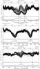 |
Fig. 5 Representative wind profiles from IUE spectra showing the typical variation over a 12-day cycle, which is very similar to the type of variation observed in other magnetic B stars but unlike the variations observed in O stars. Top: C iv. Middle: Si iv. Bottom: N v. The two doublet rest wavelengths are indicated by vertical dashed lines. Top scales: Wavelength. Bottom scales: velocity relative to the stellar rest frame. In each panel the lower part displays the significance of the variability, as the ratio of the measured to the expected variances. |
We used a superposition of two sine waves to fit the C iv EW data. The result is obtained with a least-squares method, which uses weights equal to 1/σ2 (with 1σ the individual error bars) assigned to each datapoint. With user-supplied initial starting values for the free parameters, a steepest descent technique then searched for the lowest minimum of the χ2. The variance matrix provides the formal errors in the parameters, as seen in the following function: f(t) = a + b(sin(2π(t/P + d))) + e(sin(2π(t/(P/2) + f))).
The results of the best solution with a reduced χ2 = 0.52
are: a = 2.41 ± 0.03, b = 0.60 ± 0.05,
d = 0.308 ± 0.009, e = 1.77 ± 0.04,
f = 0.84 ± 0.01, and a period P = 12.00075 ± 0.00011 d.
The very high precision of less than 10 s in the period is thanks to extended coverage
over almost 500 cycles. All doublet profiles of C iv, Si iv, and N v
are modulated with this same period, which is identified with the rotation period of
the star. With this analytic description, the epoch of minimum EW could be derived
mathematically. We derived the ephemeris for the deepest minimum (i.e. maximum emission),
which we define as the zero phase of the rotation. We find 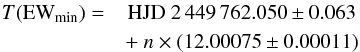 (3)with n defined as the number
of cycles. The reference date HJD 2 449 762.050 is at the EW minimum that is closest to
the middle of the IUE observations.
(3)with n defined as the number
of cycles. The reference date HJD 2 449 762.050 is at the EW minimum that is closest to
the middle of the IUE observations.
The phase difference between the maxima in the fitted EW curve is Δφmax = 0.527 ± 0.003, whereas the difference between the minima is Δφmin = 0.504 ± 0.002. The difference between these two values, and the unequal depths clearly indicates that the wind must be asymmetric with respect to the magnetic equator. For a banded oblique rotator (Shore 1987), the value of Δφ is directly related to the asymmetry in the magnetic modulation, which will be compared in Sect. 4.3.
4.2. Magnetic properties
A CLEAN analysis of all magnetic data reveals only one significant period of
P = 11.9971 ± 0.0078 d. This period is within the uncertainties equal
to the period derived from the much more accurate UV data. We therefore use the UV period
in our further analysis. We fitted a cosine function of the following form to the 130
Bℓ datapoints with
1/σ2 error bars as weights:
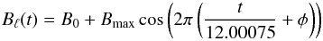 (4)in which t was taken
relative to the first observation. The best-fit values are B0
= −6 ± 3 G, Bmax = 97 ± 4 G, and
φ = 0.4759 ± 0.0079 with a reduced χ2 = 2.3.
(4)in which t was taken
relative to the first observation. The best-fit values are B0
= −6 ± 3 G, Bmax = 97 ± 4 G, and
φ = 0.4759 ± 0.0079 with a reduced χ2 = 2.3.
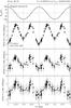 |
Fig. 6 Phase behaviour of the stellar wind lines and magnetic variation. Upper panel: best sinusoid fit to the magnetic data of β Cep as a function of the UV phase, using a fixed period of 12.00075 d, as derived from UV data. Two rotational periods are displayed. Vertical dashed lines at phases 0.5 and 1 serve as a reference for comparison with the stellar wind behaviour. Lower panels, respectively, from top to bottom: equivalent width of the C iv, Si iv, and N v stellar wind lines measured in IUE spectra taken during 16 years as a function of phase, which is calculated with Eq. (3). The deepest minimum, defined as phase 0, corresponds to the maximum emission, which occurs when the magnetic North pole is pointing most to the observer. Note that there is no significant difference in zero phase between the UV and magnetic data but that the field crosses zero slightly besides the EW maxima, as discussed in Sect. 4.3 |
With the derived phase, we find the maximum value of the field strength for the
ephemeris:  (5)The reference date HJD 2 452 366.25 is given
at the maximum field closest to the middle of the magnetic measurements, which extend over
200 cycles.
(5)The reference date HJD 2 452 366.25 is given
at the maximum field closest to the middle of the magnetic measurements, which extend over
200 cycles.
When omitting the 21 data points of the 2000 dataset because of the potential fringing problem mentioned above, we obtain B0 = −11 ± 3 G, Bmax = 101 ± 4 G, φ = 0.4913 ± 0.0077 with a reduced χ2 = 2.1, and a reference date of HJD 2 452 366.18 ± 0.09, which is hardly different from the fit with all data. Given the very small differences, we consider the fit above with all 130 datapoints still as the best.
In Fig. 4, we have drawn a sine wave with this period and phase through the early magnetic measurements of December 1998 until July 1999. Figures 6 and 7 show all 130 datapoints folded with the rotational period and an overplot of the best-fit cosine curve. In Fig. 7, the residuals from the fit are displayed. No obvious discrepancies are emerging with the limited accuracy of the present data.
4.3. Comparison between magnetic and wind properties
A comparison to the phase of the UV data (Eq. (3)) shows that a deep EW minimum is predicted at HJD 2 452 366.21 ± 0.04, which is, within the uncertainties, identical to the phase of maximum (positive) magnetic field. In Fig. 6 (2nd panel), we have drawn a sine wave with the best fit parameters through the values of the magnetic field strength and using the phase from the UV period. It is clear from the figure that the phase of minima of the stellar wind absorption (i.e. maximum emission) coincides very well with the extremes of the magnetic field, and that the maximum wind absorption coincides with a field strength zero. This is compatible with an oblique rotator model in which the wind outflow is much enhanced in the plane of the magnetic equator. It is of interest to note that the result of B0 = −6 ± 3 G implies that the asymmetry relative to zero must be small, although the shallower second EW minimum implies an asymmetric wind. This can be used to put constraints on the geometry of the field. As outlined by Shore (1987), the ratio of the extremes of the magnetic modulation r = Bmax/Bmin is related to the phase difference Δφ between the maxima or minima of the EW modulation by r = (u − 1)/(u + 1) with u = cos(Δφ/2). The values for Δφ in the previous section imply that B0 = 8.0 ± 1.2 G when de maxima are used, and that B0 = 0.6 ± 0.7 G when the minima are considered. A geometry that is compatible with the phase difference between the minima in the EW (with maximum positive field value) is therefore slightly favored. It is clear, however, that more magnetic data are needed to confirm any asymmetry.
For a dipolar field, the ratio r = Bmin/Bmax is also related to the inclination angle, i, and the angle of the magnetic axis relative to the rotation axis, β, according to r = cos(β + i)/cos(β − i) (Preston 1967). We obtain r = −1.12 ± 0.01, which can put further constraints upon the angles β and i. For i near 60°, it follows that β close to 96°. With a projected rotational velocity of 27(3) km s-1 (as derived by Telting et al. (1997) from a pulsation mode analysis), the rotation period requires a radius of 7.4 ± 0.8 R⊙, which is in excellent agreement with the value 7.5 ± 0.7 R⊙ that is based on Remie & Lamers (1982). These authors derived the angular size from the integrated total flux and infrared flux. A further discussion of the stellar parameters and the best-fit results of the angles i and β based on line fits to I and V is given by Donati et al. (2001).
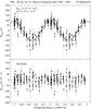 |
Fig. 7 Top: overplot of all magnetic data folded with the rotational period of 12.00075 d. Two rotational periods are displayed. The drawn curve is the best-fit cosine with amplitude 97 G and offset −6 G. Bottom: overplot of residuals (O−C) of all magnetic data folded with the rotational period. |
4.4. Pulsation period and system velocity
The measured radial velocities of the star are given in Col. 9 in Table 2. For the calculation of the phase in heliocentric radial velocity due to the radial mode of the pulsation, we used the ephemeris for the expected maximum from Pigulski & Boratyn (1992) with P = 0.1904852 d and Tmax = 2413499.5407 (Col. 7 in Table 2).
In Fig. 8, we plotted the derived radial velocity with the magnetic field strength as a function of the calculated pulsation phase for the first 23 measurements, which covered 7 months in 1998 and 1999. Taking all the data together would not make sense because of the expected systemic velocity of the star in its 90-year orbit, especially since the star was very near its periastron passage (see below). From the figure, it is clear that there is no correlation between the pulsation phase and the longitudinal component of the magnetic field, as expected. The correlation coefficient for a sine curve is only 0.11.
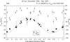 |
Fig. 8 Derived radial velocity (filled symbols, scale on the left) and magnetic field strength (open symbols, scale on the right) as a function of pulsation phase. As expected, no correlation between the two quantities is present in the data: at several occasions very different magnetic values are measured at a given pulsation phase. The observed system velocity and the difference between the observed and calculated phase of the maximum radial velocity confirm the predicted values for the star in its binary orbit near periastron passage. |
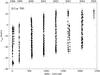 |
Fig. 9 Radial velocities as measured from all spectra from 1998–2005. |
Each magnetic measurement consists of four subexposures for each of which we determined
the radial velocity. (Only the average value per 4 subexposures is given in Table 2.) We also included spectra from incomplete sets,
which made a total of 477 data points, as shown in Fig. 9. We divided this dataset into logical subsets, with a coverage of about 0.5 to
3 weeks each year (see Col. 3 in Table 4) and
performed cosine fits for each subset with the function:  (6)The ephemeris and the period
P from Pigulski & Boratyn
(1992) were used to derive the phase φ and the delay of the
maximum of the radial velocity curve of the pulsation (O−C), which is attributed to the
light time effect. The results are given in Table 4. A best fit through the values of the system velocity γ of
Table 4 yielded the orbital parameters listed in
Table 5. We kept T0,
the passage of periastron, constant in this fit. Our orbital parameters agree fairly well
with those derived by Pigulski & Boratyn
(1992). With only 7 data points and 5 free parameters the error bars are expectedly
large for some of the parameters. We note that ω becomes 198° ± 2° if all
other values are kept constant, and that the error bar is derived by letting
χ2 increase by unity. Our values of the delays are also in
good agreement with the expected phase delay, which is caused by the light-time effect in
the binary orbit (see Pigulski & Boratyn
1992,their Fig. 1).
(6)The ephemeris and the period
P from Pigulski & Boratyn
(1992) were used to derive the phase φ and the delay of the
maximum of the radial velocity curve of the pulsation (O−C), which is attributed to the
light time effect. The results are given in Table 4. A best fit through the values of the system velocity γ of
Table 4 yielded the orbital parameters listed in
Table 5. We kept T0,
the passage of periastron, constant in this fit. Our orbital parameters agree fairly well
with those derived by Pigulski & Boratyn
(1992). With only 7 data points and 5 free parameters the error bars are expectedly
large for some of the parameters. We note that ω becomes 198° ± 2° if all
other values are kept constant, and that the error bar is derived by letting
χ2 increase by unity. Our values of the delays are also in
good agreement with the expected phase delay, which is caused by the light-time effect in
the binary orbit (see Pigulski & Boratyn
1992,their Fig. 1).
New orbital parameters with 1σ errors for the β Cep system, which is based on radial velocity measurements in this paper.
In the binary system, the companion has been resolved by interferometry. New speckle interferometric measurements by Balega et al. (2002) yielded a separation of 38 ± 2 mas at the epoch 1998.770 (i.e. just preceding our first observation) at a position angle of 228.6°, whereas the position angle was 49.3° (Hartkopf et al. 1992) with separation 50 mas 8 years earlier. This shows that the companion had passed a minimum radial velocity before our first observation. The binary period is therefore likely a little shorter than 85 years, based on the previous periastron passage in 1914.6 ± 0.4. This agrees with Hadrava & Harmanec (1996), who concluded that the periastron passage should be closer to 1996 than to 2006, as predicted by Pigulski & Boratyn (1992). Our orbital solution points to the same conclusion. A more accurate solution was achieved by Andrade (2006) with a new analysis, based on all available interferometric measurements between 1971.48 and 1998.77, which included the periastron passage. These results, given in Col. 3 Table 4, are in very good agreement of the findings of this paper.
5. Conclusions and discussion
We have unambiguously found a varying weak magnetic field in β Cep, which is consistent with an oblique dipolar magnetic rotator model with a rotation period of 12 days. Contrary to what is found in models by Brown et al. (1985), Shore (1987), and Shore et al. (1987), the UV wind-line absorption in β Cep is at a maximum if the Earth is in the magnetic equatorial plane. Model MHD calculations of the outflow and the resulting UV wind lines with a SEI-based code that were applied to β Cep are presented by Schnerr et al. (2007). They found that the observed variability of the wind lines could be qualitatively reproduced for simple phenomenological models with enhanced density in the magnetic equator (presumably due to magnetic channeling of the wind). However, significant differences are encountered when full 2D-MHD models were used to determine the geometry of the stellar wind. The authors ascribe this effect to X-ray ionisation that has not been included.
We emphasize that we have only measured the longitudinal component of the magnetic field, (i.e., the component in the line of sight, which is taken averaged over the stellar disk). The intensity at the magnetic poles must be stronger. For a perpendicular magnetic rotator the polar field of a dipole is 3.2 × Bℓ,max (Schwarzschild 1950), or about 300 G. However, the EW curve in the stellar wind lines has two unequal maxima at epochs when the projected field is strongest, which suggests that there should be a slight asymmetry present. This could of course be due to a slightly different geometry (off-centred dipole or higher-order fields) at the two hemispheres, which can easily be hidden in the observed field strength that is the integrated value over the visible surface. The EW maxima of the UV wind lines occur slightly off the phases 0.25 and 0.75, when the magnetic values cross zero, which also indicates some asymmetry.
We note that ths configuration found here favors magnetic braking as discussed by Donati et al. (2001), although the origin of the present slow rotation rate remained unclear. They calculated the characteristic spindown time to be 110 My for a mass-loss rate of 2.7 × 10⁻¹⁰M⊙ y-1 at an Alfvén radius of 9 R∗, which is about an order of magnitude longer than the age of the star. Applying the work by Ud-Doula et al. (2008) to β Cep gives a similar result. However, this may be an upper limit, as their model is applied to a pure dipole field aligned with the rotation axis, unlike the configuration in β Cep, which is an oblique rotator. We also must consider the possibility, as mentioned above, that the field is not dipole-like but resembles a split monopole, in which case the estimated spindown time can be as much as two orders of magnitudes shorter, which is of the order of 1 My (i.e., clearly within the lifetime of the star Ud-Doula et al. 2009).
It is also interesting to note that the mode splitting due to the rotation is clearly present in the pulsation properties (Telting et al. 1997). It would be worth examining whether the presence of the magnetic field can also be traced back in the pulsation modes. If so, this will give a strong constraint on the evolutionary status of β Cep. In this regard, it is clear that the analysis as presented by Shibahashi & Aerts (2000) should be revised, as it was based on a rotational period of 6 days rather than 12 days.
The X-ray flux of β Cep was detected by the Einstein Observatory (Grillo et al. 1992) and later by the ROSAT satellite Berghöfer et al. (1996). After the discovery of the magnetic field, the (static) magnetically confined shock (MWCS) model by Babel & Montmerle (1997) was used by Donati et al. (2001) to make specific predictions of the X-ray behaviour as a function of rotational phase. Dynamical modelling of the interaction of the wind and the magnetic field by ud-Doula & Owocki (2002), Gagné et al. (2005) and Townsend et al. (2005) showed, however, that an optically thick cool disk, as predicted by the MWCS model, would not form around β Cep. The lack of the predicted rotational modulation in the flux measured with the Chandra and XMM/Newton observatories analysed by Favata et al. (2009) confirmed the absence of such a static disk. The analysis of line ratios in the X-ray spectra allowed these authors to put constraints on the distance from the star where the relatively low-temperature X-ray plasma is confined, which is typically a few stellar radii, with a stratified temperature distribution. They also discuss the significant differences in X-ray and wind-confinement properties between β Cep and the more massive magnetic O4 star θ1 Ori C, for which the MWCS model is compatible with the observed X-ray characteristics.
The close environment of β Cep was recently investigated with interferometry by Nardetto et al. (2011) with a spatial resolution of 1 mas. They concluded that a circular ring (instead of a uniform disk) gives the best fit with a geometry and orientation similar to the magnetic equator, as described above, which is a remarkable result. They determined this result from model fits of the resolved large-scale structure around the star at two different rotational phases (0.47 and 0.17 with our ephemeris, which is about 0.03 lower than used in their paper). Their favored geometry gives an inner ring diameter of about 74 R∗, a width of 5 R∗, and a position angle of 60°. As discussed by these authors, this ring should be optically thin in the X-ray band and is also consistent with the absence of X-ray modulation reported by Favata et al. (2009). The radius of this ring is, however, larger than the region constrained by Favata et al. (2009).
Several other issues are still to be solved. First of all, why does β Cep have a magnetic field? This star does not belong to the helium-peculiar stars (Rachkovskaya 1990), which are known to have strong magnetic fields (see for instance Bohlender et al. 1987). We did not find any variability in the wind-sensitive He i 1640 line, although not much can be expected to show up in this very weak line with the very poor S/N (<10 in this wavelength region). Gies & Lambert (1992) note that β Cep is N enriched, a property that this star shares with other magnetic B stars, as confirmed by Morel et al. (2006) and Nieva & Przybilla (2012). Enrichment of nitrogen in the atmosphere of a B star is apparently a strong indirect indicator of a surface magnetic field (Henrichs et al. 2005). The presence of a magnetic field could cause these anomalies by inhibiting mixing in the interior, but no specific models have been developed to explain the N enrichment. Theoretical predictions for the nitrogen enrichment at the surface of B stars that host a large-scale, dipolar field have been presented by Meynet et al. (2011). Nieva & Przybilla (2012) considered the overabundance of nitrogen as a result of mixing of CN-recycled material into the stellar atmosphere. Wade et al. (2007) proposed a simple mechanism for why some A and B stars have magnetic fields.
Another point of concern is that we have fitted a simple sine curve through the magnetic data. This is obviously a first approximation, and when more accurate measurements become available, a search for deviations from a sine curve, as is found for most magnetic stars, can be done.
Lastly, one may wonder whether other pulsating B stars may show the same type of wind variability, which is specific for magnetic stars. An elaborated search by Henrichs and ten Kulve (in preparation) in the complete sample of IUE spectra of 395 B stars provided the best possible statistics to date. None of these stars (besides the well known magnetic Bp stars) except for β Cep, V2052 Oph (Neiner et al. 2003b; Briquet et al. 2012), ζ Cas (Neiner et al. 2003a), and the possibility of σ Lup (Henrichs et al. 2012) showed a similar periodic pattern. This must be regarded as a lower limit, since only very limited timeseries with poor coverage exist in most cases, which makes it impossible to quantify the real occurrence. Hubrig et al. (2011) searched in a number of pulsating B stars for magnetic fields. Silvester et al. (2009) concluded from a study of 30 stars that magnetism is not common among pulsating B stars. Recently, Petit et al. (2013) discussed the magnetic environments of all discovered massive magnetic stars, among which β Cep does magnetically not stand out. The star β Cep hence appears to be one of the very few stars in its class that shows the type of strong wind variability described here. In this respect β Cep is an exceptional β Cephei star.
Online material
Observations and results of magnetic measurements from MuSiCoS spectropolarimetry of β Cep at TBL at the Pic du Midi, 1998–2005.
Acknowledgments
We thank D. Lennon, G. Mathys, S. Solanki, J. Telting, and A. ud-Doula for discussions and constructive comments. We also thanks an anonymous referee for useful remarks and comments. H.F.H. thanks his coauthors for their patience and S. Hubrig for encouragement to finish this work. The helpful assistance and support of the observatory staff members at TBL, GSFC, and Vilspa (in particular, the late Dr. Willem Wamsteker) is well remembered and fondly acknowledged. J.D.J. acknowledges support from the Netherlands Foundation for Research in Astronomy (NFRA) with financial aid from the Netherlands Organization for Scientific Research (NWO) under project 781-71-053. G.A.W. acknowledges support from the Natural Sciences and Engineering Council of Canada (NSERC).
References
- Abt, H. A., Levato, H., & Grosso, M. 2002, ApJ, 573, 359 [NASA ADS] [CrossRef] [Google Scholar]
- Andrade, M. 2006, IAU Inf. Circ. Comm. 26, 158, 3 [Google Scholar]
- Babel, J., & Montmerle, T. 1997, A&A, 323, 121 [NASA ADS] [Google Scholar]
- Balega, I. I., Balega, Y. Y., Hofmann, K.-H., et al. 2002, A&A, 385, 87 [NASA ADS] [CrossRef] [EDP Sciences] [Google Scholar]
- Barker, P. K., Brown, D. N., Bolton, C. T., & Landstreet, J. D. 1982, in Advances in Ultraviolet Astronomy, ed. Y. Kondo, 589 [Google Scholar]
- Baudrand, J., & Bohm, T. 1992, A&A, 259, 711 [NASA ADS] [Google Scholar]
- Berghöfer, T. W., Schmitt, J. H. M. M., & Cassinelli, J. P. 1996, A&AS, 118, 481 [NASA ADS] [CrossRef] [EDP Sciences] [Google Scholar]
- Bohlender, D. A., Landstreet, J. D., Brown, D. N., & Thompson, I. B. 1987, ApJ, 323, 325 [NASA ADS] [CrossRef] [Google Scholar]
- Briquet, M., Neiner, C., Aerts, C., et al. 2012, MNRAS, 427, 483 [NASA ADS] [CrossRef] [Google Scholar]
- Brown, D. N., Shore, S. N., & Sonneborn, G. 1985, AJ, 90, 1354 [NASA ADS] [CrossRef] [Google Scholar]
- Catala, C., Foing, B. H., Baudrand, J., et al. 1993, A&A, 275, 245 [NASA ADS] [Google Scholar]
- Chalabaev, A., & Maillard, J. P. 1983, A&A, 127, 279 [NASA ADS] [Google Scholar]
- Donati, J.-F., Semel, M., Carter, B. D., Rees, D. E., & Collier Cameron, A. 1997, MNRAS, 291, 658 [NASA ADS] [CrossRef] [MathSciNet] [Google Scholar]
- Donati, J.-F., Catala, C., Wade, G. A., et al. 1999, A&AS, 134, 149 [NASA ADS] [CrossRef] [EDP Sciences] [Google Scholar]
- Donati, J.-F., Wade, G. A., Babel, J., et al. 2001, MNRAS, 326, 1265 [NASA ADS] [CrossRef] [Google Scholar]
- Favata, F., Neiner, C., Testa, P., Hussain, G., & Sanz-Forcada, J. 2009, A&A, 495, 217 [NASA ADS] [CrossRef] [EDP Sciences] [Google Scholar]
- Fischel, D., & Sparks, W. M. 1972, in The scientifique results from the Orbiting Astronomical Observatory (OAO-2), NASA SP-310, 475 [Google Scholar]
- Frost, E. B., & Adams, W. S. 1903, ApJ, 17, 150 [NASA ADS] [CrossRef] [Google Scholar]
- Gagné, M., Oksala, M. E., Cohen, D. H., et al. 2005, ApJ, 628, 986 [NASA ADS] [CrossRef] [Google Scholar]
- Gezari, D. Y., Labeyrie, A., & Stachnik, R. V. 1972, ApJ, 173, L1 [NASA ADS] [CrossRef] [Google Scholar]
- Gies, D. R., & Lambert, D. L. 1992, ApJ, 387, 673 [NASA ADS] [CrossRef] [Google Scholar]
- Grillo, F., Sciortino, S., Micela, G., Vaiana, G. S., & Harnden, F. R. Jr., 1992, ApJS, 81, 795 [NASA ADS] [CrossRef] [Google Scholar]
- Hadrava, P., & Harmanec, P. 1996, A&A, 315, L401 [NASA ADS] [Google Scholar]
- Hartkopf, W. I., McAlister, H. A., & Franz, O. G. 1992, AJ, 104, 810 [NASA ADS] [CrossRef] [Google Scholar]
- Henrichs, H. F., Bauer, F., Hill, G. M., et al. 1993, in IAU Colloq. 139: New Perspectives on Stellar Pulsation and Pulsating Variable Stars, eds. J. M. Nemec & J. M. Matthews, 186 [Google Scholar]
- Henrichs, H. F., Kaper, L., & Nichols, J. S. 1994, A&A, 285, 565 [NASA ADS] [Google Scholar]
- Henrichs, H. F., de Jong, J. A., Nichols, J. S., et al. 1998, in Ultraviolet Astrophysics Beyond the IUE Final Archive, eds. W. Wamsteker, R. Gonzalez Riestra, & B. Harris, ESA SP, 413, 157 [Google Scholar]
- Henrichs, H. F., Schnerr, R. S., & Ten Kulve, E. 2005, in The Nature and Evolution of Disks Around Hot Stars, ASP Conf. Ser., 337, 114 [NASA ADS] [Google Scholar]
- Henrichs, H. F., Kolenberg, K., Plaggenborg, B., et al. 2012, A&A, 545, A119 [NASA ADS] [CrossRef] [EDP Sciences] [Google Scholar]
- Heynderickx, D., Waelkens, C., & Smeyers, P. 1994, A&AS, 105, 447 [NASA ADS] [Google Scholar]
- Hubrig, S., Ilyin, I., Schöller, M., et al. 2011, ApJ, 726, L5 [NASA ADS] [CrossRef] [Google Scholar]
- Kaper, L., & Mathias, P. 1995, in IAU Colloq. 155: Astrophysical Applications of Stellar Pulsation, eds. R. S. Stobie, & P. A. Whitelock, ASP Conf. Ser., 83, 295 [Google Scholar]
- Kaper, L., Henrichs, H. F., & Mathias, P. 1992, Decline in the Halpha emission strength of beta Cephei, OHP Newsletter, February [Google Scholar]
- Kaper, L., Henrichs, H. F., Nichols, J. S., et al. 1996, A&AS, 116, 257 [NASA ADS] [CrossRef] [EDP Sciences] [Google Scholar]
- Landstreet, J. D. 1982, ApJ, 258, 639 [NASA ADS] [CrossRef] [Google Scholar]
- Lesh, J. R. 1968, ApJS, 17, 371 [NASA ADS] [CrossRef] [EDP Sciences] [Google Scholar]
- Mathias, P., Gillet, D., & Kaper, L. 1991, in Rapid Variability of OB-stars: Nature and Diagnostic Value, ed. D. Baade, 193 [Google Scholar]
- Mathys, G. 1989, Fundamentals of Cosmic Physics, 13, 143 [NASA ADS] [Google Scholar]
- Meynet, G., Eggenberger, P., & Maeder, A. 2011, A&A, 525, L11 [NASA ADS] [CrossRef] [EDP Sciences] [Google Scholar]
- Morel, T., Butler, K., Aerts, C., Neiner, C., & Briquet, M. 2006, A&A, 457, 651 [NASA ADS] [CrossRef] [EDP Sciences] [Google Scholar]
- Nardetto, N., Mourard, D., Tallon-Bosc, I., et al. 2011, A&A, 525, A67 [NASA ADS] [CrossRef] [EDP Sciences] [Google Scholar]
- Neiner, C., Geers, V. C., Henrichs, H. F., et al. 2003a, A&A, 406, 1019 [NASA ADS] [CrossRef] [EDP Sciences] [Google Scholar]
- Neiner, C., Hubert, A.-M., Frémat, Y., et al. 2003b, A&A, 409, 275 [NASA ADS] [CrossRef] [EDP Sciences] [Google Scholar]
- Nieva, M.-F., & Przybilla, N. 2012, A&A, 539, A143 [NASA ADS] [CrossRef] [EDP Sciences] [Google Scholar]
- Panek, R. J., & Savage, B. D. 1976, ApJ, 206, 167 [NASA ADS] [CrossRef] [Google Scholar]
- Pan’ko, E. A., & Tarasov, A. E. 1997, Astron. Lett., 23, 545 [NASA ADS] [Google Scholar]
- Petit, V., Owocki, S. P., Wade, G. A., et al. 2013, MNRAS, 429, 398 [NASA ADS] [CrossRef] [Google Scholar]
- Pigulski, A., & Boratyn, D. A. 1992, A&A, 253, 178 [NASA ADS] [Google Scholar]
- Preston, G. W. 1967, ApJ, 150, 547 [NASA ADS] [CrossRef] [Google Scholar]
- Rachkovskaya, T. M. 1990, Bull. Crimean Astrophys. Obs., 82, 1 [NASA ADS] [Google Scholar]
- Remie, H., & Lamers, H. J. G. L. M. 1982, A&A, 105, 85 [Google Scholar]
- Rudy, R. J., & Kemp, J. C. 1978, MNRAS, 183, 595 [NASA ADS] [CrossRef] [Google Scholar]
- Schnerr, R. S., Henrichs, H. F., Oudmaijer, R. D., & Telting, J. H. 2006a, A&A, 459, L21 [NASA ADS] [CrossRef] [EDP Sciences] [Google Scholar]
- Schnerr, R. S., Verdugo, E., Henrichs, H. F., & Neiner, C. 2006b, A&A, 452, 969 [NASA ADS] [CrossRef] [EDP Sciences] [Google Scholar]
- Schnerr, R. S., Henrichs, H. F., Owocki, S. P., Ud-Doula, A., & Townsend, R. H. D. 2007, in Active OB-Stars: Laboratories for Stellare and Circumstellar Physics, eds. A. T. Okazaki, S. P. Owocki, & S. Stefl, ASP Conf. Ser., 361, 488 [Google Scholar]
- Schrijvers, C., Telting, J. H., Aerts, C., Ruymaekers, E., & Henrichs, H. F. 1997, A&AS, 121, 343 [NASA ADS] [CrossRef] [EDP Sciences] [Google Scholar]
- Schwarzschild, M. 1950, ApJ, 112, 222 [NASA ADS] [CrossRef] [Google Scholar]
- Shibahashi, H., & Aerts, C. 2000, ApJ, 531, L143 [NASA ADS] [CrossRef] [Google Scholar]
- Shore, S. N. 1987, AJ, 94, 731 [NASA ADS] [CrossRef] [Google Scholar]
- Shore, S. N., Brown, D. N., & Sonneborn, G. 1987, AJ, 94, 737 [NASA ADS] [CrossRef] [Google Scholar]
- Silvester, J., Neiner, C., Henrichs, H. F., et al. 2009, MNRAS, 398, 1505 [NASA ADS] [CrossRef] [Google Scholar]
- Telting, J. H., Aerts, C., & Mathias, P. 1997, A&A, 322, 493 [NASA ADS] [Google Scholar]
- Townsend, R. H. D., Owocki, S. P., & Groote, D. 2005, ApJ, 630, L81 [NASA ADS] [CrossRef] [Google Scholar]
- ud-Doula, A., & Owocki, S. P. 2002, ApJ, 576, 413 [NASA ADS] [CrossRef] [Google Scholar]
- Ud-Doula, A., Owocki, S. P., & Townsend, R. H. D. 2008, MNRAS, 385, 97 [NASA ADS] [CrossRef] [Google Scholar]
- Ud-Doula, A., Owocki, S. P., & Townsend, R. H. D. 2009, MNRAS, 392, 1022 [NASA ADS] [CrossRef] [Google Scholar]
- van Leeuwen, F. 2007, A&A, 474 [Google Scholar]
- Wade, G. A., Bohlender, D. A., Brown, D. N., et al. 1997, A&A, 320, 172 [NASA ADS] [Google Scholar]
- Wade, G. A., Donati, J.-F., Landstreet, J. D., & Shorlin, S. L. S. 2000, MNRAS, 313, 851 [NASA ADS] [CrossRef] [Google Scholar]
- Wade, G. A., Aurière, M., Bagnulo, S., et al. 2006, A&A, 451, 293 [NASA ADS] [CrossRef] [EDP Sciences] [Google Scholar]
- Wade, G. A., Silvester, J., Bale, K., et al. 2007 [arXiv:0712.3614] [Google Scholar]
- Wheelwright, H. E., Oudmaijer, R. D., & Schnerr, R. S. 2009, A&A, 497, 487 [NASA ADS] [CrossRef] [EDP Sciences] [Google Scholar]
All Tables
Illustrative sample calculations of magnetic-field strength without and with fringe correction and with different selections of spectral lines and weights (line depths) used for the construction of the LSD Stokes V profile.
New orbital parameters with 1σ errors for the β Cep system, which is based on radial velocity measurements in this paper.
Observations and results of magnetic measurements from MuSiCoS spectropolarimetry of β Cep at TBL at the Pic du Midi, 1998–2005.
All Figures
|
Fig. 1 Early magnetic measurements of β Cep, which are obtained with the University of Western Ontario photoelectric Pockels cell polarimeter and 1.2m telescope. Typical exposure times were between 1 and 3.5 h. The dashed curve is the best sinusoid fit, based on the analysis of all data points in this paper, and is the same as in Fig. 6. |
| In the text | |
|
Fig. 2 Top: overplot of a smoothed Stokes V spectrum of Vega (dashed line) and a Stokes V spectrum of β Cep (1999, nr. 22). Both contain a strong spurious modulation caused by fringing on the CCD. Bottom: Stokes V spectrum of β Cep after removal of the fringes. |
| In the text | |
|
Fig. 3 Representative LSD Stokes unpolarised I (lower panel) and circularly polarised V (upper panel) profiles of β Cep from top to bottom on 15 and 18 December 1998, 15 January, and 3 July 1999. The signal- to-noise ratio (S/N) per velocity bin in the raw data is indicated. Note the clear Zeeman signatures at the zero, positive, and negative fields. The two lower figures illustrate negative fields at almost opposite pulsation phases. In Sect. 4, we show that the pulsation phase does not affect the magnetic field determination. |
| In the text | |
|
Fig. 4 The discovery observations, which include the first 23 datapoints from December 1998 until July 1999. The longitudinal component of the averaged surface magnetic field of β Cep is plotted. The dashed curve is the best-fit sine curve for all magnetic data with a fixed period of 12.00075 d, as derived from UV data. |
| In the text | |
|
Fig. 5 Representative wind profiles from IUE spectra showing the typical variation over a 12-day cycle, which is very similar to the type of variation observed in other magnetic B stars but unlike the variations observed in O stars. Top: C iv. Middle: Si iv. Bottom: N v. The two doublet rest wavelengths are indicated by vertical dashed lines. Top scales: Wavelength. Bottom scales: velocity relative to the stellar rest frame. In each panel the lower part displays the significance of the variability, as the ratio of the measured to the expected variances. |
| In the text | |
|
Fig. 6 Phase behaviour of the stellar wind lines and magnetic variation. Upper panel: best sinusoid fit to the magnetic data of β Cep as a function of the UV phase, using a fixed period of 12.00075 d, as derived from UV data. Two rotational periods are displayed. Vertical dashed lines at phases 0.5 and 1 serve as a reference for comparison with the stellar wind behaviour. Lower panels, respectively, from top to bottom: equivalent width of the C iv, Si iv, and N v stellar wind lines measured in IUE spectra taken during 16 years as a function of phase, which is calculated with Eq. (3). The deepest minimum, defined as phase 0, corresponds to the maximum emission, which occurs when the magnetic North pole is pointing most to the observer. Note that there is no significant difference in zero phase between the UV and magnetic data but that the field crosses zero slightly besides the EW maxima, as discussed in Sect. 4.3 |
| In the text | |
|
Fig. 7 Top: overplot of all magnetic data folded with the rotational period of 12.00075 d. Two rotational periods are displayed. The drawn curve is the best-fit cosine with amplitude 97 G and offset −6 G. Bottom: overplot of residuals (O−C) of all magnetic data folded with the rotational period. |
| In the text | |
|
Fig. 8 Derived radial velocity (filled symbols, scale on the left) and magnetic field strength (open symbols, scale on the right) as a function of pulsation phase. As expected, no correlation between the two quantities is present in the data: at several occasions very different magnetic values are measured at a given pulsation phase. The observed system velocity and the difference between the observed and calculated phase of the maximum radial velocity confirm the predicted values for the star in its binary orbit near periastron passage. |
| In the text | |
|
Fig. 9 Radial velocities as measured from all spectra from 1998–2005. |
| In the text | |
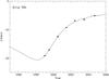 |
Fig. 10 Observed system velocity γ overplotted with the orbital solution from Table 5. |
| In the text | |
Current usage metrics show cumulative count of Article Views (full-text article views including HTML views, PDF and ePub downloads, according to the available data) and Abstracts Views on Vision4Press platform.
Data correspond to usage on the plateform after 2015. The current usage metrics is available 48-96 hours after online publication and is updated daily on week days.
Initial download of the metrics may take a while.