| Issue |
A&A
Volume 555, July 2013
|
|
|---|---|---|
| Article Number | A37 | |
| Number of page(s) | 10 | |
| Section | Cosmology (including clusters of galaxies) | |
| DOI | https://doi.org/10.1051/0004-6361/201321048 | |
| Published online | 26 June 2013 | |
Full-sky CMB lensing reconstruction in presence of sky-cuts
1
Department of Physics and AstronomyUniversity College London,
London
WC1E 6BT,
UK
e-mail:
This email address is being protected from spambots. You need JavaScript enabled to view it.
2
Institut d’Astrophysique de Paris, CNRS, UMR 7095, Université
Pierre & Marie Curie, 98bis boulevard Arago, 75014
Paris,
France
3
Astroparticule et Cosmologie, CNRS UMR 7164, Université Denis
Diderot Paris 7, Bâtiment
Condorcet, 10 rue A. Domon et L. Duquet, 75013
Paris,
France
4
Laboratoire Traitement et de l’Information, CNRS UMR 5141 and
Télécom ParisTech, 46 rue
Barrault, 75634
Paris Cedex 13,
France
5
Jet Propulsion Laboratory, California Institute of Technology,
4800 Oak Grove
Drive, Pasadena,
CA
91109,
USA
6
Departement of Physics, McGill University,
Montreal, QC
H3A 2T8,
Canada
Received:
6
January
2013
Accepted:
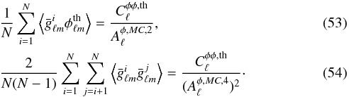
13
March
2013
Abstract
We consider the reconstruction of the CMB lensing potential and its power spectrum on the full sphere in presence of sky-cuts due to point sources and Galactic contamination. These two effects are treated separately. Small regions contaminated by point sources are filled in using constrained Gaussian realizations. The Galactic plane is simply removed using an apodized mask before lensing reconstruction. This algorithm recovers the power spectrum of the lensing potential with no significant bias.
Key words: gravitational lensing: weak / methods: data analysis / cosmic background radiation
© ESO, 2013
1. Introduction
Gravitational lensing by large scale structure generates a deflection of the trajectories
of the cosmic microwave background (CMB) photons. This effect, known as CMB lensing has long
been predicted (Blanchard & Schneider 1987;
Bernardeau 1998; Zaldarriaga & Seljak 1999; see Lewis
& Challinor 2006 for a review). It was first detected by cross-correlating
CMB data with large-scale structure (Smith et al.
2007; Hirata et al. 2008) and was recently
detected internally using only CMB observations (Das et al.
2011; van Engelen et al. 2012). CMB lensing
consists in a remapping of the underlying unlensed temperature field. The lensed CMB is
related to the unlensed by the deflection angle d, which is the gradient of the
CMB lensing potential  (with
(with  ).
).
The lensing potential
is defined as the integral along the line of sight of the gravitational potential weighted
by a geometrical kernel 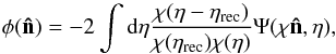 (1)where Ψ is the Newtonian
potential, η is the conformal time, ηrec is the
epoch of last scattering, and χ is the angular diameter distance in
comoving coordinates. The lensing potential thus contains valuable information on
large-scale structure and on the cosmological parameters governing their growth such as the
equation of state of dark energy or the sum of neutrino masses (Lesgourgues et al. 2006; Benoit-Lévy et
al. 2012). It is therefore of utmost importance to be able to recover the lensing
potential and its power spectrum from the wealth of high quality CMB data which will soon be
available, especially with the forthcoming data of the Planck satellite.
(1)where Ψ is the Newtonian
potential, η is the conformal time, ηrec is the
epoch of last scattering, and χ is the angular diameter distance in
comoving coordinates. The lensing potential thus contains valuable information on
large-scale structure and on the cosmological parameters governing their growth such as the
equation of state of dark energy or the sum of neutrino masses (Lesgourgues et al. 2006; Benoit-Lévy et
al. 2012). It is therefore of utmost importance to be able to recover the lensing
potential and its power spectrum from the wealth of high quality CMB data which will soon be
available, especially with the forthcoming data of the Planck satellite.
CMB lensing modifies the Gaussian structure of the primary anisotropies and generates a correlation between the temperature and its gradient (Hu 2000). These couplings can efficiently be used to construct an estimator, quadratic in the observed temperature, that can be applied to data to recover the lensing potential (Okamoto & Hu 2003).
Reconstruction of the lensing potential on the full sky requires specially designed techniques to account for the complications inherent to real-world data analysis. In particular, the presence of regions of the sky which are highly contaminated by Galactic emission or by point sources prevents the direct and straightforward use of the quadratic estimator. Various techniques have been developed to account for sky-cuts in a full sky CMB lensing analysis. Perotto et al. (2010) developed an algorithm to reconstruct the Gaussian fluctuations of the CMB inside the masked regions. Smith et al. (2007) chose to perform optimal filtering of the observed temperature, by inverting the full variance of the data. This expensive operation, which requires the inversion of a matrix (Npix × Npix) would be feasible at the Planck resolution but requires CPU consuming algorithms. Finally, Plaszczynski et al. (2012) recently proposed a hybrid method which decomposes the region outside the Galactic mask into small patches on which a flat-sky analysis can be performed.
Is this article, we present a new and simple method to reconstruct the lensing potential on the sphere. We treat differently the zones of the sky which must be removed because of the presence of point sources and the regions contaminated by the Galaxy. The pixels corresponding to point sources are inpainted with Gaussian constrained realizations. The idea is to restore isotropic Gaussian CMB fluctuations at the expense of adding a small amount of noise in the data, such that the lensing estimator has the same response as it would have in the ideal case. Regarding the Galactic cut, we choose to apodize the Galactic mask and perform the usual isotropic filtering required by the lensing estimator on the masked data. As we will show later, this operation is almost harmless to the lensing signal.
In Sect. 2, we present the formalism used in this paper for lensing reconstruction.
In Sect. 3 we investigate the question of the point sources mask, and in Sect. 4 we address the Galactic mask. Finally, in Sect. 5 we present a reconstruction where both issues are present.
2. Lensing reconstruction
We review in this section the formalism of CMB lensing and CMB lens reconstruction.
2.1. Notations
Throughout this paper, unlensed quantities are denoted with a tilde. Thus,
Cℓ denote the lensed TT power spectrum and
 ,
the unlensed. CMB lensing consists in a remapping of the unlensed temperature on the sky:
,
the unlensed. CMB lensing consists in a remapping of the unlensed temperature on the sky:
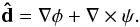
![Mathematical equation: \begin{equation} \theta\left[{\vec {\hat n}}\right] = \tilde \theta[{\vec {\hat n}} + {\vec {\hat d}}], \label{eq:cmblens1} \end{equation}](/articles/aa/full_html/2013/07/aa21048-13/aa21048-13-eq12.png) (2)where
(2)where
 is the deflection angle. This deflection angle can be expressed as the gradient of the
lensing potential φ, but for generality can also have a curl component
(Hirata & Seljak 2003; Namikawa et al. 2012)
is the deflection angle. This deflection angle can be expressed as the gradient of the
lensing potential φ, but for generality can also have a curl component
(Hirata & Seljak 2003; Namikawa et al. 2012)
 (3)At first-order,
in ΛCDM structure formation the deflection is a pure gradient and the curl component is
null (ψ = 0), although there exist other mechanisms which could lead to
non-zero curl in the deflection angle (e.g., primordial background of gravitational waves
from inflation Cooray et al. 2005, cosmic strings
Benabed & Bernardeau 2000). At higher
order, field rotation creates non-zero curl modes (Hirata
& Seljak 2003), but their amplitude are 10-3−10-2
smaller than the gradient modes (Lewis & Challinor
2006).
(3)At first-order,
in ΛCDM structure formation the deflection is a pure gradient and the curl component is
null (ψ = 0), although there exist other mechanisms which could lead to
non-zero curl in the deflection angle (e.g., primordial background of gravitational waves
from inflation Cooray et al. 2005, cosmic strings
Benabed & Bernardeau 2000). At higher
order, field rotation creates non-zero curl modes (Hirata
& Seljak 2003), but their amplitude are 10-3−10-2
smaller than the gradient modes (Lewis & Challinor
2006).
2.2. Quadratic estimator
The idea of lensing reconstruction is based upon the off-diagonal terms in the CMB
covariance that are created by CMB lensing. Lensing reconstruction then simply consists in
computing the correlations between a filtered version of the observed temperature with a
filtered version of its gradient (Okamoto & Hu
2003). The first step in the reconstruction consists of filtering the observed
temperature by its variance. This can be done in several ways, either by inverting the
full covariance matrix of the fluctuations (Smith et al.
2007), or more simply by applying an isotropic filtering. We choose the latter
option and our inverse filtered map then takes the following form
 (4)where
 are the
harmonic multipoles of the observed temperature, and
are the
harmonic multipoles of the observed temperature, and
 is the
total power spectrum of the observed temperature. This total spectrum can be decomposed as
is the
total power spectrum of the observed temperature. This total spectrum can be decomposed as
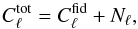 (5)where
 is a
fiducial lensed power spectrum and Nℓ is the
power spectrum of the instrumental noise, which is considered here as white and
homogeneous
is a
fiducial lensed power spectrum and Nℓ is the
power spectrum of the instrumental noise, which is considered here as white and
homogeneous 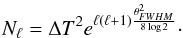 (6)Here ΔT
is the instrumental sensitivity and θFWVM is the angular
resolution parameter of the CMB experiment (Knox
1995).
(6)Here ΔT
is the instrumental sensitivity and θFWVM is the angular
resolution parameter of the CMB experiment (Knox
1995).
The inverse variance filtered multipoles are then used as an input to the quadratic
estimator. We follow the construction of the quadratic estimator by Okamoto & Hu (2003), but we slightly modify it along the lines
of Lewis et al. (2011). Instead of filtering the
observed map by the unlensed temperature power spectrum, we use the lensed power spectrum.
This small modification has been shown to greatly simplify the expression of the variance
of the lensing estimator (Hanson et al. 2011) –
hence the estimation of the lensing power spectrum. To summarize, we consider the
following fields  (7)with
 (8)We then consider
the product of θ(1) with the gradient of
θ(2),
θ(1)∇θ(2) (Hu 2000). This quantity is a vector field from which we can extract the
curl-free
(8)We then consider
the product of θ(1) with the gradient of
θ(2),
θ(1)∇θ(2) (Hu 2000). This quantity is a vector field from which we can extract the
curl-free  and gradient-free
  components. After calculations,
and
take the following forms:
components. After calculations,
and
take the following forms:  (9)and
 (10)where
 and
and
![Mathematical equation: \begin{equation} p^\pm_{\ell \ell1 \ell_2 }= \frac{\left[ 1 \pm(-1)^{\ell+\ell_1+\ell_2}\right] }{2}\cdot \end{equation}](/articles/aa/full_html/2013/07/aa21048-13/aa21048-13-eq38.png) (13)
and
are estimators of the lensing potential and the curl mode respectively. The expectation of
these two estimators are
(13)
and
are estimators of the lensing potential and the curl mode respectively. The expectation of
these two estimators are ![Mathematical equation: \begin{equation} \langle \bar{g}_{\ell m}\rangle = [A^{\phi}_\ell]^{-1} \phi_{\ell m} \label{meangrad} \end{equation}](/articles/aa/full_html/2013/07/aa21048-13/aa21048-13-eq39.png) (14)and
(14)and
 (15)where
 is a scalar
function that renormalizes the estimator so that the normalized estimator,
is a scalar
function that renormalizes the estimator so that the normalized estimator,
 , is unbiased
 (16)We can easily show
that takes the
following form
(16)We can easily show
that takes the
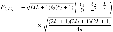
following form ![Mathematical equation: \begin{eqnarray} \left[A^{\phi}_\ell\right]^{-1}&=& -\frac{1}{4\pi}\sqrt{\ell(\ell+1)}\sum_{\ell_1 \ell_2} f_1(\ell_1) f_2(\ell_2)\nonumber\\ && \times (2\ell_1+1)(2\ell_2+1)\wj{\ell_1}{\ell_2}{\ell}{0}{-1}{1}\sqrt{\ell_2(\ell_2+1)}p^+_{\ell \ell_1 \ell_2} \nonumber\\ &&\times \left[ C_{\ell_1}\sqrt{\ell_1(\ell_1+1)}\wj{\ell_2}{\ell_1}{\ell}{0}{-1}{1} \right. \nonumber\\ &&+\left.C_{\ell_2}\sqrt{\ell_2(\ell_2+1)}\wj{\ell_1}{\ell_2}{\ell}{0}{-1}{1} \right]. \end{eqnarray}](/articles/aa/full_html/2013/07/aa21048-13/aa21048-13-eq44.png) (17)Operationally,
this quadratic estimator can easily be implemented using the HEALPix (Górski et al. 2005) routine map2alm_spin with the two
components of θ(1)∇θ(2) as an
input. It is worth noting that our estimator is written in a different way from that of
Okamoto & Hu (2003) and its expression
differs by a factor
(17)Operationally,
this quadratic estimator can easily be implemented using the HEALPix (Górski et al. 2005) routine map2alm_spin with the two
components of θ(1)∇θ(2) as an
input. It is worth noting that our estimator is written in a different way from that of
Okamoto & Hu (2003) and its expression
differs by a factor  .
This can be explained as Okamoto & Hu
(2003) considered the divergence of the temperature-gradient product
θ(1)∇θ(2) to extract the
curl-free part and then the lensing potential. Their estimator then involves an additional
derivative which explains the
factor.
.
This can be explained as Okamoto & Hu
(2003) considered the divergence of the temperature-gradient product
θ(1)∇θ(2) to extract the
curl-free part and then the lensing potential. Their estimator then involves an additional
derivative which explains the
factor.
The variance of the lensing potential estimator is given by (Okamoto & Hu 2003; Kesden et
al. 2003; Hanson et al. 2011)
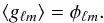
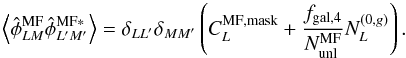
![Mathematical equation: \begin{equation} \left\langle g_{LM}g^*_{L^\prime M^\prime} \right\rangle= \delta_{LL^\prime}\delta_{MM^\prime}\left[C_L^{\phi\phi}+ N^{(0,g)}_L+ N^{(1,g)}_L\right] \end{equation}](/articles/aa/full_html/2013/07/aa21048-13/aa21048-13-eq46.png) (18)where
(18)where
 is a
bias term which emerges from the unlensed CMB. More precisely, the
is a
bias term which emerges from the unlensed CMB. More precisely, the
 bias is the response of the power spectrum of the quadratic estimator to the underlying
unlensed CMB which has a non-zero disconnected trispectrum (Hu 2001)
bias is the response of the power spectrum of the quadratic estimator to the underlying
unlensed CMB which has a non-zero disconnected trispectrum (Hu 2001) ![Mathematical equation: \begin{eqnarray} N^{(0,g)}_\ell&=&\frac{\left[A^{\phi}_\ell\right]^2}{4\pi} \sum_{\ell_1 \ell_2} f_1(\ell_1) f_2(\ell_2) \sqrt{\ell_2(\ell_2+1)} \\\nonumber &&\times (2\ell_1+1)(2\ell_2+1)\wj{\ell_1}{\ell_2}{\ell}{0}{-1}{1}C^{\rm{tot}}_{\ell_1}C^{\rm{tot}}_{\ell_2}p^+_{\ell \ell_1 \ell_2}\\\nonumber &&\times \left[ f_1(\ell_1) f_2(\ell_2) \sqrt{\ell_2(\ell_2+1)} \wj{\ell_1}{\ell_2}{\ell}{0}{-1}{1} \right.\\\nonumber &&+ \left.f_1(\ell_2) f_2(\ell_1) \sqrt{\ell_1(\ell_1+1)} \wj{\ell_2}{\ell_1}{\ell}{0}{-1}{1} \right]. \end{eqnarray}](/articles/aa/full_html/2013/07/aa21048-13/aa21048-13-eq49.png) (19)The
N(1,g) term can be expressed in the
full-sky formalism (Hanson et al. 2011), but we
need to resort to the flat-sky approximation (Kesden et
al. 2003) for a computable expression (Lesgourgues et al. 2005). Following Hanson et
al. (2011), N(1,g) takes the
following form
(19)The
N(1,g) term can be expressed in the
full-sky formalism (Hanson et al. 2011), but we
need to resort to the flat-sky approximation (Kesden et
al. 2003) for a computable expression (Lesgourgues et al. 2005). Following Hanson et
al. (2011), N(1,g) takes the
following form 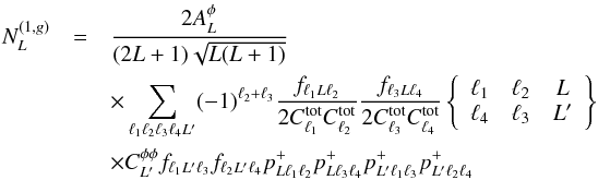 (20)with
 (21)and
 (22)This
expression for
Fℓ1Lℓ2
is more general than the one frequently used in the literature and is valid whatever is
the parity of the quantity
ℓ1 + ℓ2 + L.
(22)This
expression for
Fℓ1Lℓ2
is more general than the one frequently used in the literature and is valid whatever is
the parity of the quantity
ℓ1 + ℓ2 + L.
We also consider the variance of the estimator of the curl modes. Similarly, we have
![Mathematical equation: \begin{equation} \langle c_{LM}c^*_{L^\prime M^\prime} \rangle= \delta_{LL^\prime}\delta_{MM^\prime}\left[ N^{(0,c)}_L+ N^{(1,c)}_L\right], \end{equation}](/articles/aa/full_html/2013/07/aa21048-13/aa21048-13-eq56.png) (23)where
(23)where
 are
similar to
are
similar to  , the
only difference being in the parity conditions in their definitions
, the
only difference being in the parity conditions in their definitions ![Mathematical equation: \begin{eqnarray} N^{(0,c)}_\ell&=&\frac{[A^{\phi}_\ell]^2}{4\pi} \sum_{\ell_1 \ell_2} f_1(\ell_1) f_2(\ell_2) \sqrt{\ell_2(\ell_2+1)} \\\nonumber &&\times (2\ell_1+1)(2\ell_2+1)\wj{\ell_1}{\ell_2}{\ell}{0}{-1}{1}C^{\rm{tot}}_{\ell_1}C^{\rm{tot}}_{\ell_2}p^-_{\ell \ell_1 \ell_2}\\\nonumber &&\times \left[ f_1(\ell_1) f_2(\ell_2) \sqrt{\ell_2(\ell_2+1)} \wj{\ell_1}{\ell_2}{\ell}{0}{-1}{1} \right.\\\nonumber && + \left.f_1(\ell_2) f_2(\ell_1) \sqrt{\ell_1(\ell_1+1)} \wj{\ell_2}{\ell_1}{\ell}{0}{-1}{1} \right], \nonumber\\ \label{N1c} N^{(1,c)}_L&=& \frac{2A^{\phi}_L}{(2L+1)\sqrt{L(L+1)}}\\\nonumber &&\times \sum_{\ell_1 \ell_2 \ell_3 \ell_4 L^\prime}(-1)^{\ell_2+\ell_3}\frac{f_{\ell_1 L \ell_2}}{2C^{\rm{tot}}_{\ell_1}C^{\rm{tot}}_{\ell_2} }\frac{f_{\ell_3 L \ell_4}}{2C^{\rm{tot}}_{\ell_3}C^{\rm{tot}}_{\ell_4} }\wsj{\ell_1}{\ell_2}{L}{\ell_4}{\ell_3}{L^\prime}\\\nonumber &&\times C^{\phi\phi}_{L^\prime}f_{\ell_1 L^\prime \ell_3}f_{\ell_2 L^\prime \ell_4}p^-_{L \ell_1 \ell_2} p^-_{L \ell_3 \ell_4} p^+_{L^\prime \ell_1 \ell_3}p^+_{L^\prime \ell_2 \ell_4}. \end{eqnarray}](/articles/aa/full_html/2013/07/aa21048-13/aa21048-13-eq59.png) It
has been assumed in Eqs. (20) and (25) that the power spectrum of the curl modes
is null. It should be noted that the N(1,c)
term, despite being related to the curl-like part of the deflection, depends on the
lensing potential power spectrum. This means that CMB lensing will be a contaminant for
any future studies that aim at detecting faint signals in the curl modes of the deflection
angle. Here, we follow Cooray et al. (2005) and use
the curl modes in the lensing reconstruction mainly as a systematic test as we expect a
null signal, except for the small N(1,c) term
(see also van Engelen et al. 2012 for a flat-sky
discussion).
It
has been assumed in Eqs. (20) and (25) that the power spectrum of the curl modes
is null. It should be noted that the N(1,c)
term, despite being related to the curl-like part of the deflection, depends on the
lensing potential power spectrum. This means that CMB lensing will be a contaminant for
any future studies that aim at detecting faint signals in the curl modes of the deflection
angle. Here, we follow Cooray et al. (2005) and use
the curl modes in the lensing reconstruction mainly as a systematic test as we expect a
null signal, except for the small N(1,c) term
(see also van Engelen et al. 2012 for a flat-sky
discussion).
Given the expression of the variance of the quadratic estimator, we can construct an
unbiased estimator of the spectrum of the lensing potential (Kesden et al. 2003)  (26)This estimator is
unbiased and at second order in φ its variance is given by
(26)This estimator is
unbiased and at second order in φ its variance is given by ![Mathematical equation: \begin{equation} \sigma^2\left(C_L^{\tilde \phi \tilde\phi}\right)=\frac{2}{2L+1}\left[C_\ell^{\phi \phi} +N_L^{(0,g)}+N_L^{(1,g)}\right]^2. \label{varphi1} \end{equation}](/articles/aa/full_html/2013/07/aa21048-13/aa21048-13-eq62.png) (27)Similarly, the
estimator of the power spectra of the curl modes reads
(27)Similarly, the
estimator of the power spectra of the curl modes reads  (28)The curl term is
zero at second order in φ in the expansion of the remapping equation.
Additionally it can be shown that computations of the next order yield a result compatible
with zero. We then have
(28)The curl term is
zero at second order in φ in the expansion of the remapping equation.
Additionally it can be shown that computations of the next order yield a result compatible
with zero. We then have  (29)and the variance is given
by
(29)and the variance is given
by ![Mathematical equation: \begin{equation} \sigma^2\left( C_L^{\tilde \psi \tilde\psi}\right)= \frac{2}{2L+1}\left[N_L^{(0,c)}+N_L^{(1,c)}\right]^2. \label{varpsi1} \end{equation}](/articles/aa/full_html/2013/07/aa21048-13/aa21048-13-eq65.png) (30)
(30)
2.3. Simulations
In order to test the validity of the lensing estimator in the vanilla case of a pure lensed CMB with perfectly white and homogeneous noise on the full sky, but also in presence of sky-cuts, we generate simulations of lensed temperature field. We use the algorithm presented in Basak et al. (2009). Our lensed temperature maps are then filtered in harmonic space using a Gaussian circular beam with θFWHM = 5arcmin to account for the instrumental beam. We then add to these maps a ΔT = 50 μK arcmin homogeneous white noise. The resulting synthetic maps have characteristics similar to those that the Planck experiment is expected to produce (Planck HFI Core Team 2011). This map will be pixelated using the HEALPix (Górski et al. 2005) package. Given the experiment characteristics, we will use the Nside = 1024 resolution.
As a benchmark of both our implementation of the lensing quadratic estimator and the
quality of our simulations, we first try to reconstruct the lensing signal on full-sky
synthetic sky realisations. Results are presented in Fig. 1, where we show the average over N = 300 reconstructions on
lensed maps. Thorough examination of the reconstruction for the gradient (middle panel)
and the curl (bottom panel) modes reveals the presence of small residuals. Those are small
compared to second order corrections ( ).
They can either come from higher order corrections (which we are ignoring) or lack of
convergence of our estimate as we are only using 300 realizations. In the following we
will investigate how this residual degrades when taking into account and correcting for
masks.
).
They can either come from higher order corrections (which we are ignoring) or lack of
convergence of our estimate as we are only using 300 realizations. In the following we
will investigate how this residual degrades when taking into account and correcting for
masks.
Now that we have demonstrated that in the ideal case of an uncut sky the use of the quadratic estimator leads to an unbiased reconstruction, we successively address the questions of the point source mask and Galactic mask.
3. Treatment of the point source mask
In the following results, we use a realistic point source mask constructed from the Planck Early Release Compact Source Catalog (Planck Collaboration 2011). More precisely, we considered the compact sources from the 100, 143 and 217 GHz channels and masked disks with radius equal to three times the values of the beam of the corresponding channel. We therefore use a point source mask which is composed of holes of various sizes, about 30, 21 and 15 arcmin. Some of the holes overlap, resulting in an enlarged distribution of hole sizes (Fig. 2). Anticipating our later discussion of the Galactic mask, we will only include in this mask the point sources which are outside a realistic Galactic mask which masks about 20% of the sky.
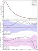 |
Fig. 1 Reconstructed power spectrum of the lensing potential averaged over 300 full-sky lensed simulations. Red dots represent the gradient mode of the deflection (i.e. the lensing potential). Green dots represent the reconstructed curl modes. Middle and bottom panels represent the residuals over 300 lensed simulations of the gradient (middle) and curl (bottom), with the corresponding first-order bias term (black lines). Filled rectangles represent the theoretical dispersion expected for one single reconstruction (Eqs. (27) and (30)). Error bars on the data points are the realization variance on 300 simulations. |
3.1. Filling the point source mask
The first step of the lensing reconstruction pipeline consists in restoring a (fake) signal in the region contaminated by resolved point sources. The aim of this operation is to restore the Gaussian statistics of the temperature map to ensure that the response of the quadratic estimator to this inpainted map will be unchanged compared to the full sky case (i.e. without masking). We will do this by filling the point source holes with a Gaussian realization constrained by the signal around the masked region. This will add some noise in a small area of the sky (≈2%, given the point source mask we use). We will see that this is a small price to be paid for the simplicity to be gained.
We recall here quickly the equation of the Gaussian constrained realizations. The
observed temperature map is decomposed in two parts
 (31)where
T1 represents the regions of the sky which are masked and
need to be inpainted and T2 the regions of the sky which are
used to constrain the value in the masked regions. We also write the covariance matrix Σ
of the temperature field as
(31)where
T1 represents the regions of the sky which are masked and
need to be inpainted and T2 the regions of the sky which are
used to constrain the value in the masked regions. We also write the covariance matrix Σ
of the temperature field as  (32)The joint probability of
(T1,T2) is
given by
(32)The joint probability of
(T1,T2) is
given by ![Mathematical equation: \begin{equation} \mathcal{P}(T_1, T_2)\propto \frac{1}{\sqrt{\rm det( \Sigma)}} \exp\left[{-\frac{1}{2}\left( \begin{array}{c} T_1\\T_2 \end{array} \right)^{\dag} \Sigma^{-1} \left( \begin{array}{c} T_1\\T_2 \end{array} \right ) }\right]. \end{equation}](/articles/aa/full_html/2013/07/aa21048-13/aa21048-13-eq78.png) (33)The probability of
T1 knowing the constraint T2, is
a Gaussian centered on
(33)The probability of
T1 knowing the constraint T2, is
a Gaussian centered on 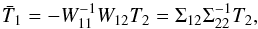 (34)and with a variance
 (35)Given this formalism,
the generation of a local Gaussian constrained realization is straightforward (Hoffman & Ribak 1991). We start by generating a
random realization of the temperature
(35)Given this formalism,
the generation of a local Gaussian constrained realization is straightforward (Hoffman & Ribak 1991). We start by generating a
random realization of the temperature  with a power spectrum
  . As the
variance of the masked regions given the constraints does not depend on the values of the
field, both T1 and
. As the
variance of the masked regions given the constraints does not depend on the values of the
field, both T1 and  have the same variance. We just need to shift the mean of the inpainted region to recover
the expected mean in the masked region. Specifically, we fill the masked regions with the
values
have the same variance. We just need to shift the mean of the inpainted region to recover
the expected mean in the masked region. Specifically, we fill the masked regions with the
values  (36)The computation of this
quantity requires the inversion of Σ22. This operation can be prohibitively
expensive if we use the full CMB as a constraint. However, given the statistical
properties of the CMB temperature anisotropies, the data far away from a given hole will
have a small constraint. This is shown in Fig. 3
where we represent in real space the CMB correlation function as well as the filter we are
constructing above. As we can see the filter is quickly decreasing. This means that we can
reduce the size of the matrix Σ22 by only computing it for the unmasked pixels
in a narrow region around each hole and obtain a good approximation of the result.
(36)The computation of this
quantity requires the inversion of Σ22. This operation can be prohibitively
expensive if we use the full CMB as a constraint. However, given the statistical
properties of the CMB temperature anisotropies, the data far away from a given hole will
have a small constraint. This is shown in Fig. 3
where we represent in real space the CMB correlation function as well as the filter we are
constructing above. As we can see the filter is quickly decreasing. This means that we can
reduce the size of the matrix Σ22 by only computing it for the unmasked pixels
in a narrow region around each hole and obtain a good approximation of the result.
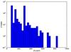 |
Fig. 2 Histogram of the sizes of the holes in our point source mask. |
We perform tests on the constrained Gaussian realizations using three different choices for the size of the constraint region around the holes, with a 10, 15 or 20 pixel borders respectively (corresponding to 34.4, 51.5 and 68.7 arcmin with our HEALPix map resolution). The results of these tests are shown in Fig. 4, which presents the ratio between the mean power spectrum of 100 maps whose point source mask has been filled using the procedure described above and the power spectrum used to perform the random realizations. The different results (depending of the size of the border region used to build the constraint) are to be compared with the green line showing the ratio of the mean power spectrum of the unmasked maps to the input power spectrum. This green line, as expected, nicely varies in the region defined by the black lines, which represent the expected variance for 100 realizations in the (slightly wrong at low ℓ) gaussian approximation for the Cℓ. We clearly see that using only 10 bordering pixels results in an excess of scatter which is probably correlated given its apparent oscillatory behavior. However using 15 or 20 neighboring pixels seems to be acceptable and at the level of precision of our simulation, the power spectrum is nicely recovered without any significant bias.
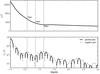 |
Fig. 3 Top panel: CMB correlation as a function of the angular
separation. Bottom: filter corresponding to
|

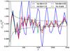 |
Fig. 4 Ratio of the mean of the N = 100 power spectra of the inpainted maps to the fiducial power spectrum for three values of the width of the region used for constraining the Gaussian realization; 10 (blue), 15 (red), and 20 (magenta) pixels. The green line represents the case where no mask is applied. Black lines are the cosmic variance expected given the number of simulations and binning. |
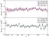 |
Fig. 5 Reconstructed gradient (top) and curl (bottom) modes of the deflection angle on 100 unlensed maps. Point sources are inpainted using 15 (red) to 20 (magenta) bordering pixels to constrain the Gaussian realizations. The unmasked case (green) is shown for comparison. |
3.2. Point sources and lensing reconstruction
We now wish to demonstrate that our treatment of the point source mask is harmless for lensing, i.e. that 1) it does not create any spurious lensing signal; and 2) it enables an excellent reconstruction of the power spectrum of the lensing potential. We first test the case of unlensed maps. In this case, the terms involving the lensing power spectrum disappear and according to Eqs. (26) and (28), the estimated spectrum should be equal to zero. Here again using around 15 to 20 bordering pixels is required in order to get an unbiased reconstruction. Figure 5 shows the mean over 100 lensing reconstructions on unlensed maps. Both the cases with 15 and 20 bordering pixels prove to be in very good agreement with the unmasked case, for both the gradient and curl modes. We thus confirm that the point source inpainting does not create any artificial signal that could be seen as related to lensing via the lensing estimator.
We now turn our analysis on lensed maps. In this case, we need to modify the estimator of
the lensing power spectrum to correct for the fact that the regions that are inpainted are
filled with a perfectly Gaussian realizations and should therefore not contain any lensing
signal. The outputs of the lensing estimator must therefore by rescaled by a factor that
corresponds to the fraction of the signal that is masked. This factor should in principle
be scale dependent as the large scale of the lensing potential are hardly affected by
masking sub-degree scale pixels. However we found that using a scale-independent
renormalization gives an excellent reconstruction of the lensing power spectrum. The
modified estimator reads  (37)where
fPS corresponds to the fraction of the sky which is unmasked
by point sources. With our fiducial point source mask,
fPS = 0.98. Despite theoretical arguments that would naively
lead us to include a
(37)where
fPS corresponds to the fraction of the sky which is unmasked
by point sources. With our fiducial point source mask,
fPS = 0.98. Despite theoretical arguments that would naively
lead us to include a  factor in the normalization, we found on simulations that a
 factor was needed to correctly normalize the estimator.
Figure 6 represents the residuals of the
reconstruction, i.e.  averaged over 300 simulations. We also show the residuals of the curl estimator. We
compare those results to the full-sky case, with no inpainting. As can be seen, there is
no significant difference between the two cases, which validates the use of our inpainting
algorithm for lensing reconstruction.
averaged over 300 simulations. We also show the residuals of the curl estimator. We
compare those results to the full-sky case, with no inpainting. As can be seen, there is
no significant difference between the two cases, which validates the use of our inpainting
algorithm for lensing reconstruction.
We therefore have a tool that can be efficiently used to inpaint the point sources and that can recover both the 2-point and 4-point statistics of a Gaussian field without introducing any spurious signal or bias.
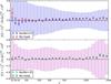 |
Fig. 6 Residuals of the reconstructed power spectrum of the lensing potential averaged over 300 full-sky lensed simulations in presence of the point sources mask. Top panel presents the gradient mode of the deflection (i.e. the lensing potential). Bottom panel presents the reconstructed curl modes. In both cases, we compare with the full-sky case (red for the gradient modes and green for the curl modes). Filled rectangles represent the theoretical dispersion expected for a single reconstruction. |
4. Treatment of the Galactic mask
The second problem frequently encountered in full-sky lens reconstruction is the presence of large-scale foregrounds, primarily along the Galactic plane, which can strongly contaminates the lensing signal. As mentioned in the introduction, several possibilities exist to deal with this complication. We choose a new approach which consists in masking the contaminated regions of the Galactic plane and then directly applying the lensing estimator on those masks maps. We first begin by presenting some analytical computations on the effect of the mask on the reconstructed lensing potential, and we show how these effects can be efficiently alleviated to provide a robust and rapid way of reconstructing the lensing potential.
4.1. Analytical computation of the mask
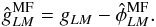
In presence of a mask, the expectation of the lensing estimator becomes
 (38)where
 is a
coupling matrix which replaces the scalar normalization
is a
coupling matrix which replaces the scalar normalization
 , and
, and
 is a lensing independent quantity which we will loosely refer to as the “mask mean field”.
The variance of the estimator applied to a masked temperature map becomes an intricate
expression  (39)where
 denotes the
power spectrum of the mask mean-field.
denotes the
power spectrum of the mask mean-field.  and
and  are
terms similar to the full-sky equivalent
are
terms similar to the full-sky equivalent  and
and  but
also depend on the structure of the mask. All of the terms in the two previous equations
involve high order integrals of functions which can be written as intricate summations of
Wigner 3-j symbols. They are directly related to the structure of the mask and depend on
its harmonic coefficients wℓm. Those
functions and integrals can be written down analytically, but do not lead to a form which
can be efficiently evaluated numerically. However, we find that under certain
circumstances, notably depending on the mask (and we will provide precise examples in
Sect. 4.2), those coupling matrices are essentially
diagonal, in the sense that their effect on power spectra is just to apply a constant
normalization factor. This normalization factor is related to the fraction of the sky
which is unmasked (Hivon et al. 2002). More
precisely, we have
but
also depend on the structure of the mask. All of the terms in the two previous equations
involve high order integrals of functions which can be written as intricate summations of
Wigner 3-j symbols. They are directly related to the structure of the mask and depend on
its harmonic coefficients wℓm. Those
functions and integrals can be written down analytically, but do not lead to a form which
can be efficiently evaluated numerically. However, we find that under certain
circumstances, notably depending on the mask (and we will provide precise examples in
Sect. 4.2), those coupling matrices are essentially
diagonal, in the sense that their effect on power spectra is just to apply a constant
normalization factor. This normalization factor is related to the fraction of the sky
which is unmasked (Hivon et al. 2002). More
precisely, we have  (40)and
 (41)where
 (42)The presence of
the coefficients of the mask to the fourth power is related to the fact that the variance
of the lensing estimator is a resummation of the 4-point correlation function on the CMB.
The variance of the lensing estimator then becomes
(42)The presence of
the coefficients of the mask to the fourth power is related to the fact that the variance
of the lensing estimator is a resummation of the 4-point correlation function on the CMB.
The variance of the lensing estimator then becomes
![Mathematical equation: \begin{equation} \langle g_{LM} g^*_{L^\prime M^\prime}\rangle = \delta_{LL^\prime}\delta_{MM^\prime}f_{\rm{gal},4}\left[ C^{\phi\phi}_{L} + N^{(0,g)}_{L}+ N^{(1,g)}_{L}\right]+ C_L^{\rm{MF}}. \end{equation}](/articles/aa/full_html/2013/07/aa21048-13/aa21048-13-eq109.png) (43)Even though all these
mask kernels cannot be computed, some of them are fairly easy to estimate by a Monte-Carlo
procedure. Applying the estimator on unlensed maps which have the same spectral content as
the lensed map will precisely give the mask mean field
(43)Even though all these
mask kernels cannot be computed, some of them are fairly easy to estimate by a Monte-Carlo
procedure. Applying the estimator on unlensed maps which have the same spectral content as
the lensed map will precisely give the mask mean field
 (44)It is thus
straightforward to construct an unbiased estimator of
by averaging over several outputs of the estimator applied on unlensed masked maps
(44)It is thus
straightforward to construct an unbiased estimator of
by averaging over several outputs of the estimator applied on unlensed masked maps
 (45)
(45) is an unbiased estimate of the mask mean-field and its variance can be approximated by
 (46)We can then define a
mean-field debiased estimator by subtracting the estimated mask mean-field to the lensing
potential reconstructed from the masked temperature field. We therefore define
(46)We can then define a
mean-field debiased estimator by subtracting the estimated mask mean-field to the lensing
potential reconstructed from the masked temperature field. We therefore define
 (47)The
mean of this estimator is
(47)The
mean of this estimator is 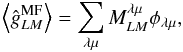 (48)and its variance
becomes
(48)and its variance
becomes ![Mathematical equation: \begin{equation} \langle \hat{g}^{\rm{MF}}_{LM} \hat{g}^{\rm{MF}*}_{L^\prime M^\prime }\rangle \approx \delta_{LL^\prime}\delta_{MM^\prime} f_{\rm{gal},4}\left[ C_L^{\phi\phi} + \left(1+\frac{1}{N_{\rm unl}^{\rm MF}} \right)N^{(0,g)}_{L} + N^{(1,g)}_{L}\right]. \end{equation}](/articles/aa/full_html/2013/07/aa21048-13/aa21048-13-eq116.png) (49)The removal of the mask
mean-field by Monte-Carlo induces a small increase in the variance of the estimator, but
this increase can be made as small as required by averaging over a large number of
unlensed realizations, which is a numerically cheap operation as it does not require the
production of lensed simulations.
(49)The removal of the mask
mean-field by Monte-Carlo induces a small increase in the variance of the estimator, but
this increase can be made as small as required by averaging over a large number of
unlensed realizations, which is a numerically cheap operation as it does not require the
production of lensed simulations.
The estimator of the lensing power spectrum now takes the following form 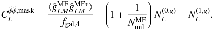 (50)It should also be
noted that for the curl estimator, the situation is somewhat simpler as there is no
mask-mean field (Fig. 9, bottom panel). Therefore
there is no need to subtract a “curl” mask mean field to the curl estimate.
(50)It should also be
noted that for the curl estimator, the situation is somewhat simpler as there is no
mask-mean field (Fig. 9, bottom panel). Therefore
there is no need to subtract a “curl” mask mean field to the curl estimate.
If we now consider the variance of the estimator of the lensing power spectrum, it will
depend on  (51)as it involves
the 8-point correlation function (Kesden et al.
2003; Hanson et al. 2011). We will then
have
(51)as it involves
the 8-point correlation function (Kesden et al.
2003; Hanson et al. 2011). We will then
have ![Mathematical equation: \begin{equation} \sigma^2 \left(C_\ell^{ \tilde \phi \tilde \phi, \rm{mask}}\right) = \frac{f_{\rm{gal},8}}{f^2_{\rm{gal},4}}\frac{2}{2\ell+1} \left[ C_\ell^{\phi\phi, \rm{fid}} + N^{(0,g)}_\ell + N^{(1,g)}_\ell \right]^2. \label{var_mask} \end{equation}](/articles/aa/full_html/2013/07/aa21048-13/aa21048-13-eq119.png) (52)We have set up
the formalism to perform a reconstruction on a masked field. We will now give precise
examples and explain the regime of validity of our approach.
(52)We have set up
the formalism to perform a reconstruction on a masked field. We will now give precise
examples and explain the regime of validity of our approach.
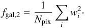
4.2. Apodization
If we apply the quadratic estimator directly to the masked temperature fields, both the mask mean field and the band couplings caused by the presence of the mask will highly bias the reconstruction (Fig. 7), both for the gradient and curl estimator. This behavior is caused by the sharp transition at the boundary of the mask, which creates important power leakage at all scales.
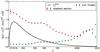 |
Fig. 7 Reconstructed lensing potential (Eq. (50)), averaged over 100 lensed simulations using the binary mask (no apodization). Green dots are the gradient mode which should overlap the black line, and magenta dots the curl modes, which should be compatible with zero. |
In order to reduce the off-diagonal terms in the coupling matrix and the frequency extent of the mask mean field, we simply need to first apodize the mask before masking the temperature field. Apodization smoothes the spectral content of the mask, reduces the mask-mean field amplitude, and removes almost all the off-diagonal terms. This operation has nevertheless a drawback as it decreases the quantity of data used for reconstruction and therefore degrades the statistical significance of the reconstruction. The apodization of the mask is performed by applying a cos-like function to the pixels bordering the mask so that the apodized region goes smoothly from 0 to 1 over the apodization length θapo.
Figure 8 presents the variance of the estimator of
the mask mean field (or equivalently the estimated power spectrum of the mask mean-field)
for both the gradient (top panel) and curl (bottom panel) estimators and for different
values of the apodization length. In all cases, the variance has been rescaled by the
corresponding fgal,4 factor. In this figure,
 . We
here confirm that the mask does not create a mean-field in the curl estimator (bottom
panel). We also see that even a small apodization over 1 degree is enough to remove all
the off-diagonal terms and restore the ability of the quadratic estimator to successfully
reconstruct the lensing power spectrum. In the top panel, we clearly see that the
mean-field decreases when the apodization length is increased. We therefore choose the
higher value, θapo = 10° to perform the
reconstruction. With this value of apodization length, we have
fgal,4 = 0.65.
. We
here confirm that the mask does not create a mean-field in the curl estimator (bottom
panel). We also see that even a small apodization over 1 degree is enough to remove all
the off-diagonal terms and restore the ability of the quadratic estimator to successfully
reconstruct the lensing power spectrum. In the top panel, we clearly see that the
mean-field decreases when the apodization length is increased. We therefore choose the
higher value, θapo = 10° to perform the
reconstruction. With this value of apodization length, we have
fgal,4 = 0.65.
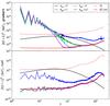 |
Fig. 8 Power spectrum of the mask mean field rescaled by fgal (top, gradient modes; bottom curl modes). The full red line is the Gaussian noise N0,gc divided by the number of unlensed simulation, N = 100. When the binary Galactic mask is applied (blue lines) the reconstruction is strongly biased at high multipoles. Note the absence of a mask mean-field in the curl modes. |
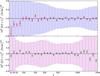 |
Fig. 9 Residuals over 100 lensed simulations of the gradient (top) and curl (bottom) modes of the deflection angle in presence of the Galactic mask, apodized over θapo = 10°. Filled rectangles represent the error bars for one reconstruction (Eq. (52)). |
The final reconstruction is presented in Fig. 9 where we show the mean over 100 residuals of the reconstructed lensing potential power spectrum. In this case, the reconstruction seems less in agreement with the fiducial spectrum at low multipoles, but it should be emphasized that the small bias that can be seen is well with the expected errors bars, whereas the mask-mean field is actually several orders of magnitude higher that the lensing potential at those scales.
4.3. Normalization
The rescaling of the power spectrum of the reconstructed map by
1/fgal,4 can be thought
as a modification of the normalization factor applied to the unnormalized estimator
.
Indeed, rescaling the power spectrum by
1/fgal,4 is equivalent
to applying a normalization factor equal to  . We
can elaborate on this by estimating the normalization factor to apply to the unnormalized
reconstructed potential by computing it by a Monte-Carlo procedure. There are two ways of
doing so, either by correlating the lensing potential reconstructed from a lensed
simulation with the input lensing potential used to generate the lensed temperature map,
or by correlating two lensing reconstructions from two different temperature maps lensed
with the same lensing potential. We thus form the following correlations that define the
mboxMonte-Carlo normalizations
. We
can elaborate on this by estimating the normalization factor to apply to the unnormalized
reconstructed potential by computing it by a Monte-Carlo procedure. There are two ways of
doing so, either by correlating the lensing potential reconstructed from a lensed
simulation with the input lensing potential used to generate the lensed temperature map,
or by correlating two lensing reconstructions from two different temperature maps lensed
with the same lensing potential. We thus form the following correlations that define the
mboxMonte-Carlo normalizations  and
and  :
:
 Here
Here
 and
and  are to be understood as reconstructions from different realizations of temperature maps
lensed with the same lensing potential. As Eq. (53) brings in the two-point correlation function of the masked temperature and
Eq. (54) the four-point correlation
function, relations between ,
and depend on
fgal,2 and
fgal,4, where
are to be understood as reconstructions from different realizations of temperature maps
lensed with the same lensing potential. As Eq. (53) brings in the two-point correlation function of the masked temperature and
Eq. (54) the four-point correlation
function, relations between ,
and depend on
fgal,2 and
fgal,4, where
 (55)More precisely,
we have
(55)More precisely,
we have 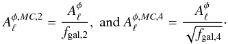 (56)Figure 10 presents the ratio of the normalization computed by
Monte-Carlo to the theoretical normalization. Red dots correspond to
and green dots correspond to
(56)Figure 10 presents the ratio of the normalization computed by
Monte-Carlo to the theoretical normalization. Red dots correspond to
and green dots correspond to  .
The first bin is not in agreement because of the presence of the mask mean field which
yield a non-zero correlation in Eq. (54).
Accordingly, when computing the normalization by correlating the reconstructed lensing
potential to the input potential, the mask mean field disappears from the correlation.
This figure shows a very good agreement between the ratio and the expected constant
values, which validates once again the use of an apodized Galactic mask for CMB lensing
reconstruction. It should be noted that the two normalizations computed here do not have
the same utilization. We have seen previously that
is used to normalize the power spectrum of the reconstructed lensing potential. As
only brings in a single reconstructed potential in its definition, it should be used to
normalize correlations between the reconstructed lensing potential and any other field
that would have a non-zero correlation with the lending potential but not with the
reconstruction noise. A perfect example for such a field would be an external dataset
which also traces large scale structure.
.
The first bin is not in agreement because of the presence of the mask mean field which
yield a non-zero correlation in Eq. (54).
Accordingly, when computing the normalization by correlating the reconstructed lensing
potential to the input potential, the mask mean field disappears from the correlation.
This figure shows a very good agreement between the ratio and the expected constant
values, which validates once again the use of an apodized Galactic mask for CMB lensing
reconstruction. It should be noted that the two normalizations computed here do not have
the same utilization. We have seen previously that
is used to normalize the power spectrum of the reconstructed lensing potential. As
only brings in a single reconstructed potential in its definition, it should be used to
normalize correlations between the reconstructed lensing potential and any other field
that would have a non-zero correlation with the lending potential but not with the
reconstruction noise. A perfect example for such a field would be an external dataset
which also traces large scale structure.
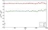 |
Fig. 10 Ratio of the normalization computed by Monte-Carlo to the theoretical normalization in the case of a reconstruction with an apodized Galactic mask. |
5. Point source and galactic mask
All the ingredients are now in place to reconstruct the lensing potential and its power spectrum when both the point sources and Galactic masks are included. The algorithm is fairly simple. We first inpaint the regions masked for point sources using the algorithm described in Sect. 3.1. We then apply the apodized Galactic mask on this inpainted map. We choose to use the largest apodization length we considered previously, θapo = 10°. We then generate a set of unlensed simulations under the lensed temperature power spectrum on which we run the quadratic estimator to estimate the mask mean-field.
Renormalization of the reconstructed lensing potential power spectrum requires some care as
some of the masked regions in the Galactic plane do not have any signal and must therefore
by rescaled by the Galactic mask renormalization value
fgal,4. However the inpainted regions lack
the lensing signal, but possess the full Gaussian structure, so that the Gaussian noise
coming from those regions is the theoretical  . The
estimator of the lensing potential power spectrum then takes the following form
. The
estimator of the lensing potential power spectrum then takes the following form
![Mathematical equation: \begin{equation} C_L^{\tilde \phi \tilde\phi, \rm{mask+PS}}= \frac{1}{f_{\rm{PS}}^2}\left[\frac{\langle g_{LM}g^*_{L M} \rangle }{f_{\rm{gal},4}}- \left(1+\frac{1}{N_{\rm unl}^{\rm MF}} \right)N_L^{(0.g)}\right] - N_L^{(1,g)}\label{rec_clpp_mask_PS}, \end{equation}](/articles/aa/full_html/2013/07/aa21048-13/aa21048-13-eq139.png) (57)and its variance
becomes
(57)and its variance
becomes ![Mathematical equation: \begin{eqnarray} \sigma^2\left(C_\ell^{ \tilde \phi \tilde \phi, \rm{mask+PS}}\right)&=& \frac{f_{\rm{gal},8}}{f^4_{\rm{PS}}f^2_{\rm{gal},4}}\frac{2}{2\ell+1}\\\nonumber &&\times \left[ C_\ell^{\phi\phi, \rm{fid}} +\left(1+\frac{1}{N_{\rm unl}^{\rm MF}} \right) N^{(0,g)}_\ell + N^{(1,g)}_\ell \right]^2. \label{var_maskps} \end{eqnarray}](/articles/aa/full_html/2013/07/aa21048-13/aa21048-13-eq140.png) (58)The
residuals over 300 lensed simulations of the gradient and curl power spectra reconstruction
are presented in Fig. 11. We note the presence of
biases at low multipoles both for gradient and curl modes and at high multipoles for the
curl modes, but their amplitude is small, about 0.1σ. However, the
residuals show excellent agreement with zero in the multipole range
100 ≤ ℓ ≤ 1000, for both the gradient and the curl modes of the deflection
angle. This multipole range is also where the signal-to-noise ratio is the highest, thus
validating the described pipeline.
(58)The
residuals over 300 lensed simulations of the gradient and curl power spectra reconstruction
are presented in Fig. 11. We note the presence of
biases at low multipoles both for gradient and curl modes and at high multipoles for the
curl modes, but their amplitude is small, about 0.1σ. However, the
residuals show excellent agreement with zero in the multipole range
100 ≤ ℓ ≤ 1000, for both the gradient and the curl modes of the deflection
angle. This multipole range is also where the signal-to-noise ratio is the highest, thus
validating the described pipeline.
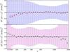 |
Fig. 11 Residuals over 300 simulations of the gradient (top) and curl (bottom) modes of the deflection angle in presence of the point sources mask and of the Galactic mask, apodized over θapo = 10°. Filled rectangles represent the error bars for one reconstruction (Eq. (59)). |
6. Discussion
We have presented a new, simple, and robust pipeline for CMB lensing reconstruction. This pipeline is designed to treat two important issues in a full-sky lensing reconstruction analysis: the presence of point sources that need to be masked and Galactic foregrounds. We treat the first problem by filling in the holes of the temperature map using constrained Gaussian realizations. This operation perfectly restores the Gaussian structure of the original map and inpainted maps can then safely be ingested in the lensing estimator.
The issue of Galactic contamination is treated by simply applying an apodized Galactic mask to the temperature map before the lensing estimation. The presence of the mask creates a bias in the reconstructed potential. However, since this bias is solely related to the mask and does not depend on the actual lensing potential, it can be efficiently estimated from unlensed simulations and then subtracted to the final result. This simple operation is enough to guarantee an unbiased reconstruction of the lensing power spectrum. The contribution of unresolved point sources to the lensed CMB trispectrum is assumed to be small and is therefore ignored.
By using an isotropic filtering during the reconstruction process, this pipeline remains
analytical, in the sense that both the normalization  and the
Gaussian noise
and the
Gaussian noise  keep their
theoretical expression as they are just properly rescaled by scale-independent factor to
account for the missing power due to the presence of masked region.
keep their
theoretical expression as they are just properly rescaled by scale-independent factor to
account for the missing power due to the presence of masked region.
In this article, we have used a simple noise model by considering that the detector noise is white and homogeneous. This will not be the case for a realistic experiment like Planck, where the scanning strategy leads to a non-uniform coverage of the sky. Analytical predictions of the effect of inhomogeneous noise on lensing reconstruction have been investigated in Hanson et al. (2009). The pipeline described in this work can easily be generalized to inhomogeneous noise, by taking into account the noise structure in the unlensed simulations when the mask mean-field is computed. In that case, the estimated mean-field would be the sum of the noise and mask mean-fields. Similarly, any other systematic effects that would create a spurious lensing potential can be treated in a similar way, the difficulty being more in the ability to correctly simulate these effects than in the lensing reconstruction process itself.
Acknowledgments
A.B.L. acknowledges fruitful discussions with E. Hivon. A.B.L. wishes to thank the Jet Propulsion Laboratory (JPL), where part of this work was carried, for kind hospitality. A.B.L. is supported by the Leverhulme Trust and STFC. D.H. acknowledges the support of a CITA National Fellowship. Part of this work has been initiated within the CMB lensing working group of the Planck Collaboration. We also acknowledge the use of the HEALPix package and the cosmological code CAMB.
References
- Basak, S., Prunet, S., & Benabed, K. 2009, A&A, 508, 53 [NASA ADS] [CrossRef] [EDP Sciences] [Google Scholar]
- Benabed, K., & Bernardeau, F. 2000, Phys. Rev. D, 61, 123510 [NASA ADS] [CrossRef] [Google Scholar]
- Benoit-Lévy, A., Smith, K. M., & Hu, W. 2012, Phys. Rev. D, 86, 123008 [NASA ADS] [CrossRef] [Google Scholar]
- Bernardeau, F. 1998, A&A, 338, 767 [NASA ADS] [Google Scholar]
- Blanchard, A., & Schneider, J. 1987, A&A, 184, 1 [NASA ADS] [Google Scholar]
- Cooray, A., Kamionkowski, M., & Caldwell, R. R. 2005, Phys. Rev. D, 71, 123527 [NASA ADS] [CrossRef] [Google Scholar]
- Das, S., Sherwin, B. D., Aguirre, P., et al. 2011, Phys. Rev. Lett., 107, 021301 [NASA ADS] [CrossRef] [Google Scholar]
- Górski, K. M., Hivon, E., Banday, A. J., et al. 2005, ApJ, 622, 759 [NASA ADS] [CrossRef] [Google Scholar]
- Hanson, D., Rocha, G., & Górski, K. 2009, MNRAS, 400, 2169 [NASA ADS] [CrossRef] [Google Scholar]
- Hanson, D., Challinor, A., Efstathiou, G., & Bielewicz, P. 2011, Phys. Rev. D, 83, 043005 [NASA ADS] [CrossRef] [Google Scholar]
- Hirata, C. M., & Seljak, U. C. V. 2003, Phys. Rev. D, 68, 083002 [NASA ADS] [CrossRef] [Google Scholar]
- Hirata, C. M., Ho, S., Padmanabhan, N., Seljak, U. C. V., & Bahcall, N. A. 2008, Phys. Rev. D, 78, 043520 [NASA ADS] [CrossRef] [Google Scholar]
- Hivon, E., Górski, K. M., Netterfield, C. B., et al. 2002, ApJ, 567, 2 [NASA ADS] [CrossRef] [Google Scholar]
- Hoffman, Y., & Ribak, E. 1991, ApJ, 380, L5 [NASA ADS] [CrossRef] [Google Scholar]
- Hu, W. 2000, Phys. Rev. D, 62, 043007 [NASA ADS] [CrossRef] [Google Scholar]
- Hu, W. 2001, Phys. Rev. D, 64, 083005 [NASA ADS] [CrossRef] [Google Scholar]
- Kesden, M., Cooray, A., & Kamionkowski, M. 2003, Phys. Rev. D, 67, 123507 [NASA ADS] [CrossRef] [Google Scholar]
- Knox, L. 1995, Phys. Rev. D, 52, 4307 [NASA ADS] [CrossRef] [Google Scholar]
- Lesgourgues, J., Liguori, M., Matarrese, S., & Riotto, A. 2005, Phys. Rev. D, 71, 103514 [NASA ADS] [CrossRef] [Google Scholar]
- Lesgourgues, J., Perotto, L., Pastor, S., & Piat, M. 2006, Phys. Rev. D, 73, 045021 [NASA ADS] [CrossRef] [Google Scholar]
- Lewis, A., & Challinor, A. 2006, Phys. Rep., 429, 1 [Google Scholar]
- Lewis, A., Challinor, A., & Hanson, D. 2011, JCAP, 3, 18 [NASA ADS] [CrossRef] [Google Scholar]
- Namikawa, T., Yamauchi, D., & Taruya, A. 2012, JCAP, 1, 7 [Google Scholar]
- Okamoto, T., & Hu, W. 2003, Phys. Rev. D, 67, 083002 [NASA ADS] [CrossRef] [Google Scholar]
- Perotto, L., Bobin, J., Plaszczynski, S., Starck, J.-L., & Lavabre, A. 2010, A&A, 519, A4 [NASA ADS] [CrossRef] [EDP Sciences] [Google Scholar]
- Planck Collaboration 2011, A&A, 536, A7 [NASA ADS] [CrossRef] [EDP Sciences] [Google Scholar]
- Planck HFI Core Team 2011, A&A, 536, A6 [NASA ADS] [CrossRef] [EDP Sciences] [Google Scholar]
- Plaszczynski, S., Lavabre, A., Perotto, L., & Starck, J.-L. 2012, A&A, 544, A27 [NASA ADS] [CrossRef] [EDP Sciences] [Google Scholar]
- Smith, K. M., Zahn, O., & Doré, O. 2007, Phys. Rev. D, 76, 043510 [NASA ADS] [CrossRef] [Google Scholar]
- van Engelen, A., Keisler, R., Zahn, O., et al. 2012, ApJ, 756, 142 [NASA ADS] [CrossRef] [Google Scholar]
- Zaldarriaga, M., & Seljak, U. 1999, Phys. Rev. D, 59, 123507 [NASA ADS] [CrossRef] [Google Scholar]
All Figures
|
Fig. 1 Reconstructed power spectrum of the lensing potential averaged over 300 full-sky lensed simulations. Red dots represent the gradient mode of the deflection (i.e. the lensing potential). Green dots represent the reconstructed curl modes. Middle and bottom panels represent the residuals over 300 lensed simulations of the gradient (middle) and curl (bottom), with the corresponding first-order bias term (black lines). Filled rectangles represent the theoretical dispersion expected for one single reconstruction (Eqs. (27) and (30)). Error bars on the data points are the realization variance on 300 simulations. |
| In the text | |
|
Fig. 2 Histogram of the sizes of the holes in our point source mask. |
| In the text | |
|
Fig. 3 Top panel: CMB correlation as a function of the angular
separation. Bottom: filter corresponding to
|
| In the text | |
|
Fig. 4 Ratio of the mean of the N = 100 power spectra of the inpainted maps to the fiducial power spectrum for three values of the width of the region used for constraining the Gaussian realization; 10 (blue), 15 (red), and 20 (magenta) pixels. The green line represents the case where no mask is applied. Black lines are the cosmic variance expected given the number of simulations and binning. |
| In the text | |
|
Fig. 5 Reconstructed gradient (top) and curl (bottom) modes of the deflection angle on 100 unlensed maps. Point sources are inpainted using 15 (red) to 20 (magenta) bordering pixels to constrain the Gaussian realizations. The unmasked case (green) is shown for comparison. |
| In the text | |
|
Fig. 6 Residuals of the reconstructed power spectrum of the lensing potential averaged over 300 full-sky lensed simulations in presence of the point sources mask. Top panel presents the gradient mode of the deflection (i.e. the lensing potential). Bottom panel presents the reconstructed curl modes. In both cases, we compare with the full-sky case (red for the gradient modes and green for the curl modes). Filled rectangles represent the theoretical dispersion expected for a single reconstruction. |
| In the text | |
|
Fig. 7 Reconstructed lensing potential (Eq. (50)), averaged over 100 lensed simulations using the binary mask (no apodization). Green dots are the gradient mode which should overlap the black line, and magenta dots the curl modes, which should be compatible with zero. |
| In the text | |
|
Fig. 8 Power spectrum of the mask mean field rescaled by fgal (top, gradient modes; bottom curl modes). The full red line is the Gaussian noise N0,gc divided by the number of unlensed simulation, N = 100. When the binary Galactic mask is applied (blue lines) the reconstruction is strongly biased at high multipoles. Note the absence of a mask mean-field in the curl modes. |
| In the text | |
|
Fig. 9 Residuals over 100 lensed simulations of the gradient (top) and curl (bottom) modes of the deflection angle in presence of the Galactic mask, apodized over θapo = 10°. Filled rectangles represent the error bars for one reconstruction (Eq. (52)). |
| In the text | |
|
Fig. 10 Ratio of the normalization computed by Monte-Carlo to the theoretical normalization in the case of a reconstruction with an apodized Galactic mask. |
| In the text | |
|
Fig. 11 Residuals over 300 simulations of the gradient (top) and curl (bottom) modes of the deflection angle in presence of the point sources mask and of the Galactic mask, apodized over θapo = 10°. Filled rectangles represent the error bars for one reconstruction (Eq. (59)). |
| In the text | |
Current usage metrics show cumulative count of Article Views (full-text article views including HTML views, PDF and ePub downloads, according to the available data) and Abstracts Views on Vision4Press platform.
Data correspond to usage on the plateform after 2015. The current usage metrics is available 48-96 hours after online publication and is updated daily on week days.
Initial download of the metrics may take a while.