| Issue |
A&A
Volume 555, July 2013
|
|
|---|---|---|
| Article Number | A140 | |
| Number of page(s) | 10 | |
| Section | Interstellar and circumstellar matter | |
| DOI | https://doi.org/10.1051/0004-6361/201219103 | |
| Published online | 15 July 2013 | |
Determination of the far-infrared dust opacity in a prestellar core⋆
1
Department of Physics and AstronomyThe Open University,
Walton Hall Milton Keynes,
MK7 6AA,
UK
e-mail: This email address is being protected from spambots. You need JavaScript enabled to view it.
2
Department of Physics, University of Helsinki,
PO Box 64, 00014
Helsinki,
Finland
3
Finnish Centre for Astronomy with ESO, University of
Turku, Väisäläntie
20, 21500
Piikkiö,
Finland
4
Laboratoire AIM, CEA/DSM-CNRS-Université Paris Diderot,
IRFU/Service d’Astrophysique, CEA Saclay, Orme des Merisiers, 91191
Gif-sur-Yvette,
France
5
Jeremiah Horrocks Institute, University of Central
Lancashire, Preston
PR1 2HE,
UK
6
Institut d’Astrophysique Spatiale, UMR 8617, CNRS/Université
Paris-Sud 11, 91405
Orsay,
France
7
RAL Space, STFC Rutherford Appleton Laboratory,
Chilton Didcot, Oxfordshire
OX11 0QX,
UK
Received:
23
February
2012
Accepted:
11
June
2013
Abstract
Context. Mass estimates of interstellar clouds from far-infrared and submillimetre mappings depend on the assumed dust absorption cross-section for radiation at those wavelengths.
Aims. The aim is to determine the far-IR dust absorption cross-section in a starless, dense core located in Corona Australis. The value is needed for determining of the core mass and other physical properties. It can also have a bearing on the evolutionary stage of the core.
Methods. We correlated near-infrared stellar H − Ks colour excesses of background stars from NTT/SOFI with the far-IR optical depth map, τFIR, derived from Herschel 160, 250, 350, and 500 μm data. The Herschel maps were also used to construct a model for the cloud to examine the effect of temperature gradients on the estimated optical depths and dust absorption cross-sections.
Results. A linear correlation is seen between the colour H − Ks and τFIR up to high extinctions (AV ~ 25). The correlation translates to the average extinction ratio A250 μm/AJ = 0.0014 ± 0.0002, assuming a standard near-infrared extinction law and a dust emissivity index β = 2. Using an empirical NH/AJ ratio we obtain an average absorption cross-section per H nucleus of σH250 μm = (1.8 ± 0.3) × 10-25 cm H-atom, corresponding to a cross-section per unit mass of gas κ250 μmg = 0.08 ± 0.01 cm g. The cloud model, however, suggests that owing to the bias caused by temperature changes along the line-of-sight, these values underestimate the true cross-sections by up to 40% near the centre of the core. Assuming that the model describes the effect of the temperature variation on τFIR correctly, we find that the relationship between H − Ks and τFIR agrees with the recently determined relationship between σH and NH in Orion A.
Conclusions. The derived far-IR cross-section agrees with previous determinations in molecular clouds with moderate column densities, and is not particularly large compared with some other cold cores. We suggest that this is connected to the core not being very dense (the central density is likely to be ~105 cm), and judging from previous molecular line data, it appears to be at an early stage of chemical evolution.
Key words: ISM: clouds / dust, extinction
Based partly on observations collected at the European Southern Observatory, Chile (ESO programmes 075.C-0748 and 077.C-0562).
© ESO, 2013
1. Introduction
Determining the emission properties of interstellar dust is useful not only for providing reliable molecular cloud mass estimates from thermal dust emission maps, but also for testing ideas about dust evolution. In several previous studies the far-infrared to visual or far-IR to near-IR extinction ratio (Aλ/AV or Aλ/AJ), sometimes called the emissivity, has been studied by combining near-infrared photometry and dust continuum maps (Bianchi et al. 2003; Kramer et al. 2003; Shirley et al. 2005; Lehtinen et al. 2007; Shirley et al. 2011). One of the results from these studies is that the dust emissivity changes from region to region, and it shows a tendency to increase with decreasing dust temperature (Arab et al. 2012). This trend agrees well with theoretical predictions, is thought to be caused primarily by dust coagulation in the cold, dense cores of molecular clouds, and is further accentuated by ice formation on the surfaces of dust grains (Ossenkopf & Henning 1994; Stepnik et al. 2003; Paradis et al. 2009; Ormel et al. 2011).
The availability of multi-frequency data from the Planck and Herschel satellites has vastly improved the accuracy of the determination of dust properties and physical conditions in molecular clouds. In particular, the wavelengths accessible to Herschel cover both sides of the emission maximum of cold (T ~ 10 K) interstellar dust. Earlier surveys usually had only two or three frequencies in the submillimetre/far-infrared and often only on one side of the peak.
In this paper we determine the far-infrared dust emissivity and absorption cross-section in a prestellar core using sensitive near-infrared photometry in the H and Ks bands in conjunction with Herschel maps at four wavelengths. In this way we believe we can achieve higher accuracy than previous studies have. Furthermore, the target core provides a useful reference because it has been claimed that it represents a very early stage of chemical evolution where molecular depletion is not significant (Kontinen et al. 2003). The core, which lies in the “tail” of the Corona Australis molecular cloud, can be found in the Planck Early Release Compact Source Catalogue as PLCKECC G359.78-18.341, and has been previously called “CrA C” (Harju et al. 1993) and “SMM 25” (Chini et al. 2003). So far, no indication of star formation taking place in CrA C has been found in the millimetre continuum (Chini et al. 2003), in submillimetre (Herscel), or in the mid- and near-infrared (Peterson et al. 2011).
In Sect. 2 we briefly discuss some aspects of JHK photometry towards highly reddened stars, and in Sect. 3 we describe the near- and far-infrared observations used in the present work. In Sect. 4, the near-IR reddening is correlated with the far-IR optical depth, and the result is used to derive the dust absorption cross-section. Finally, in Sect. 5 we discuss the significance of the obtained results.
2. On JHK photometry at high extinctions
Analysis of JHK near-infrared photometry involves some uncertainties and complications. The JHK system is not uniquely defined because different detectors and filter sets have been used. Additionally the transmissions in the JHK bands depend strongly on the atmospheric transmission (atmospheric HO absorption lines) and thus vary depending on the observing site and is even subject to night-to-night variations. As a consequence one should be careful when comparing photometric data obtained at different epochs and observing sites. This is also true when adapting a JHK reddening slope because these slopes depend on the particular filter-detector combination. The modified Ks is narrower than the K filter and excludes some of the strong atmospheric lines and is thus less influenced by the atmospheric opacity.
The sensitivity of near-infrared observations has increased dramatically during the last decade, and it is now possible to observe routinely highly reddened, faint stars. The reddening affects the observed object spectral energy distribution (SED) and for highly reddened sources the effective wavelength of the filter shifts towards longer wavelengths. This introduces a new effect as the JHK reddening slope changes depending on the reddening. This phenomenon was already noted in the UBV system (see e.g. Golay 1974), and has been later studied e.g. using the Two Micron All Sky Survey (2MASS)2 (Straižys & Lazauskaitė 2008), and the UKIRT Infrared Deep Sky Survey (UKIDSS) data (Stead & Hoare 2009). As noted in Stead & Hoare (2009) one should refer to a reddening track instead of a reddening slope. The importance of the photometric system is highlighted by the fact that in the 2MASS system the reddening track of highly reddened giants curves down in the JHK colour−colour diagram whereas in the MKO system (UKIDSS) the track curves up. In addition to reddening this effect depends on the spectral type of the source. The effect is noticeable for H − K indices larger than ~1.5. In the present work the highest H − Ks indices are nearly 3.
3. Data acquisition
3.1. NTT/SOFI observations
The dense core region of CrA C was imaged in J, H,
and Ks using the Son Of Isaac (SOFI) near-infrared
instrument on the New Technology Telescope (NTT) at the La Silla observatory in May 2005
and July 2006. The SOFI field of view is 4 9 and the pixel
size is 0
9 and the pixel
size is 0 288. The
observing was done using the standard jittering mode in observing blocks of approximately
1 h. Standard stars from the faint near-IR standard list of Persson et al. (1998) were observed frequently during the nights.
Because very few stars were seen in the first J band observing block the
observations were continued only in the H and
Ks bands. The total on source time was 40 min, 104 min and
540 min in the J, H, and Ks
filters, respectively. The average seeing was ~07.
288. The
observing was done using the standard jittering mode in observing blocks of approximately
1 h. Standard stars from the faint near-IR standard list of Persson et al. (1998) were observed frequently during the nights.
Because very few stars were seen in the first J band observing block the
observations were continued only in the H and
Ks bands. The total on source time was 40 min, 104 min and
540 min in the J, H, and Ks
filters, respectively. The average seeing was ~07.
The IRAF3 external package XDIMSUM was used to reduce the imaging data. The images were searched for cosmic rays and sky-subtracted. The two nearest background images in time to each image were used in the sky subtraction. An object mask was constructed for each image. Applying these masks in the sky subtraction produced hole masks for each sky-subtracted image. Special dome flats and illumination correction frames provided by the NTT team were used to flat field and to illumination correct the sky-subtracted SOFI images. Rejection masks combined from a bad pixel mask and individual cosmic ray and hole masks were used when averaging the registered images. The coordinates of the registered images were derived from the 2MASS catalogue (Skrutskie et al. 2006).
The SExtractor software v 2.5.0 (Bertin & Arnouts 1996) package was used to obtain stellar photometry of the reduced SOFI images. Galaxies were excluded using the SExtractor CLASS keyword and by visual inspection of the images.
The zero points of the coadded data were fixed using standard star measurements and
checked using stars in common with the less deep HAWK-I imaging of CrA reported in Sicilia-Aguilar et al. (2011) (see below). The
limiting magnitudes (for a formal error of 0.1 mag) are approximately
21 5,
205, and
208 for
J, H, and Ks,
respectively. After elimination of the nonstellar sources 25, 266, and 369 stars remained
in J, H, and Ks,
respectively. In the subsequent analysis we use the 266 stars detected both in the
H and Ks filters. The locations of these
stars are indicated with blue plus signs in Fig. 4.
As one can see in this Figure, no stars were detected in the very centre of CrA C. All
detections lie at the edges of the core.
5,
205, and
208 for
J, H, and Ks,
respectively. After elimination of the nonstellar sources 25, 266, and 369 stars remained
in J, H, and Ks,
respectively. In the subsequent analysis we use the 266 stars detected both in the
H and Ks filters. The locations of these
stars are indicated with blue plus signs in Fig. 4.
As one can see in this Figure, no stars were detected in the very centre of CrA C. All
detections lie at the edges of the core.
The extracted JHKs magnitudes were converted
into Persson magnitudes, and from these to the 2MASS photometric system as described in
Ascenso et al. (2007). However, these conversion
formulae could not be directly applied to all of the SOFI data because for most stars
J band magnitudes were not available owing to the high extinction.
Using the Eqs. (1)−(6) of Ascenso et al. (2007)
the conversion formula for the (H − Ks) index
from the instrumental magnitudes to the 2MASS system can be written as  (1)where the magnitudes on
the right are SOFI magnitudes. We have attempted to decrease the systematic error arising
from the missing J magnitude by estimating the
(J − Ks) colour using the observed
H − Ks index, the intrinsic
J − K and H − K
colours of giant stars from Bessell & Brett
(1988), and the extinction
ratios A(λ)/A(Ks)
derived by Indebetouw et al. (2005). These give
(1)where the magnitudes on
the right are SOFI magnitudes. We have attempted to decrease the systematic error arising
from the missing J magnitude by estimating the
(J − Ks) colour using the observed
H − Ks index, the intrinsic
J − K and H − K
colours of giant stars from Bessell & Brett
(1988), and the extinction
ratios A(λ)/A(Ks)
derived by Indebetouw et al. (2005). These give
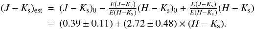 (2)The
ratio of colour excesses
E(J − Ks)/E(H − Ks) = 2.72 ± 0.48
is obtained using the average
A(J)/A(Ks)
and
A(H)/A(Ks)
values listed in Table 1 of Indebetouw et al.
(2005). The corresponding values of
(2)The
ratio of colour excesses
E(J − Ks)/E(H − Ks) = 2.72 ± 0.48
is obtained using the average
A(J)/A(Ks)
and
A(H)/A(Ks)
values listed in Table 1 of Indebetouw et al.
(2005). The corresponding values of  range from 0.27
to 0.50 for giants of the types G0 to M7 using the intrinsic colours given in Bessell & Brett (1988). The possible variation
of the intrinsic colours combined with the uncertainty of the colour excess ratio causes
an additional uncertainty of ~
range from 0.27
to 0.50 for giants of the types G0 to M7 using the intrinsic colours given in Bessell & Brett (1988). The possible variation
of the intrinsic colours combined with the uncertainty of the colour excess ratio causes
an additional uncertainty of ~ to the derived
H − Ks index. This small uncertainty is
added in quadrature to the uncertainties of
H − Ks owing to formal photometric
errors (~
to the derived
H − Ks index. This small uncertainty is
added in quadrature to the uncertainties of
H − Ks owing to formal photometric
errors (~ ) and the uncertainty in
the magnitude zero-point (~
) and the uncertainty in
the magnitude zero-point (~ for
H − Ks).
for
H − Ks).
The conversion to the 2MASS system using Eqs. (1) and (2) reduces the
instrumental H − Ks indices by about 10
percent. The observed H − Ks indices for the
highly reddened stars in our sample range from 15 to
29, and for these
stars the correction lies between  and
and
 . Ignoring the colour-dependent
term in the conversion to the 2MASS system would bias systematically the
H − Ks indices used in the following
analysis.
. Ignoring the colour-dependent
term in the conversion to the 2MASS system would bias systematically the
H − Ks indices used in the following
analysis.
3.2. VLT/HAWK-I observations
The core CrA C was partially covered by two  fields taken with the HAWK-I IR
camera on the VLT as part of the survey of Corona Australis reported in Sicilia-Aguilar et al. (2011) (ESO program 083.C-0079).
A more detailed description of the observations and reduction procedures can be found in
that paper. The photometry zero point of the HAWK-I data was fixed to 2MASS objects
present in the fields. The typical calibration errors range from 1% to 5%, depending on
the weather conditions. Therefore, signal to noise and background remain the main sources
of uncertainty, especially for the fainter objects. The data are complete in the following
dynamical ranges: J = 11−18.5 mag, H = 11−18.5 mag,
K = 10.5−18 mag. The locations of HAWK-I stars with reasonably small
errors (<
fields taken with the HAWK-I IR
camera on the VLT as part of the survey of Corona Australis reported in Sicilia-Aguilar et al. (2011) (ESO program 083.C-0079).
A more detailed description of the observations and reduction procedures can be found in
that paper. The photometry zero point of the HAWK-I data was fixed to 2MASS objects
present in the fields. The typical calibration errors range from 1% to 5%, depending on
the weather conditions. Therefore, signal to noise and background remain the main sources
of uncertainty, especially for the fainter objects. The data are complete in the following
dynamical ranges: J = 11−18.5 mag, H = 11−18.5 mag,
K = 10.5−18 mag. The locations of HAWK-I stars with reasonably small
errors (< in H and
K) lying within a radial distance of
55 from the core
centre are marked with red crosses in Fig. 4. The
total number of these stars is 964.
in H and
K) lying within a radial distance of
55 from the core
centre are marked with red crosses in Fig. 4. The
total number of these stars is 964.
Of the 266 stars in our SOFI sample 109 were detected with HAWK-I. In Fig. 1 we correlate the H − Ks indices of stars common to both surveys. Only a zero-point correction to the 2MASS system has been done to the magnitudes presented in this figure. This is because no colour-dependent correction has been applied to the HAWK-I data (Aurora Sicilia-Aquilar, priv. comm.) as the characteristics of the HAWK-I filters needed for this correction are not available. One can see the uncorrected SOFI colours agree with the HAWK-I data. After the colour correction for SOFI, the slope of the correlation deviates clearly from unity because this correction reduces the H − Ks indices by about 10%. Because our main purpose is to derive the dust opacity towards the core where the colour correction has a noticeable effect, we have decided not to use the HAWK-I data in the subsequent analysis.
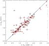 |
Fig. 1 Relationship between the H − Ks colours of the 109 stars detected with both SOFI and HAWK-I, before performing the colour-dependent conversion to the 2MASS system. The photometric errors of the data points are indicated. The solid blue line shows the fit to the data, and the dashed line represents the one-to-one correlation. |
3.3. 2MASS data
Of the stars detected in the 2MASS survey 58 (again, including only those with
ΔK and ΔH ) lie within a distance of
 from the core centre . The
positions of these stars (excluding those coincident with HAWK-I or SOFI stars) are marked
in Fig. 4. Only two of the 2MASS stars coincide with
those in the SOFI sample. The limiting magnitudes of the 2MASS data are
from the core centre . The
positions of these stars (excluding those coincident with HAWK-I or SOFI stars) are marked
in Fig. 4. Only two of the 2MASS stars coincide with
those in the SOFI sample. The limiting magnitudes of the 2MASS data are
 ,
,
 , and
, and
 in J,
H, and K, respectively. Because the 2MASS data clearly
probe the diffuse envelope around the core we will not use them in the derivation of the
submillimetre opacity.
in J,
H, and K, respectively. Because the 2MASS data clearly
probe the diffuse envelope around the core we will not use them in the derivation of the
submillimetre opacity.
3.4. Herschel data
The 15′ × 15′ far-IR and submillimetre maps of CrA C used in this study were extracted from an extensive mapping of the Corona Australis region made as part of the Herschel Gould Belt Survey (André et al. 2010) with the SPIRE (Griffin et al. 2010) and PACS (Poglitsch et al. 2010) instruments onboard Herschel (Pilbratt et al. 2010). The original CrA maps cover a region of about 5° × 2° at the wavelengths 70 and 160 μm (PACS) and 250, 350, and 500 μm (SPIRE). The SPIRE observations were reduced with HIPE 7.0, using modified pipeline scripts, then, the default naive mapping routine was applied to produce the final maps. PACS data was processed within HIPE 8.0 up to level 1 after which we employed Scanamorphos v16 (Roussel 2012) to create the map products. The maps of the whole CrA field will become available on the Herschel Gould Belt Survey Archives4. The beam FWHMs for each wavelength are 36″, 25″, 18″, 12″ × 16″, and 6″ × 12″ for 500, 350, 250, 160, and 70 μm, respectively, the PACS beams being clearly elongated in observations carried out in the parallel mode. The Herschel intensity map at λ = 250 μm, I250 μm, is shown in Fig. 2.
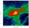 |
Fig. 2 Herschel λ = 250 μm map of CrA C. The contours indicate the intensity I250 μm levels ranging from 50 to 250 MJy/sr. The FWHM of the Herschel beam at this wavelength is 18. |
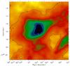 |
Fig. 3 Dust temperature (TD in K) map of CrA C derived from Herschel data. |
Based on comparison with the Planck satellite maps of the region the
following offsets were added to the Herschel maps from 70 to 500
μm, respectively: 2.5, 14.9, 15.6, 8.7, 4.0 MJy/sr. The maps at 160,
250, 350, and 500 μm were convolved to a resolution of 40″ (FWHM), and
the intensity distributions were fitted with a modified blackbody function,
Iν ≈ Bν(Tdust)τν ∝ Bν(Tdust) νβ,
which characterises optically thin thermal dust emission at far-IR and submillimetre
wavelengths. We fixed the emissivity/opacity exponent to β = 2.0. The
resulting Tdust map is shown in Fig. 3. The distribution of the optical depth,
τ(250 μm) = I250 μm/B250 μm(Tdust),
is shown in Fig. 4. On this map we have plotted the
SOFI stars selected for extinction estimates (see below), and the 2MASS and HAWK-I stars
within a radius of of the core centre.
The errors of τ250 μm were estimated from a Monte Carlo method using the 1σ error maps provided for the three SPIRE bands and a 7% uncertainty of the absolute calibration for all four bands according to the information given in SPIRE and PACS manuals (SPIRE Observers’ Manual, Version 2.4; PACS Observer’s Manual, Version 2.4). Different realisations of the τ250 μm map were calculated by combining the four intensity maps with the corresponding error maps, assuming that the error in each pixel is normally distributed. The τ250 μm error in each pixel was obtained from the standard deviation of one thousand realisations.
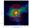 |
Fig. 4 Locations of background stars on the optical depth
τ(250 μm) map from Herschel.
The contour labels give τ(250 μm) values
multiplied by 1000. Different symbols have been used to distinguish between stars
from the three near-IR surveys: 2MASS (green asterisks), HAWK-I (red crosses), and
SOFI (white plus signs). Of the HAWK-I and 2MASS stars only those within a
|
4. Data analysis and results
As we are dealing with a dense core with high near-infrared extinction the number of background stars with accurate J magnitudes is low. To obtain reasonably good statistics, and to extend extinction estimates close to the core centre, we have only used the H and Ks bands where the extinction is less severe than in J. A further motivation for the use of H and Ks is the fact that the intrinsic H − K colours of giants, the class of the background stars most probably observed towards the cloud span a rather narrow range of (H − K)0 = 0.07−0.31 mag (Bessell & Brett 1988). The stellar near-infrared colour excess E(H − K) ≡ (H − K) − (H − K)0 can be used to evaluate the dust column density (Lada et al. 1994).
Because of the reasons discussed in Sects. 2.1−2.3, the HAWK-I and 2MASS stars were used only for checking the zero point of the magnitude scale for the SOFI stars, but not in the estimation of the dust opacity in the CrA C core. For this purpose we used SOFI stars with photometric 1 − σ errors of ΔH < 0.1 mag, ΔK < 0.1 mag. The number of stars fulfilling these criteria is 266. The locations of these stars are indicated with white plus signs in the Herschel far-IR optical depth (τ250 μm) map shown in Fig. 4.
Besides the colour excess E(H − Ks) also the optical depth τ250 μm measures the column density of dust, albeit at very different angular resolution. We have tried to reconcile this difference in the following way: from the Herschel map we have only taken those pixels that contain one or more background stars. The H − Ks value assigned to this pixel is then calculated as the average of the neighbouring stars weighted by a 40″ Gaussian beam to match the resolution of the smoothed dust emission maps. The H − Ks measurements for individual stars taken in the averages were furthermore weighted according to their errors owing to the photometric noise and to the uncertainty of the J − Ks colour needed for the conversion to the 2MASS system as discussed in Sect. 3.1. The errors of the H − Ks values corresponding to pixels in the τ250 μm map were calculated using the standard formula for a weighted average. The resulting correlation plot H − Ks vs. τ(250 μm) is shown in Fig. 5. The typical (mean) error for the colours of the SOFI stars is indicated. The horizontal error bar represents the mean error of the τ250 μm estimates (see Sect. 2.4).
A linear fit to the SOFI data gives the following model (shown in Fig. 5):  The
point where the model intersects the y-axis should represent the average
intrinsic colour (H − Ks)0 of the
background stars. This assumption seems reasonable since the
intersection, 014, corresponds to
the intrinsic H − K colour of a K type giant (Bessell & Brett 1988). Therefore, converting the
far-infrared optical depth to extinction, the fit result can be written as
A(250 μm) = (0.0062 ± 0.0001) E(H − Ks).
Here we have used the relationship
A250 μm = 1.086 τ250 μm.
The
point where the model intersects the y-axis should represent the average
intrinsic colour (H − Ks)0 of the
background stars. This assumption seems reasonable since the
intersection, 014, corresponds to
the intrinsic H − K colour of a K type giant (Bessell & Brett 1988). Therefore, converting the
far-infrared optical depth to extinction, the fit result can be written as
A(250 μm) = (0.0062 ± 0.0001) E(H − Ks).
Here we have used the relationship
A250 μm = 1.086 τ250 μm.
The colour excess can be converted to the near-infrared extinction, e.g.
A(J), using the wavelength dependence of extinction.
According to the extinction ratios,
A(J)/A(Ks) = 2.50 ± 0.15
and
A(H)/A(Ks) = 1.55 ± 0.08,
presented in Table 1 of Indebetouw et al. (2005) the
relationship between A(J) and
E(H − Ks) is
AJ = (4.55 ± 0.72)E(H − Ks).
This relationship is consistent with the extinction law from Cardelli et al. (1989), when the wavelengths of the 2MASS J,
H, and Ks bands are used in their
interpolation formula (2a) and (2b), giving
AJ = 4.44E(H − Ks).
Using the results of Indebetouw et al. (2005) we
obtain the following extinction ratio: 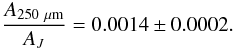 This
extinction ratio is very similar to the value 0.0015 listed in Table 1 of Mathis (1990), and also agrees with the synthetic
extinction law based on the dust model developed by Weingartner & Draine (2001) and Li
& Draine (2001)5. According to the
assumption β = 2.0 used here, the extinction ratio for other wavelengths
longer than 160 μm can be obtained by multiplying the number above by
(250 μm/λ)2.
This
extinction ratio is very similar to the value 0.0015 listed in Table 1 of Mathis (1990), and also agrees with the synthetic
extinction law based on the dust model developed by Weingartner & Draine (2001) and Li
& Draine (2001)5. According to the
assumption β = 2.0 used here, the extinction ratio for other wavelengths
longer than 160 μm can be obtained by multiplying the number above by
(250 μm/λ)2.
To facilitate comparison with some previous results we note that, extrapolating the extinction ratio to the submillimetre regime, our result corresponds to A850 μm/A(Ks) = 3.0 × 10⁻⁴ or A850 μm/AV = 3.9 × 10⁻⁵. In the latter ratio we have assumed that AJ/AV = 0.333 (Cardelli et al. 1989 for RV = 5.5).
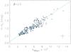 |
Fig. 5 H − Ks colours of the background stars detected with SOFI as a function of far-IR optical depth of the dust emission. The mean error of the data points is indicated with a cross in the bottom right. |
The dust absorption cross-section per H nucleus,  , or per unit mass
of gas,
, or per unit mass
of gas,  , can be estimated
using empirical determinations of the
NH/AJ
or
NH/AV
ratio. As discussed by Martin et al. (2012), the
ratios of near-infrared colour excess, or alternatively near-infrared extinction to
NH are likely to change less than for example the ratio of
AV to NH when
dust grains evolve in dense material. Therefore one could expect that the ratio
NH/AJ
does not change substantially from diffuse to dense clouds.
, can be estimated
using empirical determinations of the
NH/AJ
or
NH/AV
ratio. As discussed by Martin et al. (2012), the
ratios of near-infrared colour excess, or alternatively near-infrared extinction to
NH are likely to change less than for example the ratio of
AV to NH when
dust grains evolve in dense material. Therefore one could expect that the ratio
NH/AJ
does not change substantially from diffuse to dense clouds.
The
NH/E(B − V)
ratio from the Lyα absorption measurement of Bohlin et al. (1978) with the value
RV = 3.1 characteristic of Galactic diffuse
clouds and the corresponding
AJ/AV ratio
(=0.282) give
NH/AJ = 6.6 × 1021 cm-2 mag-1.
Vuong et al. (2003) determined in the dark cloud
ρ Oph
NH/AJ = 5.6−7.2 × 1021 cm-2 mag-1
(depending on the assumed metal abundances) by combining X-ray absorption measurements with
near-infrared photometry. Recently, Martin et al. (2012,
Eq. (9)) compiled a correlation between NH and
E(J − Ks) from several
previous surveys. Their best-fit slope,
NH/E(J − Ks) = (11.5 ± 0.5) × 1021cm-2 mag-1,
together with
AJ/E(J − Ks) = 1.67 ± 0.07
from Indebetouw et al. (2005) imply the ratio
NH/AJ = (6.9 ± 0.4) × 1021 cm-2 mag-1.
Adopting this
NH/AJ ratio
we estimate for σH and κg the
following values:  where
κg is obtained from σH by dividing
it by the average gas particle mass per H nucleus (= 1.4 mH,
assuming 10% He). The range of
NH/AJ
values obtained by Vuong et al. (2003) would imply
where
κg is obtained from σH by dividing
it by the average gas particle mass per H nucleus (= 1.4 mH,
assuming 10% He). The range of
NH/AJ
values obtained by Vuong et al. (2003) would imply
 ,
,
 .
Note that κ is often given per unit mass of dust in which case the number
above should be multiplied by the assumed gas-to-dust mass ratio (usually 100−150).
.
Note that κ is often given per unit mass of dust in which case the number
above should be multiplied by the assumed gas-to-dust mass ratio (usually 100−150).
The values implied by the parameter C250 given in Hildebrand (1983) are
 ,
,
 ,
that is, slightly larger than those obtained above. Again,
,
that is, slightly larger than those obtained above. Again,
 can be converted to
other wavelengths by multiplying by
(250 μm/λ)2. For
160 μm we obtain
can be converted to
other wavelengths by multiplying by
(250 μm/λ)2. For
160 μm we obtain  ,
and extrapolating our value to 850 μm we get
,
and extrapolating our value to 850 μm we get
 .
.
The ratio
A250 μm/AJ
is plotted as a function of Tdust in Fig. 6. One can see that the ratios show a large scatter, but a decreasing
tendency towards higher temperatures can be discerned. A linear fit to the data points gives
the following relationship
A250 μm/AJ = (3.6 ± 0.5) × 10-3 − (1.7 ± 0.4) × 10-4 Tdust,
which suggests that the average ratio increases from 0.0012 to 0.0016 (30%) when
Tdust decreases from 14 K to 12 K. Using the previously quoted
NH/AJ
ratio 6.9 × 1021 cm-2 mag-1 this tendency in the
extinction ratio can be translated to the dust extinction cross-section: the correlation
seems to suggest that increases from
1.5 × 10⁻²⁵ to 2.0 × 10⁻²⁵ when Tdust
decreases from 14 K to 12 K.
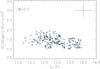 |
Fig. 6 Extinction ratio A250 μm/AJ vs. Tdust. The red line represents a linear fit to the data points using SOFI − Herschel comparison (blue crosses). The mean error of the data points is indicated with a cross in the top right. |
To estimate the effect of the uncertainty related to the adopted emissivity index,
β, and to allow direct comparison with some previous determinations of
the dust opacity (e.g., Martin et al. 2012; Roy et al. 2013; Shirley
et al. 2011), we repeated the analysis described above using fixed emissivity
indices of β = 1.8 and β = 2.2. Lowering
β leads to higher dust colour temperatures, lower optical depths
τ250, and lower values of
. The effect of
increasing β is the opposite. The values of
and
 resulting from a
linear fit to the H − Ks vs.
τ250 μm correlation for
β = 1.8 and β = 2.2 are the following:
resulting from a
linear fit to the H − Ks vs.
τ250 μm correlation for
β = 1.8 and β = 2.2 are the following:
 In
both cases the extrapolated dust absorption cross-section per unit mass of gas at
λ = 850 μm happens to be the same as for
β = 2.0, i.e.,
In
both cases the extrapolated dust absorption cross-section per unit mass of gas at
λ = 850 μm happens to be the same as for
β = 2.0, i.e.,  .
The values at 450 μm change slightly depending on β:
.
The values at 450 μm change slightly depending on β:
 for
β = 1.8−2.2. These results should be compared with predictions from
various models listed in Table 2 of Shirley et al.
(2005).
for
β = 1.8−2.2. These results should be compared with predictions from
various models listed in Table 2 of Shirley et al.
(2005).
The suggested temperature dependence of the
cross-section steepens with the
adopted β. For β = 1.8 the increase in
is about 24% when
Tdust decreases from 14 K to 12 K, whereas for
β = 2.2 the corresponding increase is 37%.
5. Discussion
The extinction ratio
A250 μm/AJ = 0.0014 ± 0.0002,
and the implied values of the dust absorption cross-section,
 ,
and the opacity per unit mass of gas,
,
and the opacity per unit mass of gas,  ,
derived for the cold core CrA C are close to the widely adopted “standard” values from Hildebrand (1983). The derived absorption cross-section
is similar or slightly smaller than the values derived previously for molecular clouds
(e.g., Martin et al. 2012 and references therein).
For example, Terebey et al. (2009) determined the
opacity
κ160 μm = (0.23 ± 0.05) cm2g-1
at 160 μm (assuming β = 2.0) for low extinction regions
(AV up to 4 mag) in the Taurus cloud L1521,
when we get in
CrA C. Adopting the spectral emissivity index β = 1.8 used in several
previous studies, we derive a dust absorption cross-section of
,
derived for the cold core CrA C are close to the widely adopted “standard” values from Hildebrand (1983). The derived absorption cross-section
is similar or slightly smaller than the values derived previously for molecular clouds
(e.g., Martin et al. 2012 and references therein).
For example, Terebey et al. (2009) determined the
opacity
κ160 μm = (0.23 ± 0.05) cm2g-1
at 160 μm (assuming β = 2.0) for low extinction regions
(AV up to 4 mag) in the Taurus cloud L1521,
when we get in
CrA C. Adopting the spectral emissivity index β = 1.8 used in several
previous studies, we derive a dust absorption cross-section of
 .
This value lies close to the low end of the range derived by Martin et al. (2012), using similar methods and the same β,
towards the Vela cloud near the Galactic plane. We note that our
.
This value lies close to the low end of the range derived by Martin et al. (2012), using similar methods and the same β,
towards the Vela cloud near the Galactic plane. We note that our
 has the same meaning
as σe(1200), and that our
is denoted by
rκ0 in Martin et al. Furthermore, we have
adopted the colour excess to column density ratio from Martin et al. (2012). The
τ250/NH ratio
(implying
has the same meaning
as σe(1200), and that our
is denoted by
rκ0 in Martin et al. Furthermore, we have
adopted the colour excess to column density ratio from Martin et al. (2012). The
τ250/NH ratio
(implying  ),
derived by Planck Collaboration (2011) for the
“dense” component (regions detected in CO) of the Taurus Molecular Cloud complex, is larger
than the value obtained here assuming β = 1.8.
),
derived by Planck Collaboration (2011) for the
“dense” component (regions detected in CO) of the Taurus Molecular Cloud complex, is larger
than the value obtained here assuming β = 1.8.
A rough agreement is found with some previous determinatons of the dust opacity in dense
cores. The value of we obtain is similar
to that determined in the Thumbprint Nebula (Lehtinen et al.
1998), and midway the values derived towards two positions in LDN 1688 (Rawlings et al. 2013). Shirley et al. (2011) determined in the protostellar core B335 the opacity ratio
κ850 μm/κK ~ (3.2−4.8) × 10-4,
which agrees with the ratio
κ850 μm/κV ~ 4 × 10⁻⁵
derived by Bianchi et al. (2003) for the starless
globule B68. The opacity ratios determined by Kramer et al.
(2003) in the IC 5146 filament show more variety,
κ850 μm/κV ~ (1.3−5.0) × 10-5,
but there is a clear temperature dependence, and CrA C should be compared with the cool
parts of IC 5146, i.e. the high end of Kramer’s opacity range.
When compared with the frequently used dust model of Ossenkopf & Henning (1994), our average dust opacity
 of gas (~
 of dust) corresponds roughly to the opacity of unprocessed dust grains taken from the MRN
(Mathis et al. 1977) size distribution, but lies
clearly below the predictions for coagulated or/and ice-coated grains of the same model (see
also the comparison between different models in Shirley
et al. 2005).
of dust) corresponds roughly to the opacity of unprocessed dust grains taken from the MRN
(Mathis et al. 1977) size distribution, but lies
clearly below the predictions for coagulated or/and ice-coated grains of the same model (see
also the comparison between different models in Shirley
et al. 2005).
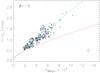 |
Fig. 7 H − K colours of the background stars as a function
τ250 μm from Herschel
assuming a dust emissivity index of β = 1.8. A linear fit to
the data points is shown with a green line. The red curve shows the relationship
implied by the dependence of |
In terms of data and methods used our study is similar to the recent work of Roy et al. (2013) who determined the dust opacities in
the Orion A cloud using Herschel and 2MASS. The study of Roy et al. (2013) benefits from a large number of data
points, majority of them corresponding to moderate extinctions
(AV < 8 mag). The
authors found indications of an increase in the dust opacity towards higher column
densities, with  (see their
Fig. 4). In order to compare this relationship with the situation observed in CrA C, we have
replotted in Fig. 7 the
H − Ks versus
τ250 μm correlation derived using
β = 1.8 as assumed in Roy et al.
(2013). In this figure, we have also plotted the relationship corresponding to the
dependence of
(see their
Fig. 4). In order to compare this relationship with the situation observed in CrA C, we have
replotted in Fig. 7 the
H − Ks versus
τ250 μm correlation derived using
β = 1.8 as assumed in Roy et al.
(2013). In this figure, we have also plotted the relationship corresponding to the
dependence of  on
NH found in Orion A, namely
on
NH found in Orion A, namely
 .
The change of the dust opacity towards higher column densities seems clearly less marked in
CrAC than could have been expected on the basis of the results of Roy et al. (2013) in Orion.
.
The change of the dust opacity towards higher column densities seems clearly less marked in
CrAC than could have been expected on the basis of the results of Roy et al. (2013) in Orion.
The
AFIR/AJ
vs. TD correlation plot suggests, however, a change of
as a function of
temperature (which in turn depends on the column density), and therefore a slight curvature
can be present in the H − Ks vs.
τ250 μm relationship. The slope of the
AFIR/AJ
vs. TD correlation is similar to that derived in L1642 by Lehtinen et al. (2007) for roughly the same temperature
range as observed here, but clearly steeper than the gradient in IC 5146 reported by Kramer et al. (2003) (a factor of three increase in
A850 μm/AV
from Tdust = 20 K to 12 K). The data of Lehtinen et al. suggest
that the gradient in the
AFIR/ANIR ratio
becomes smoother with increasing colour temperature. The implied increase in
with a decreasing
temperature possibly reflects the fact that in starless cores the highest densities are
associated with the lowest dust temperatures. Monte Carlo simulations showed, however, that
if the true relation is flat, noise tends to produce a strong negative correlation between
the observed values of
A250 μm/AJ
and Td. Assuming the 7% relative uncertainty for the surface
brightness measurements, the slope is in the simulations negative and almost three times as
large as the observed one. The 7% error estimate is very conservative for the band-to-band
errors in Herschel data. Nevertheless, we clearly do not have strong
evidence that
A250 μm/AJ
is a decreasing function of temperature in CrA C.
Because of line-of-sight temperature variations, the fitted colour temperature overestimates the mass-averaged dust temperature (e.g., Shetty et al. 2009; Nielbock et al. 2012; Ysard et al. 2012). This leads to an underestimation of the optical depth, τλ, and the dust opacity κλ towards the densest regions (Juvela & Ysard 2012; Malinen et al. 2011).
To estimate the importance of this effect in the present case, we examined a model that
closely resembles the CrA C core. The model is detailed in Appendix A. The modelling result suggests that indeed, the values of
τ250 μm derived from the observations may
underestimate the “true” optical depths of the model by ~30% at the high end of the
H − Ks versus τ correlation.
In Appendix B we examine the change in the
H − Ks versus
τ250 μm correlation assuming that the
relationship between the “observed” and “true” optical depth is the same as in the model. It
turns out that the correlation plot H − Ks
versus the “corrected” τ250 μm agrees quite
well with the relationship implied by the dependence of σH on
NH determined by Roy et al.
(2013), namely that  .
At the high end of the optical depth range examined here, the values of
calculated from this
relationship are ~40% higher than obtained from the linear fit to the unmodified optical
depths derived from observations.
.
At the high end of the optical depth range examined here, the values of
calculated from this
relationship are ~40% higher than obtained from the linear fit to the unmodified optical
depths derived from observations.
To summarise, although we do not see direct evidence for changes of the dust opacity in our
observations, it is likely that the dust temperature in the core decreases inward owing to
the attenuation of the interstellar radiation field, and the optical depths,
τ250 μm, derived from observations
underestimate the true values up to 30% near the core centre. The bias caused by difference
between the colour temperature and the mass-averaged dust temperature was not corrected in
the study of Roy et al. (2013), but probably the
effect there was not as severe as in the present study because their data probe lower column
density regions than that discussed here. Taking the bias into account, and adopting the
emissivity exponent value β = 2.0 we estimate that the dust absorption
cross section per unit mass of gas, , increases from
~0.08 cm2g-1 at the core edges to
~0.11 cm2g-1 close to the centre of the core. We note that the
very nucleus of the core is not sampled in the present data because no stars were detected
in this part.
The dust opacities are not particularly high compared with those found in dense clouds
(e.g., Martin et al. 2012). In the cold cores
examined by Juvela et al. (2011), the highest
estimates were above  cm g but the values obtained for
starless cores in Musca cloud were below
cm g but the values obtained for
starless cores in Musca cloud were below  cm g and thus similar to the
values in CrA C. Owing to its location in the shielded “tail” of the CrA molecular cloud,
near the centre of an extensive HI cloud (Llewellyn et al.
1981; Harju et al. 1993), the CrA C core is
likely to be at an early stage of evolution. Previous molecular line observations support
this idea. Firstly, several common high-density tracers, such as NH, NH and HCO, are weak in
this core, suggesting that the gas has a moderate maximum density
(nH2 ~ 105 cm). This estimate is
consistent with the cloud model constructed in Appendix A where the best fit to the Herschel far-infrared was obtained
with a central density of
nH = 1.5 × 105 cm-3. Secondly, CO
seems to be undepleted and peaks, together with the high-density tracers roughly at the same
place as the thermal dust emission (Kontinen et al.
2003). As grain growth by accretion, and the corresponding depletion of abundant
elements in the gas-phase need time to take effect, the relatively low value of
κ is perhaps connected with the low degree of molecular depletion derived
in CrA C, both being indicators that suggest the relative youth of this core.
cm g and thus similar to the
values in CrA C. Owing to its location in the shielded “tail” of the CrA molecular cloud,
near the centre of an extensive HI cloud (Llewellyn et al.
1981; Harju et al. 1993), the CrA C core is
likely to be at an early stage of evolution. Previous molecular line observations support
this idea. Firstly, several common high-density tracers, such as NH, NH and HCO, are weak in
this core, suggesting that the gas has a moderate maximum density
(nH2 ~ 105 cm). This estimate is
consistent with the cloud model constructed in Appendix A where the best fit to the Herschel far-infrared was obtained
with a central density of
nH = 1.5 × 105 cm-3. Secondly, CO
seems to be undepleted and peaks, together with the high-density tracers roughly at the same
place as the thermal dust emission (Kontinen et al.
2003). As grain growth by accretion, and the corresponding depletion of abundant
elements in the gas-phase need time to take effect, the relatively low value of
κ is perhaps connected with the low degree of molecular depletion derived
in CrA C, both being indicators that suggest the relative youth of this core.
http://irsa.ipac.caltech.edu/Missions/2mass.html
IRAF is distributed by the National Optical Astronomy Observatories, which are operated by the Association of Universities for Research in Astronomy, Inc., under cooperative agreement with the National Science Foundations.
Data available at http://www.astro.princeton.edu/~draine/dust/dustmix.html
Acknowledgments
We thank Aurora Sicilia-Aguilar for providing the HAWK-I photometry of CrA, and Jean-Philippe Bernard for deriving the sky brightness offsets for the Herschel maps using Planck satellite data. Helpful discussions with Kalevi Mattila are thankfully acknowledged. This publication makes use of data products from the Two Micron All Sky Survey, which is a joint project of the University of Massachusetts and the Infrared Processing and Analysis Center/California Institute of Technology, funded by the National Aeronautics and Space Administration and the National Science Foundation. The study has been financially supported by the Academy of Finland through grants 127015, 132291, 140970 and 250741, and by the European Community FP7-ITN Marie-Curie Programme (grant agreement 238258).
References
- André, P., Men'shchikov, A., Bontemps, S., et al. 2010, A&A, 518, L102 [NASA ADS] [CrossRef] [EDP Sciences] [Google Scholar]
- Arab, H., Abergel, A., Habart, E., et al. 2012, A&A, 541, A19 [NASA ADS] [CrossRef] [EDP Sciences] [Google Scholar]
- Ascenso, J., Alves, J., Beletsky, Y., & Lago, M. T. V. T. 2007, A&A, 466, 137 [NASA ADS] [CrossRef] [EDP Sciences] [Google Scholar]
- Bertin, E., & Arnouts, S. 1996, A&AS, 117, 393 [NASA ADS] [CrossRef] [EDP Sciences] [Google Scholar]
- Bessell, M. S., & Brett, J. M. 1988, PASP, 100, 1134 [NASA ADS] [CrossRef] [Google Scholar]
- Bianchi, S., Gonçalves, J., Albrecht, M., et al. 2003, A&A, 399, L43 [NASA ADS] [CrossRef] [EDP Sciences] [Google Scholar]
- Bohlin, R. C., Savage, B. D., & Drake, J. F. 1978, ApJ, 224, 132 [NASA ADS] [CrossRef] [Google Scholar]
- Cardelli, J. A., Clayton, G. C., & Mathis, J. S. 1989, ApJ, 345, 245 [NASA ADS] [CrossRef] [Google Scholar]
- Chini, R., Kämpgen, K., Reipurth, B., et al. 2003, A&A, 409, 235 [NASA ADS] [CrossRef] [EDP Sciences] [Google Scholar]
- Golay, M. 1974, Introduction to astronomical photometry, Astrophys. Space Sci. Lib., 41 [Google Scholar]
- Griffin, M. J., Abergel, A., Abreu, A., et al. 2010, A&A, 518, L3 [Google Scholar]
- Harju, J., Haikala, L. K., Mattila, K., et al. 1993, A&A, 278, 569 [NASA ADS] [Google Scholar]
- Hildebrand, R. H. 1983, QJRAS, 24, 267 [NASA ADS] [Google Scholar]
- Indebetouw, R., Mathis, J. S., Babler, B. L., et al. 2005, ApJ, 619, 931 [NASA ADS] [CrossRef] [Google Scholar]
- Juvela, M., & Ysard, N. 2012, A&A, 539, A71 [NASA ADS] [CrossRef] [EDP Sciences] [Google Scholar]
- Juvela, M., Ristorcelli, I., Pelkonen, V.-M., et al. 2011, A&A, 527, A111 [NASA ADS] [CrossRef] [EDP Sciences] [Google Scholar]
- Kontinen, S., Harju, J., Caselli, P., Heikkilä, A., & Walmsley, M. 2003, in SFChem 2002: Chemistry as a Diagnostic of Star Formation, eds. C. L. Curry, & M. Fich, 331 [Google Scholar]
- Kramer, C., Richer, J., Mookerjea, B., Alves, J., & Lada, C. 2003, A&A, 399, 1073 [NASA ADS] [CrossRef] [EDP Sciences] [Google Scholar]
- Lada, C. J., Lada, E. A., Clemens, D. P., & Bally, J. 1994, ApJ, 429, 694 [NASA ADS] [CrossRef] [Google Scholar]
- Lehtinen, K., Lemke, D., Mattila, K., & Haikala, L. K. 1998, A&A, 333, 702 [NASA ADS] [Google Scholar]
- Lehtinen, K., Juvela, M., Mattila, K., Lemke, D., & Russeil, D. 2007, A&A, 466, 969 [NASA ADS] [CrossRef] [EDP Sciences] [Google Scholar]
- Li, A., & Draine, B. T. 2001, ApJ, 554, 778 [Google Scholar]
- Llewellyn, R., Payne, P., Sakellis, S., & Taylor, K. N. R. 1981, MNRAS, 196, 29P [NASA ADS] [Google Scholar]
- Malinen, J., Juvela, M., Collins, D. C., Lunttila, T., & Padoan, P. 2011, A&A, 530, A101 [NASA ADS] [CrossRef] [EDP Sciences] [Google Scholar]
- Martin, P. G., Roy, A., Bontemps, S., et al. 2012, ApJ, 751, 28 [NASA ADS] [CrossRef] [Google Scholar]
- Mathis, J. S. 1990, ARA&A, 28, 37 [NASA ADS] [CrossRef] [Google Scholar]
- Mathis, J. S., Rumpl, W., & Nordsieck, K. H. 1977, ApJ, 217, 425 [NASA ADS] [CrossRef] [Google Scholar]
- Mathis, J. S., Mezger, P. G., & Panagia, N. 1983, A&A, 128, 212 [NASA ADS] [Google Scholar]
- Nielbock, M., Launhardt, R., Steinacker, J., et al. 2012, A&A, 547, A11 [NASA ADS] [CrossRef] [EDP Sciences] [Google Scholar]
- Ormel, C. W., Min, M., Tielens, A. G. G. M., Dominik, C., & Paszun, D. 2011, A&A, 532, A43 [NASA ADS] [CrossRef] [EDP Sciences] [Google Scholar]
- Ossenkopf, V., & Henning, T. 1994, A&A, 291, 943 [NASA ADS] [Google Scholar]
- Paradis, D., Bernard, J.-P., & Mény, C. 2009, A&A, 506, 745 [NASA ADS] [CrossRef] [EDP Sciences] [Google Scholar]
- Persson, S. E., Murphy, D. C., Krzeminski, W., Roth, M., & Rieke, M. J. 1998, AJ, 116, 2475 [NASA ADS] [CrossRef] [Google Scholar]
- Peterson, D. E., Caratti o Garatti, A., Bourke, T. L., et al. 2011, ApJS, 194, 43 [NASA ADS] [CrossRef] [Google Scholar]
- Pilbratt, G. L., Riedinger, J. R., Passvogel, T., et al. 2010, A&A, 518, L1 [CrossRef] [EDP Sciences] [Google Scholar]
- Planck Collaboration 2011, A&A, 536, A25 [NASA ADS] [CrossRef] [EDP Sciences] [Google Scholar]
- Poglitsch, A., Waelkens, C., Geis, N., et al. 2010, A&A, 518, L2 [NASA ADS] [CrossRef] [EDP Sciences] [Google Scholar]
- Rawlings, M. G., Juvela, M., Lehtinen, K., Mattila, K., & Lemke, D. 2013, MNRAS, 428, 2617 [NASA ADS] [CrossRef] [Google Scholar]
- Roussel, H. 2012 [arXiv:1205.2576] [Google Scholar]
- Roy, A., Martin, P. G., Polychroni, D., et al. 2013, ApJ, 763, 55 [NASA ADS] [CrossRef] [Google Scholar]
- Shetty, R., Kauffmann, J., Schnee, S., Goodman, A. A., & Ercolano, B. 2009, ApJ, 696, 2234 [NASA ADS] [CrossRef] [Google Scholar]
- Shirley, Y. L., Nordhaus, M. K., Grcevich, J. M., et al. 2005, ApJ, 632, 982 [NASA ADS] [CrossRef] [Google Scholar]
- Shirley, Y. L., Huard, T. L., Pontoppidan, K. M., et al. 2011, ApJ, 728, 143 [NASA ADS] [CrossRef] [Google Scholar]
- Sicilia-Aguilar, A., Henning, T., Kainulainen, J., & Roccatagliata, V. 2011, ApJ, 736, 137 [NASA ADS] [CrossRef] [Google Scholar]
- Skrutskie, M. F., Cutri, R. M., Stiening, R., et al. 2006, AJ, 131, 1163 [NASA ADS] [CrossRef] [Google Scholar]
- Stead, J. J., & Hoare, M. G. 2009, MNRAS, 400, 731 [NASA ADS] [CrossRef] [Google Scholar]
- Stepnik, B., Abergel, A., Bernard, J.-P., et al. 2003, A&A, 398, 551 [NASA ADS] [CrossRef] [EDP Sciences] [Google Scholar]
- Straižys, V., & Lazauskaitė, R. 2008, Baltic Astron., 17, 277 [NASA ADS] [Google Scholar]
- Terebey, S., Fich, M., Noriega-Crespo, A., et al. 2009, ApJ, 696, 1918 [NASA ADS] [CrossRef] [Google Scholar]
- Vuong, M. H., Montmerle, T., Grosso, N., et al. 2003, A&A, 408, 581 [NASA ADS] [CrossRef] [EDP Sciences] [Google Scholar]
- Weingartner, J. C., & Draine, B. T. 2001, ApJ, 548, 296 [NASA ADS] [CrossRef] [Google Scholar]
- Ysard, N., Juvela, M., Demyk, K., et al. 2012, A&A, 542, A21 [NASA ADS] [CrossRef] [EDP Sciences] [Google Scholar]
Appendix A: Examining dust temperature in a cloud model of CrA C
The model cloud was discretised to 75 cells, the projected area corresponding to ~7′ × 7′. The temperature distribution in the three-dimensional model was solved with Monte Carlo radiative transfer calculations, assuming the dust properties of Ossenkopf & Henning (1994) (thin ice mantles accreted in 105 years at a density of 10). The predicted surface brightness was compared to the data on CrA C and the column density corresponding to each of the 75 × 75 map pixels was adjusted iteratively until the model exactly reproduced the 250 μm observations. The external radiation field was selected so that also the shape of the model spectra and column density were similar to CrA C. To take into account the shielding by the surrounding cloud, the external field was first attenuated by an amount that corresponds to a dust layer with AV = 1 mag. When the Mathis et al. (1983)
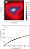 |
Fig. A.1 Results from a radiative transfer model resembling the CrA C core. Frame a) the ratio of the colour temperature (derived from synthetic surface brightness observations) and the mass-averaged real dust temperature. Frame b) the derived values of τ250 μm as the function of the true optical depth in the model. The dotted box corresponds to the range of optical depths in Fig. 7. The dashed green line represents a 1:1 correlation. The red curve represents an exponential function fitted to the data points (see the text). |
field was multiplied with a factor of 5.2, the central column density of the model was ~30% higher than the estimated column density of CrA C and the 160 μm intensity was ~10% above the observed.
The surface brightness maps of the model were analysed in the same way as the real observations, using β = 1.75 applicable for the dust model. As expected, the column density derived from the surface brightness data was below the true values of the model, the error being more than a factor of two at the centre. This is illustrated in Fig. A.1 where the upper frame shows the ratio of the colour temperature and the mass-average dust temperature and the lower frame compares the estimated and the true values of τ250 μm. The bias in the case of CrA C is, of course, not precisely known but can be of similar magnitude, i.e., up to ~30% for the highest optical depths (column densities) considered in the H − K vs. τ250 μm correlation where a similar β has been assumed (Fig. 7). This would decrease the correlation slope and the reported σH and κ250 μm would need to be scaled up. Of course, similar biases may affect most of the values reported in the literature. In what follows we attempt to estimate the effect on σH in more detail.
Appendix B: Dust absorption cross section using the modified optical depths
The relationship between the “observed” and “true” optical depths in the model can be
fitted with the function
τobs = τtrue e−bτtrue,
where b = 28.4. In Fig. B.1, we have
plotted again the observed H − K colours in the
background of CrA C but now against a modified
τ250 μm, assuming the same
conversion between the observed and “true” values as in the model above. In this figure,
we have also plotted the relationship 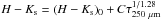 implied by the finding of Roy et al. (2013) in
Orion A that
implied by the finding of Roy et al. (2013) in
Orion A that  . A
reasonable agreement with the data points is achieved by setting the constant
C = 60 instead of 42 which would make the curve bend down too strongly.
This change is equivalent with making the coefficient of proportionality in the
relationship smaller
than in Orion by
. A
reasonable agreement with the data points is achieved by setting the constant
C = 60 instead of 42 which would make the curve bend down too strongly.
This change is equivalent with making the coefficient of proportionality in the
relationship smaller
than in Orion by
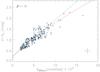 |
Fig. B.1 H − K colours of stars in the background of CrA C
as a function of a modified τ250 μm
where we have attempted to correct for the effect of line-of-sight temperature
variations. It is assumed that the relationship between the observed and “true”
optical depth is similar to the model shown in Fig. A.1. The red curve shows the relationship expected from the result of
Roy et al. (2013) where the
σH increases as
|

a factor of (42/60)1.28 = 0.63. The intersection with the y-axis is the same as in the linear fit, i.e (H − Ks)0 = 0.14. A linear fit to the data, H − Ks = (0.25 ± 0.02) + (167 ± 3) τ250m,true, is also shown in Fig. B.1. The linear fit gives a slightly larger χ2 than the curved relationship. Moreover, the intersection of the line with the y-axis, 0.25, is consistent with an M4 giant (Bessell & Brett 1988) which seems less likely as a typical background star than a K3 giant.
Using the relationships
E(H − Ks) = Cτ1/1.28,
τ = NH σH,
and
NH = E(H − Ks) A(J)/E(H − Ks) NH/A(J)
one obtains the following expression for the dust absorption cross section as a funtion of
the optical depth: 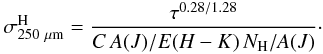 The
dust absorption cross section resulting from this formula is shown in Fig. B.2, for the range of (modified)
τ250 μm estimated for CrA C. Here we
have assumed that C = 60. The model suggests that
increases from the
value 1.2 × 10⁻²⁵ cm2 H-1 to
2.2 × 10⁻²⁵ cm2 H-1 at the largest optical depths,
when the linear fit using the unmodified optical depths gave
The
dust absorption cross section resulting from this formula is shown in Fig. B.2, for the range of (modified)
τ250 μm estimated for CrA C. Here we
have assumed that C = 60. The model suggests that
increases from the
value 1.2 × 10⁻²⁵ cm2 H-1 to
2.2 × 10⁻²⁵ cm2 H-1 at the largest optical depths,
when the linear fit using the unmodified optical depths gave
 .
.
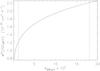 |
Fig. B.2 The dust absorption cross section |
All Figures
|
Fig. 1 Relationship between the H − Ks colours of the 109 stars detected with both SOFI and HAWK-I, before performing the colour-dependent conversion to the 2MASS system. The photometric errors of the data points are indicated. The solid blue line shows the fit to the data, and the dashed line represents the one-to-one correlation. |
| In the text | |
|
Fig. 2 Herschel λ = 250 μm map of CrA C. The contours indicate the intensity I250 μm levels ranging from 50 to 250 MJy/sr. The FWHM of the Herschel beam at this wavelength is 18. |
| In the text | |
|
Fig. 3 Dust temperature (TD in K) map of CrA C derived from Herschel data. |
| In the text | |
|
Fig. 4 Locations of background stars on the optical depth
τ(250 μm) map from Herschel.
The contour labels give τ(250 μm) values
multiplied by 1000. Different symbols have been used to distinguish between stars
from the three near-IR surveys: 2MASS (green asterisks), HAWK-I (red crosses), and
SOFI (white plus signs). Of the HAWK-I and 2MASS stars only those within a
|
| In the text | |
|
Fig. 5 H − Ks colours of the background stars detected with SOFI as a function of far-IR optical depth of the dust emission. The mean error of the data points is indicated with a cross in the bottom right. |
| In the text | |
|
Fig. 6 Extinction ratio A250 μm/AJ vs. Tdust. The red line represents a linear fit to the data points using SOFI − Herschel comparison (blue crosses). The mean error of the data points is indicated with a cross in the top right. |
| In the text | |
|
Fig. 7 H − K colours of the background stars as a function
τ250 μm from Herschel
assuming a dust emissivity index of β = 1.8. A linear fit to
the data points is shown with a green line. The red curve shows the relationship
implied by the dependence of |
| In the text | |
|
Fig. A.1 Results from a radiative transfer model resembling the CrA C core. Frame a) the ratio of the colour temperature (derived from synthetic surface brightness observations) and the mass-averaged real dust temperature. Frame b) the derived values of τ250 μm as the function of the true optical depth in the model. The dotted box corresponds to the range of optical depths in Fig. 7. The dashed green line represents a 1:1 correlation. The red curve represents an exponential function fitted to the data points (see the text). |
| In the text | |
|
Fig. B.1 H − K colours of stars in the background of CrA C
as a function of a modified τ250 μm
where we have attempted to correct for the effect of line-of-sight temperature
variations. It is assumed that the relationship between the observed and “true”
optical depth is similar to the model shown in Fig. A.1. The red curve shows the relationship expected from the result of
Roy et al. (2013) where the
σH increases as
|
| In the text | |
|
Fig. B.2 The dust absorption cross section |
| In the text | |
Current usage metrics show cumulative count of Article Views (full-text article views including HTML views, PDF and ePub downloads, according to the available data) and Abstracts Views on Vision4Press platform.
Data correspond to usage on the plateform after 2015. The current usage metrics is available 48-96 hours after online publication and is updated daily on week days.
Initial download of the metrics may take a while.