| Issue |
A&A
Volume 554, June 2013
|
|
|---|---|---|
| Article Number | A7 | |
| Number of page(s) | 9 | |
| Section | The Sun | |
| DOI | https://doi.org/10.1051/0004-6361/201321428 | |
| Published online | 28 May 2013 | |
Coronal loop physical parameters from the analysis of multiple observed transverse oscillations
1
Instituto de Astrofísica de Canarias,
38205
La Laguna, Tenerife
Spain
e-mail:
This email address is being protected from spambots. You need JavaScript enabled to view it.
2
Departamento de Astrofísica, Universidad de La
Laguna, 38205, La
Laguna, Tenerife,
Spain
Received:
7
March
2013
Accepted:
5
April
2013
Abstract
The analysis of quickly damped transverse oscillations of solar coronal loops using magneto-hydrodynamic seismology allows us to infer physical parameters that are difficult to measure otherwise. Under the assumption that such damped oscillations are due to the resonant conversion of global modes into Alfvén oscillations of the tube surface, we carry out a global seismological analysis of a large set of coronal loops. A Bayesian hierarchical method is used to obtain distributions for coronal loop physical parameters by means of a global analysis of a large number of observations. The resulting distributions summarize global information and constitute data-favoured information that can be used for the inversion of individual events. The results strongly suggest that internal Alfvén travel times along the loop are longer than 100 s and shorter than 540 s with 95% probability. Likewise, the density contrast between the loop interior and the surrounding is larger than 2.3 and below 6.9 with 95% probability.
Key words: magnetohydrodynamics (MHD) / Sun: corona / Sun: oscillations / methods: statistical
© ESO, 2013
1. Introduction
The discovery of quickly damped transverse oscillations of solar coronal loops was first reported by Aschwanden et al. (1999) and Nakariakov et al. (1999) using Transition Region and Coronal Explorer (TRACE) observations. The phenomenon was interpreted in terms of the standing linear magnetohydrodynamic (MHD) kink mode of a magnetic flux tube in its fundamental harmonic. The cause of the quick damping of the oscillations has been attributed to the resonant conversion of global motions into localised Alfvén oscillations at the tube boundary because of the transverse inhomogeneity of the medium (Goossens et al. 2002). The essence of the kink mode has been found to be of mixed nature (Goossens et al. 2009) with a dominant Alfvénic character (Goossens et al. 2012a). Recent reviews on theoretical aspects of MHD kink waves can be found in Ruderman & Erdélyi (2009) and Goossens et al. (2011). Observational properties of transverse coronal loop oscillations are presented and discussed by Schrijver et al. (2002) and Aschwanden et al. (2002).
MHD seismology (Uchida 1970; Roberts et al. 1984) uses inversion techniques to infer difficult-to-measure physical parameters combining theory and observations of MHD waves. Coronal seismology applications using transverse loop oscillation have been successful in determining parameters such as the magnetic field strength (Nakariakov & Ofman 2001), the Alfvén speed (Arregui et al. 2007; Goossens et al. 2008, 2012b), the transversal density structuring (Verwichte et al. 2006), and the coronal density scale height (Andries et al. 2005; Verth et al. 2008; Arregui et al. 2013).
In a previous paper (Arregui & Asensio Ramos 2011), we pursued the Bayesian analysis of individual coronal loops with the aim of inferring their fundamental parameters. In the Bayesian framework the inference is given by the so-called posterior probability distribution, which is a combination of how well the observed data are predicted by the model, the likelihood, and our state of knowledge on the unknowns before considering the data given by the priors. In that analysis, we demonstrated that the inferred values of the Alfvén travel time are robust. Additionally, a Bayesian analysis is able to give some information (or at least put some constraints) on the transverse inhomogeneity. A result of the work was the fact that the density contrast between the coronal loop and the ambient medium is poorly constrained by the observations. The posterior distribution changes when different prior distributions are used for this parameter. However, we demonstrated that the three parameters can be accurately inferred from the period and damping time of the coronal loop oscillations if an independent measurement of the density contrast is available.
These previous studies focused on the inversion of physical parameters using measured wave properties for particular events on a one-by-one basis, thus obtaining estimates for the local properties of the plasma for each particular event. Also, in most of the studies, the wave properties used as input in the inversions consist of quantities that are acquired upon manipulation of parameters obtained at the primary stage of the data analysis. Examples include the use of the period and damping of oscillations obtained after a fitting of the measured time evolution of the displacement in a sequence of imaging observations, as well as the phase speed of propagating waves derived from time-distance diagrams for propagating waves.
This work represents a substantial step forward along two lines. First, we go here to a more fundamental level than Arregui & Asensio Ramos (2011) and use the displacement curves themselves, as measured by Aschwanden et al. (2002), instead of period and damping times. The reason is that the assumption of a Gaussian likelihood function is more appropriate for the displacement curves than for the derived quantities. The noise statistics in the derived quantities is very complicated to obtain, given the non-trivial manipulations that are needed to do this.
Second, a key issue in Bayesian parameter inference is the use of prior information that accounts for our state of knowledge on the unknowns before considering the data. This prior knowledge is usually constructed on the basis of informed guesses about the values and ranges of variation of physical parameters, physical constraints imposed by the model, etc. In this work, we compute these priors using observational information obtained from the global analysis of a number of observed events. This is done by performing a fully consistent analysis of a large number of observations using a hierarchical Bayesian framework. In the same way as directly measured properties of transverse loop oscillations can be summarized by performing histograms, from which quantities such as the mean, median, or standard deviation can be obtained, the Bayesian hierarchical framework enables us to obtain similar information for the physical parameters that cannot be directly measured and thus need to be inferred. As a result, data-favoured distributions for the unknown parameters are obtained. They can then be used to construct priors based on our current observational information of coronal loops.
The layout of the paper is as follows. Section 2 presents our inference approach based on a Bayesian hierarchical model and how this is applied to the observations. The sampling of the posterior and the marginalization is also discussed in this section. Section 3 presents the final results of the paper, and we end with the conclusions in Sect. 4.
2. Hierarchical modeling of coronal loops
If one has direct observational access to a given physical quantity (e.g., brightness or displacement), obtaining an estimation of the probability density for this quantity is easily achieved by just counting events in bins. If observational uncertainties can shift events from one bin to another, it is possible to use Bayesian schemes to take this and other effects into account (e.g., the extreme deconvolution technique of Bovy et al. 2011, and references therein). However, when one is interested in a quantity that cannot be directly observed but has to be inferred from observations, the situation is not so straightforward. This is exactly the problem we have in our case because we do not have direct access to the physical parameters of the oscillating coronal loops. We propose a Bayesian hierarchical scheme to solve this problem. It can be considered as an efficient way to estimate a probability density of an unobserved quantity, which has been obtained from many observations of quantities that are non-linearly related to the one of interest.
In summary, in this work we impose parametric shapes for the priors for all the parameters of interest and learn the value of these parameters from a large set of observed coronal loop oscillations. The ensuing final priors with their shape inferred from the data summarize all the global information we currently have for the physical properties of coronal loop oscillations.
In the following, we first describe the model used to explain the observations and how it depends on the physical parameters of interest. Afterwards, we describe the hierarchical probability model used to explain the complete set of observations and define the hierarchical priors used in this work. We also explain how to efficiently sample the high-dimensional posterior probability distribution function.
2.1. Coronal loops oscillation generative model
Observing oscillations in coronal loops with the aim of carrying out MHD seismology is a
very difficult task. After an arduous process that requires a detailed analysis of the
time evolution of images obtained in coronal lines from space missions, the time variation
of the displacement, d(t), which describes the motion of
the coronal loop apex at different time steps, is obtained (e.g., Aschwanden et al. 2002). To extract information from the time evolution
of the displacement, this quantity is modeled as a combination of a systematic motion of
the entire loop and a real oscillatory component. Therefore, the generative model1 for the observations is then  (1)where
ϵ(t) represents the uncertainty of the amplitude
measurement, while b(t) takes into account the presence
of any remaining uncertainty produced by non-modeled effects like background loops and
wrong estimation of the noise variance. We assume that the uncertainty
ϵ(t) has Gaussian statistics, with zero mean and
time-independent variance
(1)where
ϵ(t) represents the uncertainty of the amplitude
measurement, while b(t) takes into account the presence
of any remaining uncertainty produced by non-modeled effects like background loops and
wrong estimation of the noise variance. We assume that the uncertainty
ϵ(t) has Gaussian statistics, with zero mean and
time-independent variance  . Such a
simplification means that measurements at different times are completely uncorrelated.
Additionally, we use an estimation of σn obtained directly
from the observations. The background component is assumed, for simplicity, to be also
Gaussian with zero mean and time-independent variance
. Such a
simplification means that measurements at different times are completely uncorrelated.
Additionally, we use an estimation of σn obtained directly
from the observations. The background component is assumed, for simplicity, to be also
Gaussian with zero mean and time-independent variance
 .
.
The oscillatory component is modeled in terms of a sinusoidal with an exponential decay
as follows: ![Mathematical equation: \begin{equation} d_\mathrm{osc}(t) = A \sin \left[ \frac{2 \pi}{P} (t-t_0) - \phi_0 \right] \exp \left[- \frac{t-t_0}{\tau_{\rm d}} \right], \end{equation}](/articles/aa/full_html/2013/06/aa21428-13/aa21428-13-eq8.png) (2)where A
is the amplitude of the oscillatory part, P is its period,
t0 is a reference initial time that is fixed from the
observations, φ0 is the initial phase of the oscillation, and
τd is the damping time scale. The detrending of the
oscillatory motion is very difficult to carry out and might depend on an undetermined
(potentially large) number of factors. For this reason, it is customary to use a simple
polynomial function, which absorbs all the unknown effects (Aschwanden et al. 2002):
(2)where A
is the amplitude of the oscillatory part, P is its period,
t0 is a reference initial time that is fixed from the
observations, φ0 is the initial phase of the oscillation, and
τd is the damping time scale. The detrending of the
oscillatory motion is very difficult to carry out and might depend on an undetermined
(potentially large) number of factors. For this reason, it is customary to use a simple
polynomial function, which absorbs all the unknown effects (Aschwanden et al. 2002): 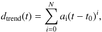 (3)where the
coefficients ai are obtained for each coronal loop and the
order N is adapted to the needed complexity. For simplicity, we fix the
values of the ai coefficients to those obtained by Aschwanden et al. (2002) because no physical information
is extracted from them.
(3)where the
coefficients ai are obtained for each coronal loop and the
order N is adapted to the needed complexity. For simplicity, we fix the
values of the ai coefficients to those obtained by Aschwanden et al. (2002) because no physical information
is extracted from them.
The generative model that we have written does not allow us to extract much physical
information. The period and damping times are purely observational quantities and we need
to relate them to the physical conditions in the loops. To this end, we propose the
resonantly damped MHD kink mode interpretation of quickly damped transverse oscillations
of coronal loops (Ruderman & Roberts 2002;
Goossens et al. 2002) to explain the observed
period P and damping time τd. This
approximation applies to a straight cylindrically symmetric magnetic flux tube with a
uniform magnetic field pointing along the axis of the tube. Under the zero
plasma-β approximation, coronal loops can be considered to be density
enhancements with a constant internal density, ρi, a constant
external density,
ρe < ρi,
and a non-uniform transitional layer of thickness l that connects both
regions. Following Goossens et al. (2008), it is
possible to give the following analytical expression for P and
τd under the thin tube and thin boundary approximations:
 (4)From these
considerations, the parameters in which we are interested are the internal Alfvén travel
time, τA, the density contrast between the tube and the
environment,
ξ = ρi/ρe,
and the transverse inhomogeneity length scale in units of the radius of the loop,
l/R.
(4)From these
considerations, the parameters in which we are interested are the internal Alfvén travel
time, τA, the density contrast between the tube and the
environment,
ξ = ρi/ρe,
and the transverse inhomogeneity length scale in units of the radius of the loop,
l/R.
2.2. Hierarchy
According to the previous model, the oscillatory displacement of the ith coronal loop is determined by the set of parameters θi = { τA,ξ,l/R,A,φ0,σb }, where we use the vector θi to compact the notation. The Bayesian analysis performed by Arregui & Asensio Ramos (2011) demonstrated that the constraining power of the observations is very limited. While τA can be successfully estimated from the observations (although with relatively large and asymmetric error bars), the situation is much worse for the density contrast and the length scale, with the density contrast being the most poorly constrained. Arregui & Asensio Ramos (2011) have shown that the marginal posterior distribution for ξ is very close to the assumed prior distribution, meaning that there is almost no information in the observations to constrain ξ. The reason why, even in the absence of information for the density contrast, the Alfvén travel time can be correctly recovered is related to the specific shapes of the curves in the three-dimensional space (τA,ξ,l/R) pertaining to constant values of P and τd, as explained in Arregui et al. (2007).
We consider
Θ = { θ1,θ2,...,θn }
to be a vector of length 6N that contains all the model parameters for
all the observed N loops. In a standard Bayesian approach, the posterior
distribution (which encodes the updated information about the model parameters) is given
by 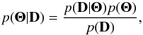 (5)where
D = { D1,D2,...,Dn }
refers to the observed data, the measured time variation of the displacement,
dobs(t), for all the loops. The function
p(D|Θ) is the likelihood, which measures
the probability of getting a set of observed displacements for a given combination of the
parameters. Viewed as a function of the parameters Θ, the likelihood measures
the quality of the parametric model to explain the observations. Finally, the function
p(Θ) is the prior distribution that encodes a priori
information about the model parameters, while p(D) is the
evidence. Given that p(D) does not depend on the model
parameters, it is just a multiplicative constant and can be dropped from the calculations.
(5)where
D = { D1,D2,...,Dn }
refers to the observed data, the measured time variation of the displacement,
dobs(t), for all the loops. The function
p(D|Θ) is the likelihood, which measures
the probability of getting a set of observed displacements for a given combination of the
parameters. Viewed as a function of the parameters Θ, the likelihood measures
the quality of the parametric model to explain the observations. Finally, the function
p(Θ) is the prior distribution that encodes a priori
information about the model parameters, while p(D) is the
evidence. Given that p(D) does not depend on the model
parameters, it is just a multiplicative constant and can be dropped from the calculations.
The quantities with physical interest in our problem are τA,
ξ and l/R. They
are obviously directly unobservable. Consequently, one cannot use the standard histogram
for a set of observed coronal loops with the aim of obtaining their general physical
properties. It is widely known that Bayesian hierarchical models constitute a very
powerful way to overcome this difficulty. The idea behind hierarchical models is extremely
simple. The priors p(Θ) used in Eq. (5) are made dependent on a set of
hyperparameters Ω, which are then included in the inference scheme. Formally,
the posterior is given by 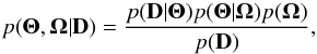 (6)where we have
used the general fact that
p(Θ,Ω) = p(Θ|Ω)p(Ω).
We note that we have dropped the dependence of the likelihood on Ω, given
that Ω are just hyperparameters or, in other words, parameters of the priors.
(6)where we have
used the general fact that
p(Θ,Ω) = p(Θ|Ω)p(Ω).
We note that we have dropped the dependence of the likelihood on Ω, given
that Ω are just hyperparameters or, in other words, parameters of the priors.
If we make the assumption that there is not any correlation between any two coronal loops
from the set of N observations, we can largely simplify Eq. (6). In such a case, the likelihood and the
priors can be factorized, so that the posterior distribution is simplified to read as
 (7)where we have made use of
standard probability calculus.
(7)where we have made use of
standard probability calculus.
Since the global properties of the physical properties are governed by the priors, our
aim is to compute the statistical properties of their parameters, Ω.
Consequently, and although it might seem counterintuitive, all the individual physical
parameters Θ are nuisance parameters for us and have to be integrated out
from the posterior (e.g., Gregory 2005):
 (8)where we have made used
of the fact that the parameters of one loop do not affect those of another loop. This
integration operation propagates information from all individual loops simultaneously to
the hyperparameters.
(8)where we have made used
of the fact that the parameters of one loop do not affect those of another loop. This
integration operation propagates information from all individual loops simultaneously to
the hyperparameters.
2.3. Likelihood
According to the characteristics of the noise and background components of the generative
model displayed in Eq. (1), the likelihood
function is a Gaussian. Given that both ϵ(t) and
b(t) follow the same Gaussian statistics with zero
mean, although with different (time-independent) variances, the total likelihood for an
individual coronal loop is given by
![Mathematical equation: \begin{equation} p(D_{\rm i}|\thetabold_{\rm i}) = \mathcal{C} \exp \left[ -\sum_{j=1}^{m_{\rm i}} \frac{\left(d(t_j)-t_\mathrm{trend}(t_j)-d_\mathrm{osc}(t_j) \right)^2}{2(\sigma_{\rm n}^2+\sigma_{\rm b}^2)}\right] \end{equation}](/articles/aa/full_html/2013/06/aa21428-13/aa21428-13-eq44.png) (9)where
mi is the number of time steps measured for the
ith loop and
(9)where
mi is the number of time steps measured for the
ith loop and  (10)It is important to
have a good estimation of σn, the variance of the noise.
According to Aschwanden et al. (2002), the process
of obtaining the time evolution of the displacement for a given coronal loop is quite
complicated. For this reason, we take a conservative approach and use
σn equal to 10% of the maximum absolute displacement in each
coronal loop. Our results demonstrate that this number is indeed a lower limit to the
actual uncertainty.
(10)It is important to
have a good estimation of σn, the variance of the noise.
According to Aschwanden et al. (2002), the process
of obtaining the time evolution of the displacement for a given coronal loop is quite
complicated. For this reason, we take a conservative approach and use
σn equal to 10% of the maximum absolute displacement in each
coronal loop. Our results demonstrate that this number is indeed a lower limit to the
actual uncertainty.
2.4. Priors
In the hierarchical Bayesian scheme, the definition of suitable priors is as important as the definition of the likelihood. As described in the introduction, the idea is that, since the hyperparameters of the priors are learned from all the data simultaneously, the resulting prior distributions will then be adapted to the data. As a consequence, the prior distributions defined hierarchically are generalizations of the standard calculation of a histogram for quantities that cannot be directly observed, like l/R, τA, and ξ.
To this end, it is favorable to use general probability distributions that naturally
fulfill the boundaries for all the parameters. The first step is to consider the range of
variation of the model parameters. After Goossens et al.
(2008), we know that the model parameters have to fulfill
![Mathematical equation: \begin{equation} l/R \in [0,2], \quad \tau_{\rm A} \geq 0, \quad \xi \gtrsim 1, \quad \phi_0 \in [-\pi,\pi], \quad A \geq 0. \end{equation}](/articles/aa/full_html/2013/06/aa21428-13/aa21428-13-eq47.png) (11)Additionally,
τA and ξ have upper boundaries that do not
emerge from the theory but can be estimated based on physical arguments. We use
(11)Additionally,
τA and ξ have upper boundaries that do not
emerge from the theory but can be estimated based on physical arguments. We use
 s
and ξmax = 100, although their precise values are of reduced
impact in the final result, provided that they are large enough.
s
and ξmax = 100, although their precise values are of reduced
impact in the final result, provided that they are large enough.
The graphical model describing the hierarchy that we consider in the analysis of coronal loop oscillations is shown in Fig. 1. The selected priors, which depend on the set of hyperparameters Ω = { α,β,γ,δ,ϵ,η }, are summarized in Table 1. We give more details in the following.
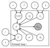 |
Fig. 1 Graphical model representing the hierarchical Bayesian scheme that we used to analyze the set of coronal loop oscillations. Open circles represent random variables (we note that both model parameters and observations are considered as random variables), while the grey circle represents a measured quantity. The frame labeled “Coronal loop i” indicates that the model has to be repeated for all the observations. An arrow between two nodes illustrates dependency. The nodes that are outside the frame are the hyperparameters of the model and are common to all coronal loops. |
Priors used in this work.
2.4.1. Prior for l/R
The theory says that the transverse inhomogeneity length scale has to lie in the
interval [0,2], so it is advisable to use a prior that automatically
fulfills this restriction. We have used a truncated normal distribution that depends on
two parameters, α and β, and is given by
![Mathematical equation: \begin{eqnarray} \mathrm{TN}(l/R;\alpha,\beta) = \left\{ \begin{array}{cc} \left(\!\!\sqrt{2\pi} \beta\right)^{-1} \exp\left[ \!-\!(l/R\!-\!\alpha)^2 \!/\! (2\beta^2) \right] & 0 \leq\! l/R\! \leq 2\nonumber \\[3mm] 0 & \mathrm{otherwise}. \end{array} \right.\\ \end{eqnarray}](/articles/aa/full_html/2013/06/aa21428-13/aa21428-13-eq62.png) (12)Another
option that gives very similar results and also depends on two parameters is the scaled
Beta prior, defined as
(12)Another
option that gives very similar results and also depends on two parameters is the scaled
Beta prior, defined as  (13)where
B(α,β) is the beta function (e.g., Abramowitz & Stegun 1972), which can be
computed in terms of the gamma function as
(13)where
B(α,β) is the beta function (e.g., Abramowitz & Stegun 1972), which can be
computed in terms of the gamma function as
 (14)
(14)
2.4.2. Prior for τA
The Alfvén travel time is defined in the interval [0,∞). A quite
general distribution that is naturally defined in this interval is the inverse gamma
distribution, which depends on two parameters, γ and
δ:  (15)This
distribution has the advantage of describing variables with skewness with only two
parameters. The selection of the inverse gamma distribution is somehow arbitrary, and
other distributions like the gamma distribution can be chosen. We have verified with a
few of them that the results are very robust with respect to the precise selection of
the functional form, provided they have sufficient generality. A few examples of the
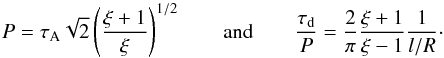
shape of this prior are shown in Fig. 2.
(15)This
distribution has the advantage of describing variables with skewness with only two
parameters. The selection of the inverse gamma distribution is somehow arbitrary, and
other distributions like the gamma distribution can be chosen. We have verified with a
few of them that the results are very robust with respect to the precise selection of
the functional form, provided they have sufficient generality. A few examples of the
shape of this prior are shown in Fig. 2.
2.4.3. Prior for ξ
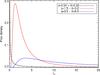 |
Fig. 2 Examples of the IG(γ,δ) distribution, which is a very general distribution for a positive definite quantity. |
The density contrast is a parameter defined in the interval [1,∞),
and scarce information is available as to what the upper limit can be. For this reason,
we choose a shifted inverse gamma distribution, defined as
 (16)
(16)
2.4.4. Prior for σb
The standard deviation of the background contribution, σb,
is inferred from the data. Given that it is a scale parameter, it is customary to use a
Jeffreys’ prior. Because σb is defined in the interval
[0,∞) and the Jeffreys’ prior is neither proper nor well defined at
zero, we propose a modified Jeffreys’ prior (Gregory
2005): ![Mathematical equation: \begin{equation} MJ(\sigma_{\rm b};\sigma_{\rm b}^0,\sigma_{\rm b}^\mathrm{max}) = \left[ \left( \sigma_{\rm b} + \sigma_{\rm b}^0 \right) \ln \left( \frac{\sigma_{\rm b}^0+\sigma_{\rm b}^\mathrm{max}}{\sigma_{\rm b}^0}\right) \right]^{-1}\cdot \end{equation}](/articles/aa/full_html/2013/06/aa21428-13/aa21428-13-eq72.png) (17)This prior behaves as a
Jeffreys’ prior (i.e., as
(17)This prior behaves as a
Jeffreys’ prior (i.e., as  )
for
)
for  and as a
uniform prior for
and as a
uniform prior for  .
Consequently, the transition parameter
.
Consequently, the transition parameter  is a
lower boundary of the Jeffreys’ prior. We chose the small value
is a
lower boundary of the Jeffreys’ prior. We chose the small value
 . We
made sure that this value is sufficiently small so that the posterior for this parameter
peaks at larger values and is therefore not influenced by its actual value. Concerning
. We
made sure that this value is sufficiently small so that the posterior for this parameter
peaks at larger values and is therefore not influenced by its actual value. Concerning
 , it is
made to be very large and its influence on the final results is negligible.
, it is
made to be very large and its influence on the final results is negligible.
2.4.5. Prior for φ0 and A
Without any additional a priori information, we chose a flat prior for the phase of the
oscillation in the interval [−π,π]. This uniform prior equals
(2π)-1 if
− π ≤ φ0 ≤ π and zero
elsewhere. The amplitude of the oscillation is a scale parameter that is defined in the
interval [0,∞). For this reason, we chose a modified Jeffreys’ prior
![Mathematical equation: \begin{equation} MJ(A;A^0,A^\mathrm{max}) = \left[ \left( A + A^0 \right) \ln \left( \frac{A^0+A^\mathrm{max}}{A^0}\right) \right]^{-1}, \end{equation}](/articles/aa/full_html/2013/06/aa21428-13/aa21428-13-eq83.png) (18)with
A0 = 10-3 (much smaller than the actual
amplitude of the oscillation) and a very large Amax.
(18)with
A0 = 10-3 (much smaller than the actual
amplitude of the oscillation) and a very large Amax.
2.4.6. Priors for hyperparameters
The hyperpriors for the hyperparameters α, β, γ, and ϵ are all flat in positive real line. For δ and η, given that they can be considered to be scale parameters, we chose modified Jeffreys’ priors with very small transition parameter. However, the final results are very robust and do not depend on the specific hyperpriors.
2.5. Sampling the posterior
It is clear that the integrals of Eq. (8) cannot be computed analytically. Therefore, it is necessary to rely on numerical techniques. We carry out the integral using a technique based on a Markov chain Monte Carlo (MCMC; Metropolis et al. 1953; Neal 1993). Instead of the general Metropolis-Hastings method, we used a Metropolis-within-Gibbs method (Tierney 1994), which has recently been applied by Sale (2012) for mapping the extinction in the Milky Way using a hierarchical Bayesian model2. The reason for using this scheme is that, in principle, the sampling of the posterior distribution function for every coronal loop is independent of the others, except for the presence of the hyperparameters. Therefore, every step of the posterior sampling for each coronal loop can be done independently. After one iteration of each chain is carried out, the hyperparameters can be updated using a standard Metropolis-Hastings rule. This update is then propagated to every coronal loop. The total length of the converged Markov chains is of the order of a few hundred thousand samples. We verified that the Markov chains are converged using standard criteria. Finally, the initial 30% of the chain is discarded to minimize the sample correlation. As well, we use only one sample out of three to further reduce the correlation.
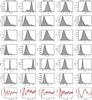 |
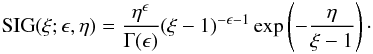
Fig. 3 Posterior distributions for the model parameters of a sample of five coronal loops.
They display the state of knowledge for all physical parameters of all loops when
the observations are taken into account. Shown are the inferred Alfvén travel time
(first row), density contrast (second row),
length scale (third row), standard deviation of the background
(fourth row), derived oscillation period (fifth
row), and damping time (sixth row). The last row shows
the original oscillation corrected for the trend (black curve) and the best fit (red
curve). The black error bars are those associated with
σn, while the red error bars are obtained using
|

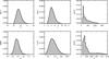 |
Fig. 4 Inferred values for the parameters (hyperparameters) that define the assumed probability distribution functions for l/R, τA and ξ. The hyperparameters α and β define the prior for l/R; γ and δ are used for the prior for τA; ϵ and η define the prior for ξ. |
2.6. Selection of observations
Because of the difficulty of observing oscillations in coronal loops, some of the curves
analyzed by Aschwanden et al. (2002) do not really
display the behavior that we assume in Sect. 2.1.
This poses a problem if the generative model of Eq. (1) does not include the term b(t)
because no combination of the model parameters yields a fit to the observations, whose
residual is Gaussian with zero mean and variance . However,
the inclusion of σb into the inference solves this issue. The
observed loops for which the observation is far from a damped sinusoidal will display a
larger σb.
The total number of coronal loops observed by Aschwanden et al. (2002) is 30. The number of random variables is then 6N + 6 = 186, the model parameters for each loop, including the standard deviation of the background contribution, plus the hyperparameters.
3. Results
3.1. Inference about model parameters
The output of the MCMC code are samples of the model parameters, which are distributed according to the joint posterior p(Θ,Ω|D). To this, we have to add the advantage that the Markov chain for a certain parameter is distributed according to the marginal posterior distribution of this parameter, so the integrals of Eq. (8) are automatically obtained. Figure 3 displays the marginal posteriors for a sample of 5 among the 30 coronal loops that we consider in this work.
The upper row shows the marginal posterior for the Alfvén travel time, which are well constrained in all the cases. The marginal posteriors display a conspicuous peak, although the confidence intervals are clearly asymmetric. This is similar to the findings of Arregui & Asensio Ramos (2011), although in that paper we did not fit the whole time evolution.
The second and third rows show the marginal posteriors for the density contrast and the length scale. It is clear from Eq. (4) that the length scale and the density contrast are intimately related. A fixed value of τd/P can be obtained with an infinite number of combinations of ξ and l/R. Therefore, it is almost impossible to get reliable information for each parameter separately unless strong a priori information is available for any of the two (see Arregui et al. 2007; Arregui & Asensio Ramos 2011). Our results show a very interesting phenomenon that is a direct consequence of the hierarchical scheme. The fact that we assume that the priors for ξ and l/R have to be the same for all the observed coronal loops introduces a large amount of information into the inference. This results in very well-defined posteriors, both for the density contrast and the length scale. Because of the strong constraint imposed by the hierarchical model, the density contrast is roughly the same for all loops and the transverse inhomogeneity length scale is the one to change from loop to loop. We conclude that, under the assumption that the physical properties of all coronal loops are extracted from common probability distribution functions, the damping time scale is fundamentally determined by the transverse inhomogeneity length scale.
The fourth row shows the information inferred for the standard deviation of the background component. Interestingly, σb is always non-negligible, meaning that none of the observed coronal loops displays a pure damped sinusoidal oscillation. Additionally, the distribution is very well defined in all cases, so that it is possible to reliably characterize this background component.
Although τA, ξ, and l/R are the physical parameters behind the model, it is possible to compute the marginal posteriors for derived parameters. Using Eq. (4), we computed the marginal posteriors for the period and the damping time, which are shown in the fifth and sixth rows of Fig. 3. An interesting property of these posteriors is that, although some of the model parameters might not be strongly constrained, P and τd are very well constrained from the observations. The marginal posteriors are very close to Gaussian, which reinforces the assumption used in Arregui & Asensio Ramos (2011) of a Gaussian likelihood with diagonal covariance matrix.
Finally, the lowest row of Fig. 3 displays the measured displacement for each loop and the best fit (roughly equivalent to the least-squares solution, except for the presence of the priors). The black error bars are obtained using the estimated value of σn, while the red error bars are obtained by adding in quadrature σn and σb.
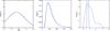 |
Fig. 5 Inferred distributions for the transverse inhomogeneity length scale (left panel), the Alfvén travel time (central panel), and the density contrast between the tube and the environment (right panel). Grey curves represent the marginalized inferred distribution, obtained as the mean of the priors of Sect. 2.4 with parameters distributed according to Fig. 4. Blue lines are the distributions of Sect. 2.4 evaluated at the peak of the distributions of Fig. 4. |
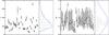 |
Fig. 6 Comparison between the inferred distributions shown in Fig. 5 and a simple histogram carried out with the inferred values of τA and l/R using the formalism of Arregui & Asensio Ramos (2011). |
3.2. Global properties of coronal loops
The hierarchical structure of our model allows us to obtain the general properties of coronal loops. To this end, we show in Fig. 4 the inferred distributions for the hyperparameters that describe the prior distributions described in Sect. 2.4. The first column shows the results for α and β, which are the parameters of the truncated normal distribution for l/R. The results indicate that these hyperparameters have very well-defined values. The median values are αmed ≈ 0.85 and βmed ≈ 0.36. Likewise, the results for the hyperparameters of the prior for τA are also well defined, with γmed ≈ 4.4 and δmed ≈ 870. The situation is less favourable for the hyperparameters of the prior for ξ, probably a consequence of the fact that a single inverse gamma distribution is not able to capture the complexity of the global properties of ξ over the whole sample of coronal loops.
Once the hyperparameters are known, it is possible to use this information to get the
global properties of the physical properties of coronal loops. The first approach is to
follow what is known as the type-II maximum likelihood approximation. In this case, we
simply evaluate the parametric priors defined in Sect. 2.4 at the most probable values of their parameters, which are obtained from the
peaks in Fig. 4. The results are shown as blue lines
in Fig. 5. Another way to fully take into account the
presence of uncertainties in the hyperparameters is to use the
Ns Monte Carlo samples of α,
β, γ, δ, ϵ, and
η from the posterior to evaluate the following marginalized
distributions:  (19)The
previous expressions are the Monte Carlo approximations of the marginalization of the
hyperparameters from the hyperpriors. These distributions are shown as grey lines in Fig.
5.
(19)The
previous expressions are the Monte Carlo approximations of the marginalization of the
hyperparameters from the hyperpriors. These distributions are shown as grey lines in Fig.
5.
The distributions shown in Fig. 5, which constitute the main result of this paper, represent the underlying distribution from which the values of l/R, τA, and ξ have been sampled, under the assumption that this global distribution is shared among all the coronal loops. Consequently, they are generalized histograms of these unobserved quantities, which already take into account any possible degeneracy and uncertainty during the inference process. They represent a data-favored updated prior for the parameters of the model. These priors can be used in the future when making seismological analysis of coronal loops using the resonantly damped MHD kink mode interpretation of quickly damped transverse oscillations.
The left-hand panel of Fig. 5 demonstrates that
roughly all allowed values are possible for the transverse inhomogenity length scale.
However, the slight shift of the distribution shows that there is a small preference for
l/R < 1.
Concerning the Alfvén travel time, it is clear from the central panel of Fig. 5 that the most probable value for
τA is ~160 s, with a median value of ~212 s. The Alfvén
travel time is below ~540 s and above ~100 s with 95% probability. In a unrealistically
oversimplified situation in which the typical length L and density
ρ of the coronal loop is known with precision, the Alfvén travel time
limits that we obtain might be used to put some general constraints on the magnetic field,
given that 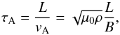 (20)where
vA is the Alfvén velocity and B is the
magnetic field. For instance, if L ~ 100 Mm and
ρ ~ 10-14 g cm-3, we end up with 6 G
≲ B ≲ 35 G. If the density is an order of magnitude larger, the
magnetic field range increases by a factor
(20)where
vA is the Alfvén velocity and B is the
magnetic field. For instance, if L ~ 100 Mm and
ρ ~ 10-14 g cm-3, we end up with 6 G
≲ B ≲ 35 G. If the density is an order of magnitude larger, the
magnetic field range increases by a factor  .
The most probable value of the magnetic field corresponding to the peak of the Alfvén
travel time in Fig. 5 turns out to be
B ~ 16 G. These figures are just estimations based on an unrealistic
situation in which the properties of the coronal loop are known.
.
The most probable value of the magnetic field corresponding to the peak of the Alfvén
travel time in Fig. 5 turns out to be
B ~ 16 G. These figures are just estimations based on an unrealistic
situation in which the properties of the coronal loop are known.
The information gained for the density contrast is also very interesting. We recall that the strong constraint for this parameter is a direct consequence of the hierarchical scheme, which forced the same distribution for all observed coronal loops. According to our results, the density contrast is above 2.3 and below 6.9 with 95% probability, with a median value of 3.8.
Finally, we display in Fig. 6 the comparison between our results and what one would obtain using a simple histogram with the inferred value of the parameters. To this end, we used the inferred values of τA and l/R that were obtained by Arregui & Asensio Ramos (2011), complemented with the results of applying the Bayesian formalism presented by Arregui & Asensio Ramos (2011) to the observations collected in Table 1 of Verwichte et al. (2013). A Jeffreys’ prior in the range [1.2,50] is used for the density contrast, and an uncertainty of 10% is used for the period and damping time if no measurement is available. Although the results are somehow comparable, we note that the error bars are not taken into account in the histogram. This is of special relevance for l/R and less important for τA, where the inferred values are less uncertain.
4. Conclusions
This paper presentes the inference of the global physical properties of coronal loops obtained through MHD seismology. We obtained the inferred distribution of the Alfvén travel time, the size of the transition layer between the surroundings, and the coronal loop density enhancement. These distributions are valid under the assumption that the properties of all coronal loops are just realizations of some underlying distributions. The results demonstrate that sharp transitions between the surrounding and the internal media are slightly favored. Additionally, we have found that Alfvén travel times are in the interval [100,540] s with 95% probability. If the length and density of the coronal loop are known, this poses some constraints on the magnetic field strength in the loop. Likewise, the density contrast between the loop interior and the surrounding is in the interval [2.3,6.9] with 95% probability.
Our contribution is an improvement over our previous approach. First, we made the model closer to the observation by using a generative model to explain the measured displacements. Second, we used a method that obtains global information for model parameters that cannot be directly measured and need to be inferred. Our results allowed us to construct informative priors that can be used for inversions of individual events. The inference then takes into account prior beliefs extracted from data.
Apart from the extraordinary difficulty of extracting the oscillations in coronal loops, the potential to massively apply MHD seismology techniques is now larger than ever thanks
to the continuous observations of the Atmospheric Imaging Assembly (AIA; Lemen et al. 2012) on board the Solar Dynamics Observatory. Their high temporal cadence of 12 s and high spatial resolution of ~0.6 arcsec make them the perfect instrument to follow these oscillatory events and extract reliable physical information from these coronal events.
A generative model defines a parametric description of the signal, taking into account the presence of observational uncertainties and its statistical properties.
IDL and Fortran 2003 codes can be downloaded from https://github.com/aasensio/mcmc
Acknowledgments
We are grateful to Markus J. Aschwanden for kindly providing the measurements of coronal loops oscillations used in this paper. We thank M. J. Martínez González, R. Manso Sainz, M. J. Aschwanden, and R. Oliver for useful suggestions to improve the quality of the manuscript. Financial support by the Spanish Ministry of Economy and Competitiveness through projects AYA2010–18029 (Solar Magnetism and Astrophysical Spectropolarimetry) and AYA2011-22846 is gratefully acknowledged. We also acknowledge financial support through the Ramón y Cajal fellowships and the Consolider-Ingenio 2010 CSD2009-00038 project.
References
- Abramowitz, M., & Stegun, I. A. 1972, Handbook of Mathematical Functions (New York: Dover) [Google Scholar]
- Andries, J., Arregui, I., & Goossens, M. 2005, ApJ, 624, L57 [NASA ADS] [CrossRef] [Google Scholar]
- Arregui, I., & AsensioRamos, A. 2011, ApJ, 740, 44 [NASA ADS] [CrossRef] [Google Scholar]
- Arregui, I., Andries, J., Van Doorsselaere, T., Goossens, M., & Poedts, S. 2007, A&A, 463, 333 [NASA ADS] [CrossRef] [EDP Sciences] [Google Scholar]
- Arregui, I., Asensio Ramos, A., & Díaz, A. J. 2013, ApJ, in press [Google Scholar]
- Aschwanden, M. J., Fletcher, L., Schrijver, C. J., & Alexander, D. 1999, ApJ, 520, 880 [NASA ADS] [CrossRef] [Google Scholar]
- Aschwanden, M. J., de Pontieu, B., Schrijver, C. J., & Title, A. M. 2002, Sol. Phys., 206, 99 [NASA ADS] [CrossRef] [Google Scholar]
- Bovy, J., Hogg, D. W., & Roweis, S. T. 2011, Ann. Appl. Statist., 5, 1657 [Google Scholar]
- Goossens, M., Andries, J., & Aschwanden, M. J. 2002, A&A, 394, L39 [NASA ADS] [CrossRef] [EDP Sciences] [Google Scholar]
- Goossens, M., Arregui, I., Ballester, J. L., & Wang, T. J. 2008, A&A, 484, 851 [NASA ADS] [CrossRef] [EDP Sciences] [Google Scholar]
- Goossens, M., Terradas, J., Andries, J., Arregui, I., & Ballester, J. L. 2009, A&A, 503, 213 [NASA ADS] [CrossRef] [EDP Sciences] [Google Scholar]
- Goossens, M., Erdélyi, R., & Ruderman, M. S. 2011, Space Sci. Rev., 158, 289 [NASA ADS] [CrossRef] [Google Scholar]
- Goossens, M., Andries, J., Soler, R., et al. 2012a, ApJ, 753, 111 [NASA ADS] [CrossRef] [Google Scholar]
- Goossens, M., Soler, R., Arregui, I., & Terradas, J. 2012b, ApJ, 760, 98 [NASA ADS] [CrossRef] [Google Scholar]
- Gregory, P. C. 2005, Bayesian Logical Data Analysis for the Physical Sciences (Cambridge: Cambridge University Press) [Google Scholar]
- Lemen, J. R., Title, A. M., Akin, D. J., et al. 2012, Sol. Phys., 275, 17 [NASA ADS] [CrossRef] [Google Scholar]
- Metropolis, N., Rosenbluth, A. W., Rosenbluth, M. N., Teller, A. H., & Teller, E. 1953, J. Chem. Phys., 21, 1087 [NASA ADS] [CrossRef] [Google Scholar]
- Nakariakov, V. M., & Ofman, L. 2001, A&A, 372, L53 [NASA ADS] [CrossRef] [EDP Sciences] [Google Scholar]
- Nakariakov, V. M., Ofman, L., Deluca, E. E., Roberts, B., & Davila, J. M. 1999, Science, 285, 862 [NASA ADS] [CrossRef] [PubMed] [Google Scholar]
- Neal, R. M. 1993, Probabilistic Inference Using Markov Chain Monte Carlo Methods (Dept. of Statistics, University of Toronto: Technical Report No. 0506) [Google Scholar]
- Roberts, B., Edwin, P. M., & Benz, A. O. 1984, ApJ, 279, 857 [NASA ADS] [CrossRef] [Google Scholar]
- Ruderman, M. S., & Erdélyi, R. 2009, Space Sci. Rev., 149, 199 [NASA ADS] [CrossRef] [Google Scholar]
- Ruderman, M. S., & Roberts, B. 2002, ApJ, 577, 475 [NASA ADS] [CrossRef] [Google Scholar]
- Sale, S. E. 2012, MNRAS, 427, 2119 [NASA ADS] [CrossRef] [Google Scholar]
- Schrijver, C. J., Aschwanden, M. J., & Title, A. M. 2002, Sol. Phys., 206, 69 [NASA ADS] [CrossRef] [Google Scholar]
- Tierney, L. 1994, Ann. Statis., 22, 2701 [Google Scholar]
- Uchida, Y. 1970, PASJ, 22, 341 [NASA ADS] [Google Scholar]
- Verth, G., Erdélyi, R., & Jess, D. B. 2008, ApJ, 687, L45 [NASA ADS] [CrossRef] [Google Scholar]
- Verwichte, E., Foullon, C., & Nakariakov, V. M. 2006, A&A, 452, 615 [NASA ADS] [CrossRef] [EDP Sciences] [Google Scholar]
- Verwichte, E., Van Doorsselaere, T., White, R. S., & Antolin, P. 2013, A&A, 552, A138 [NASA ADS] [CrossRef] [EDP Sciences] [Google Scholar]
All Tables
All Figures
|
Fig. 1 Graphical model representing the hierarchical Bayesian scheme that we used to analyze the set of coronal loop oscillations. Open circles represent random variables (we note that both model parameters and observations are considered as random variables), while the grey circle represents a measured quantity. The frame labeled “Coronal loop i” indicates that the model has to be repeated for all the observations. An arrow between two nodes illustrates dependency. The nodes that are outside the frame are the hyperparameters of the model and are common to all coronal loops. |
| In the text | |
|
Fig. 2 Examples of the IG(γ,δ) distribution, which is a very general distribution for a positive definite quantity. |
| In the text | |
|
Fig. 3 Posterior distributions for the model parameters of a sample of five coronal loops.
They display the state of knowledge for all physical parameters of all loops when
the observations are taken into account. Shown are the inferred Alfvén travel time
(first row), density contrast (second row),
length scale (third row), standard deviation of the background
(fourth row), derived oscillation period (fifth
row), and damping time (sixth row). The last row shows
the original oscillation corrected for the trend (black curve) and the best fit (red
curve). The black error bars are those associated with
σn, while the red error bars are obtained using
|
| In the text | |
|
Fig. 4 Inferred values for the parameters (hyperparameters) that define the assumed probability distribution functions for l/R, τA and ξ. The hyperparameters α and β define the prior for l/R; γ and δ are used for the prior for τA; ϵ and η define the prior for ξ. |
| In the text | |
|
Fig. 5 Inferred distributions for the transverse inhomogeneity length scale (left panel), the Alfvén travel time (central panel), and the density contrast between the tube and the environment (right panel). Grey curves represent the marginalized inferred distribution, obtained as the mean of the priors of Sect. 2.4 with parameters distributed according to Fig. 4. Blue lines are the distributions of Sect. 2.4 evaluated at the peak of the distributions of Fig. 4. |
| In the text | |
|
Fig. 6 Comparison between the inferred distributions shown in Fig. 5 and a simple histogram carried out with the inferred values of τA and l/R using the formalism of Arregui & Asensio Ramos (2011). |
| In the text | |
Current usage metrics show cumulative count of Article Views (full-text article views including HTML views, PDF and ePub downloads, according to the available data) and Abstracts Views on Vision4Press platform.
Data correspond to usage on the plateform after 2015. The current usage metrics is available 48-96 hours after online publication and is updated daily on week days.
Initial download of the metrics may take a while.