| Issue |
A&A
Volume 554, June 2013
|
|
|---|---|---|
| Article Number | A53 | |
| Number of page(s) | 5 | |
| Section | The Sun | |
| DOI | https://doi.org/10.1051/0004-6361/201321075 | |
| Published online | 04 June 2013 | |
Vertical flows and mass flux balance of sunspot umbral dots
1 Max-Planck-Institut für Sonnensystemforschung (MPS), Max-Planck-Str. 2, 37191 Katlenburg-Lindau, Germany
e-mail: This email address is being protected from spambots. You need JavaScript enabled to view it.
; This email address is being protected from spambots. You need JavaScript enabled to view it.
; This email address is being protected from spambots. You need JavaScript enabled to view it.
, This email address is being protected from spambots. You need JavaScript enabled to view it.
2 Technische Universität Braunschweig, Institut für Geophysik und Extraterrestrische Physik, Mendelssohnstr. 3, 38106 Braunschweig, Germany
3 School of Space Research, Kyung Hee University, Yongin, 446-701 Gyeonggi, Republic of Korea
Received: 10 January 2013
Accepted: 30 April 2013
Abstract
A new Stokes inversion technique that greatly reduces the effect of the spatial point spread function of the telescope is used to constrain the physical properties of umbral dots (UDs). The depth-dependent inversion of the Stokes parameters from a sunspot umbra recorded with Hinode SOT/SP revealed significant temperature enhancements and magnetic field weakenings in the core of the UDs in deep photospheric layers. Additionally, we found upflows of around 960 m/s in peripheral UDs (i.e., UDs close to the penumbra) and ≈600 m/s in central UDs. For the first time, we also detected systematic downflows for distances larger than 200 km from the UD center that balance the upflowing mass flux. In the upper photosphere, we found almost no difference between the UDs and their diffuse umbral background.
Key words: Sun: photosphere / sunspots / techniques: polarimetric
© ESO, 2013
1. Introduction
Umbral dots (UDs) are small brightness enhancements in sunspot umbrae or pores and were first detected by Chevalier (1916). The strong vertical magnetic field in umbrae suppresses the energy transport by convection (Biermann 1941), but some form of remaining heat transport is needed to explain the observed umbral brightness (Adjabshirzadeh & Koutchmy 1983). Magnetoconvection in umbral fine structure, such as UDs and light bridges, is thought to be the main contributor to the energy transport in the umbra (Weiss 2002), see reviews by Solanki (2003), Sobotka (2006), and Borrero & Ichimoto (2011).
Progress in the physical understanding of umbral dots was made with numerical simulations of 3D radiative magnetoconvection (Schüssler & Vögler 2006; Bharti et al. 2010). Most of the simulated UDs have a horizontally elongated shape and show a central dark lane in their bolometric intensity images. In the deepest photospheric layers, the inner parts of UDs exhibit magnetic-field weakenings and upflow velocities. The simulated UDs are surrounded by downflows that are often concentrated in narrow downflow channels at the endpoints of the dark lanes (Schüssler & Vögler 2006). Higher up in the photosphere, the UDs in the simulations do not differ significantly from the diffuse background.
Considerable efforts on the observational side were made to test these theoretical predictions. Dark lanes inside UDs were found in the observations of Bharti et al. (2007) with the 50-cm Hinode telescope and by Rimmele (2008), who observed with the 76-cm Dunn Solar Telescope. However, Louis et al. (2012) analyzed straylight-corrected Hinode/BFI data and did not find dark lanes in their observed UDs, which leaves room for doubt whether the observed phenomena are really identical with the synthetic ones. The UDs described in Bharti et al. (2007) differ from those reported in Schüssler & Vögler (2006) in that the area of the observed features is an order of magnitude larger; possibly they are the remains of a decayed light bridge.
More important than the dark lanes are the flows, since they are central to the convective nature of the UDs. Riethmüller et al. (2008a), using inversions of Hinode/SP data, discovered upflows in the deep layers of peripheral UDs (PUDs) but not in central UDs (CUDs), while downflows were not detected. Subsequently, Ortiz et al. (2010) studied a small pore recorded with the CRISP instrument of the 1-m Swedish Solar Telescope and found irregular and diffuse downflows in the range 500–1000 m/s for a small set of five UDs. In contrast, in their recent study, Watanabe et al. (2012) analyzed a larger set of 339 UDs, also observed with CRISP, and found significant UD upflows, but no systematic downflow signals. Thus, the existence of downflows in or around UDs remains uncertain, so that the fate of the material flowing up in UDs is unclear. The depth-dependent inversions of full Stokes profiles derived in Socas-Navarro et al. (2004) and later at higher resolution in Riethmüller et al. (2008a) revealed a temperature enhancement and a field weakening for the UDs compared to the nearby umbral background, which both were strongest in the deepest observed layers.
Since the observational picture is inhomogeneous, there is a need for a more detailed UD study for which high spatial and spectral resolution is of utmost importance. In this work, the improved Stokes inversion method of van Noort (2012) is applied to Hinode/SP data (see van Noort et al. 2013). This so-called 2D inversion method allows the depth-dependent structure to be obtained basically as it would be in the absence of the telescope’s point spread function (PSF).
2. Observation, data reduction, and analysis
The data we analyzed in this study were recorded from 12:43 to 13:00 UT on 2007 January 5 with the spectropolarimeter (SP, Lites et al. 2001) of the Solar Optical Telescope (SOT, Tsuneta et al. 2008) on the Hinode spacecraft (Kosugi et al. 2007). The SP was operated in its normal map mode, i.e., the integration time per slit position was 4.8 s, resulting in a noise level of 10-3 (in units of the continuum intensity). The sampling along the slit, the slit width, and the scanning step size were 0.′′16, the spectral sampling in the considered range from 6300.89 to 6303.26 Å was 21 mÅ pixel-1. The center of the observed umbra was located very close to the disk center, at a heliocentric angle of 2.6°. The full Stokes profiles were corrected for dark current as well as flat-field effects and calibrated with the sp_prep routine of the SolarSoft package. Part of the calibrated Stokes I continuum intensity map obtained with Hinode SP is shown in the upper panel of Fig. 1. The original field of view is much larger and contains quiet-Sun regions that are used for the intensity normalization.
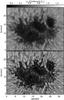 |
Fig. 1 Stokes I continuum intensity of the Hinode/SP map of a sunspot umbra of NOAA AR 10933. The original data are plotted in the top panel. The Stokes I continuum resulting from the 2D inversion is shown in the bottom panel. The intensity is normalized to the mean quiet-Sun intensity IQS. The outer contour line in the bottom panel indicates the edge of the umbra as retrieved from the magnetic field inclination map (see main text), the inner contour line separates central from peripheral umbral dots (UDs). Four typical UDs are marked by circles and letters. |
Under the assumption of local thermodynamic equilibrium, the Stokes profiles of the Fe i 6301.5 Å and 6302.5 Å lines were inverted by applying the version of the SPINOR inversion code (Frutiger 2000; Frutiger et al. 2000) extended by van Noort (2012). In this version of the code, the instrumental effects responsible for the spectral and spatial degradation of the observational data are taken into account, so that the inverted parameters correspond to spatially deconvolved values (but without the added noise that deconvolution generally introduces). The observational data are spatially upsampled by a factor of two, so that the input and output data of the SPINOR inversion have a sampling of 0.′′08 per pixel (for details, see van Noort et al. 2013). According to van Noort (2012), the spatial PSF used for the inversion considers the 0.5 m clear aperture of the SOT, the central obscuration, the spider (Tsuneta et al. 2008; Suematsu et al. 2008), and a defocus of 0.1 waves, even though the focus position of our data set was not accurately known. Height-dependent temperature, line of sight (LOS) velocity, magnetic field strength, field inclination, field azimuth, and micro-turbulence are determined at three log τ500 nodes: − 2.5, − 0.9, and 0. More details of the inversion of this spot are provided in van Noort et al. (2013) and Tiwari et al. (2013).
A continuum map obtained from the best-fit Stokes I profiles of the 2D inversion result can be seen in the bottom panel of Fig. 1. Since the deconvolution of the data with the theoretical spatial PSF is now indirectly part of the inversion process, the contrast is significantly enhanced and UDs can be identified much more clearly than in the original data. Hence, the continuum map in the bottom panel of Fig. 1 was used for a manual detection of the location of the most prominent 67 UDs. Misidentification of brightness features that are separated from the penumbra in the continuum image but are still connected to the penumbra in the magnetic field inclination map were excluded since we defined the boundary of the umbra by thresholding the lowpass-filtered inclination map (7 × 7 pixels) at 40 degrees and corrected the boundary found in this way manually in a few doubtful cases where the penetration of long and narrow penumbral filaments led to a wrong result. The umbral boundary is shown as the outer contour line in the bottom panel of Fig. 1. Furthermore, we divided the set of 67 UDs into 23 central UDs (CUDs) and 44 peripheral UDs (PUDs). The inner contour line in the bottom panel of Fig. 1 separates the PUDs from the CUDs. The criterion used is simply the distance to the umbra-penumbra boundary. CUDs are >1000 km away from this boundary, PUDs ≤1000 km.
Once the locations of the UDs’ centers were known, the UD boundaries were determined from the continuum map by a multilevel tracking (MLT) algorithm (see Bovelet & Wiehr 2001), using 25 equidistant intensity levels. The resulting contiguous MLT structures were then cut at 50% of the local min-max intensity range, which was taken as the UD boundary. A detailed description of the use of the MLT algorithm for isolating UDs is given in Riethmüller et al. (2008b).
The knowledge of the UD boundaries allowed us to average UD properties over all pixels within the UD boundary. Stratifications of temperature, LOS velocity, and field strength of the UDs were then determined as such averages. The same quantities were also determined for the UDs’ diffuse background (DB), defined as the average over all pixels (ignoring penumbral pixels) in a 400-km-wide ring around the UD boundary. UD and DB quantities were retrieved for optical depths between log τ500 = − 2.5 and 0 in steps of 0.5.
The LOS velocity maps of the inversion result show a clear p-mode pattern with a spatial wavelength of about 10′′ that has to be removed to avoid any p-mode influence on our results. The usually employed technique of Fourier filtering in 3D kω-space cannot be applied in our case because only a single map of the observational data was available for inversion. We therefore removed the p-modes in the LOS velocity maps at all used log τ500 nodes by applying a highpass filter (implemented as the difference between the original velocity map and its running boxcar, 21 × 21 pixels, filtered counterpart). Since our results depend on a careful zero-velocity determination, we re-calibrated the velocities even if the highpass filter already roughly removed the velocity offset. To achieve this we assumed that the dark core of the umbra is at rest. The darker part of the umbra is identified by thresholding the lowpass-filtered continuum image (11 × 11 pixels) at 50% of the intensity range. We furthermore excluded a circle of 500 km radius around each of the 67 identified UDs and subtracted the mean velocity of the remaining dark umbral pixels from the velocity maps at each optical depth. This procedure was found to be robust in the sense that changing the threshold for identifying the darkest part of the umbra by ±10%, or increasing the radius of the exclusion zone around the UDs by 200 km, did not influence our results.
3. Results
Even at the significantly improved image quality provided by the inversion, we were unable to find dark lanes in the central parts of the UDs as reported in Schüssler & Vögler (2006) in MHD simulations and in Bharti et al. (2007) in other deconvolved Hinode images.
The stratifications of temperature, velocity, and field strength, averaged separately over all PUDs and CUDs, are displayed in Fig. 2. While in the upper photosphere (log τ500 = − 2.5) the considered properties hardly differ between the mean UD and DB, they deviate significantly from each other in the deep photosphere (log τ500 = 0). Compared with their DB, we find a temperature enhancement and field-weakening of 610 K and 580 G at optical-depth unity for the mean PUD, while for CUD the values are 570 K and 530 G. The mean UD magnetic field weakens with depth, while the field strength of the mean DB increases with depth, as expected.
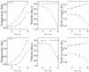 |
Fig. 2 Optical-depth dependence of temperature, LOS velocity, and magnetic field strength averaged over 44 peripheral umbral dots (top three panels) and 23 central umbral dots (bottom three panels). The error bars denote standard deviations of the mean (σ/ |

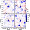 |
Fig. 3 LOS velocities at optical-depth unity of typical UDs marked as circles of 200 km radius around the position of the UD’s peak intensity. The UDs in the center of each panel identified by letters are the same as in the bottom panel of Fig. 1. |
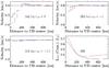 |
Fig. 4 Panels a)–c): LOS velocity at constant optical depth as function of the distance to the UD center averaged over all azimuthal angles of the peripheral (red lines) and central (blue lines) UDs. The optical depths are given as text labels. Panel d): mean continuum intensity profile of the two UD classes. |
Upward and downward mass fluxes per umbral dot (computed within 500 km radii) and their ratios at various optical depths.
The LOS velocity (which is virtually identical to the vertical velocity component due to the small heliocentric angle) of DB and UD is almost zero in the upper photosphere. Strong upflows of − 900 m/s and − 720 m/s are found at optical-depth unity for the mean PUD and CUD, while a weak but significant downflow of 57 m/s is found for the mean DB of the peripheral UDs only. These values should be compared with the uncertainty in the velocity averaged over the DB of PUDs,  m/s (σ – standard deviation of the 44 DB velocities from their mean value, N = 44 – number of UDs). The DB of the central UDs is on average at rest within the error bars. A better insight into the up- and downflows in and around UDs is given in Figs. 3 and 4. The LOS velocity maps at log τ500 = 0 are shown in Fig. 3 for four typical UDs and reveal that the upflows are mainly concentrated within the marked 200 km vicinity of the UD center, while weaker downflows are preferentially found farther out. In general, the downflows only partly surround a UD, they are often concentrated on one or two sides of the UD. Although weak upflows are also present in the vicinities of UDs, the downflows dominate for the PUDs, as deduced from Figs. 2 and 4. For a better visibility the spatial sampling of the maps was increased via bi-linear interpolation.
In Fig. 4, we averaged the velocities of all pixels within rings of 40 km width around the UD center (ignoring penumbral pixels) and plotted the mean velocities as a function of the distance to the UD’s center, again separately for PUDs and CUDs. Note that this method is independent of any determination of the UD boundary. Panel a of Fig. 4 shows the velocities at optical-depth unity. Between 0–200 km distance from the UD’s center, we find upflows (see enlarged velocity maps in Fig. 3 where the UDs are marked with circles having a 200 km radius). Then, from 200 to 500 km we see downflows (between 200 and 350 km for CUDs), while for distances larger than 500 km the velocity is almost zero. The downflows in the lower photosphere peak at a distance of roughly 240 km from the UD’s center and have values of 110 m/s and 58 m/s for the mean PUD and CUD. They are thus minute compared to the maximum upflows in the UDs of − 960 m/s and − 600 m/s. The upflows and downflows are on average stronger for the PUDs than for the CUDs. Both up- and downflows increase rapidly with depth (compare panels a–c). The upflows within the UDs are much weaker at log τ500 = − 1 (panel b) and the downflows cannot be seen anymore. At log τ500 = − 2.5 (panel c), there is almost no velocity signal. The mean intensity profiles are plotted in panel d and reveal a half-width-half-maximum radius of 120 km for the PUDs and 140 km for the CUDs.
We next calculated mass fluxes as the sum over all pixels within a 500-km vicinity of the UD center since for larger distances the velocity is negligible. The required densities were provided by the SPINOR code under the assumption of hydrostatic equilibrium. Table 1 lists the upward and downward mass fluxes per UD, Mu, and Md for various optical depths and separately for the two UD classes. The uncertainties in Table 1 are the standard deviations of the averages over all UDs of a given class (σ). The last two columns give the mass flux ratios. The mass flux increases strongly with depth due to the density and velocity increase. Even if the method of azimuthal averaging leads to downflow velocities that are lower than the upflow velocities, the averaging is performed over a much larger area so that the upward and downward mass flux are roughly balanced within the uncertainties.
4. Discussion and conclusions
We have used a new inversion technique to retrieve the atmospheric parameters of 67 UDs in a sunspot umbra from data recorded with the spectropolarimeter onboard Hinode. In agreement with earlier studies (Socas-Navarro et al. 2004; Riethmüller et al. 2008a), we found that in the deep photosphere the temperature is enhanced and the magnetic field is weakened in the UDs compared with their umbral surroundings. Table 2 compares the main UD properties retrieved from the conventional and the improved inversion technique. For a direct comparison with Riethmüller et al. (2008a), who reported peak values and not spatial averages, we also listed the peak values obtained from the new inversion in Table 2. In fact, all values listed in Table 2 are higher for the new inversion method, which emphasizes the considerably improved data quality reached by the implicit removal of the telescope’s spatial PSF.
Comparison of UD properties at the continuum formation height between Riethmüller et al. (2008a) and this study.
The 2D inversion results revealed clear upflow signals for both UD types, while Riethmüller et al. (2008a) could only find them for the PUDs. On average, UDs show upflows up to a radial distance of 200 km from their centers. In general, these upflows are stronger for PUDs than for CUDs. Between 200 and 500 km from a UD’s center, we found low but significant downflows, whereas there is no relevant velocity signal farther away. The velocity signal decreases rapidly with atmospheric height.
Previous observational studies detected upflows, but could not detect downflows associated with UDs (e.g. Socas-Navarro et al. 2004; Riethmüller et al. 2008a; Watanabe et al. 2012), or at least not systematically (Ortiz et al. 2010). This raised the question where all the upflowing plasma ends up. The first systematic detection of downflows around UDs in this paper gives us the possibility of calculating upward and downward mass fluxes. Our finding of the very well-balanced mass fluxes depends on the careful velocity calibration described in Sect. 2. If all umbral pixels had been used for the zero velocity determination, the zero velocity could possibly be blueshifted due to the UD upflows, thus giving rise to artificial downflows. This effect is ruled out since our velocity re-calibration ignores the UDs and uses the darkest parts of the umbra only.
We furthermore believe that the downflows seen in the top left panel of Fig. 4 are real and not a result of ringing effects. Such effects could be caused by the nearly axisymmetrical shape of the spatial PSF used in our inversion and would have affected all quantities. However, plots of temperature and field strength versus the UD center distance (not shown) do not exhibit any signs of ringing. According to Schüssler & Vögler (2006), the downflows are concentrated in narrow channels preferentially at the endpoints of the central dark lanes of the UDs. Our spatial resolution is insufficient to detect the dark lanes or the narrow downflow channels. The relatively weak downflow signals become significantly stronger than the noise only after the azimuthal averaging around UDs.
The picture introduced in Schüssler & Vögler (2006) of UDs as a natural consequence of magnetoconvection in the strong vertical magnetic field of an umbra is qualitatively confirmed by our study. In deep layers the rising hot plasma pushes the field to the side, weakening the field there. Around the continuum formation height the rising gas cools through radiative losses, turns over, and flows down around the UDs. This evidence for overturning comes from the mass balance between up- and downflows and from the fact that the central upflows are associated with hot material, whereas the peripheral downflows are cool. Furthermore, the rapid decrease of upward mass flux with height is also typical for overturning, overshooting convection. The fact that PUDs are associated with higher flow velocities and slightly higher temperature enhancements suggests a more vigorous convection than in the central umbra. We note, however, that our results differ in one detail from the simulations. Whereas the simulations produce concentrated downflows on opposite ends of the UDs, the observations reveal a more diffuse downflow structure.
The 2D inversion technique also returns an enhanced temperature excess and magnetic-field reduction compared with traditional inversions. The temperature and magnetic field anomalies turn out to be very similar for PUDs and CUDs (within 10% of each other).
We suggest observations at a spatial resolution higher than available here, e.g., with the re-flight of the 1 m Sunrise telescope (Solanki et al. 2010; Barthol et al. 2011), or with the envisaged 1.5-m Solar-C telescope, to determine if the UDs show the predicted central dark lanes with narrow downflow channels at their endpoints.
Acknowledgments
Hinode is a Japanese mission developed and launched by ISAS/JAXA, with NAOJ, NASA, and STFC (UK) as partners. This work has been partly supported by the WCU grant No. R31-10016 funded by the Korean Ministry of Education, Science & Technology.
References
- Adjabshirzadeh, A., & Koutchmy, S. 1983, A&A, 122, 1 [NASA ADS] [Google Scholar]
- Barthol, P., Gandorfer, A., Solanki, S. K., et al. 2011, Sol. Phys., 268, 1 [NASA ADS] [CrossRef] [Google Scholar]
- Bharti, L., Joshi, C., & Jaaffrey, S. N. A. 2007, ApJ, 669, L57 [NASA ADS] [CrossRef] [Google Scholar]
- Bharti, L., Beeck, B., & Schüssler, M. 2010, A&A, 510, A12 [NASA ADS] [CrossRef] [EDP Sciences] [Google Scholar]
- Biermann, L. 1941, Vierteljahrsschr. Astron. Ges., 76, 194 [Google Scholar]
- Borrero, J. M., & Ichimoto, K. 2011, Liv. Rev. Sol. Phys., 8, 4 [Google Scholar]
- Bovelet, B., & Wiehr, E. 2001, Sol. Phys., 201, 13 [NASA ADS] [CrossRef] [Google Scholar]
- Chevalier, S. 1916, Ann. Obs. Astron. Zô-Sè, Tome IX, Plate XIV & Page B29 [Google Scholar]
- Frutiger, C. 2000, Ph.D. Thesis, Institute of Astronomy, ETH Zürich [Google Scholar]
- Frutiger, C., Solanki, S. K., Fligge, M., & Bruls, J. 2000, A&A, 358, 1109 [NASA ADS] [Google Scholar]
- Kosugi, T., Matsuzaki, K., Sakao, T., et al. 2007, Sol. Phys., 243, 3 [NASA ADS] [CrossRef] [Google Scholar]
- Lites, B. W., Elmore, D. F., & Streander, K. V. 2001, in Advanced Solar Polarimetry, ed. M. Sigwarth (San Francisco: ASP), ASP Conf. Ser., 236, 33 [Google Scholar]
- Louis, R. E., Mathew, S. K., Bellot Rubio, L. R., et al. 2012, ApJ, 752, 109 [NASA ADS] [CrossRef] [Google Scholar]
- Ortiz, A., Bellot Rubio, L. R., & Rouppe van der Voort, L. 2010, ApJ, 713, 1282 [NASA ADS] [CrossRef] [Google Scholar]
- Riethmüller, T. L., Solanki, S. K., & Lagg, A. 2008a, ApJ, 678, L157 [NASA ADS] [CrossRef] [Google Scholar]
- Riethmüller, T. L., Solanki, S. K., Zakharov, V., & Gandorfer, A. 2008b, A&A, 492, 233 [NASA ADS] [CrossRef] [EDP Sciences] [Google Scholar]
- Rimmele, T. 2008, ApJ, 672, 684 [NASA ADS] [CrossRef] [Google Scholar]
- Schüssler, M., & Vögler, M. 2006, ApJ, 641, L73 [NASA ADS] [CrossRef] [Google Scholar]
- Sobotka, M. 2006, Diss. for Doctor Scientiarum, Acad. Sci. Czech Republic [Google Scholar]
- Socas-Navarro, H., Martínez Pillet, V., Sobotka, M., & Vázquez, M. 2004 ApJ, 614, 448 [Google Scholar]
- Solanki, S. K. 2003, A&ARv, 11, 153 [Google Scholar]
- Solanki, S. K., Barthol, P., Danilovic, S., et al. 2010, ApJ, 723, L127 [NASA ADS] [CrossRef] [Google Scholar]
- Suematsu, Y., Tsuneta, S., Ichimoto, K., et al. 2008, Solar Phys., 249, 197 [Google Scholar]
- Tiwari, S. K., van Noort, M., Lagg, A., & Solanki, S. K. 2013, A&A, submitted [Google Scholar]
- Tsuneta, S., Ichimoto, K., Katsukawa, Y., et al. 2008, Sol. Phys., 249, 167 [NASA ADS] [CrossRef] [Google Scholar]
- van Noort, M. 2012, A&A, 548, A5 [NASA ADS] [CrossRef] [EDP Sciences] [Google Scholar]
- van Noort, M., Lagg, A., Tiwari, S. K., & Solanki, S. K. 2013, A&A, submitted [Google Scholar]
- Watanabe, H., Bellot Rubio, L. R., de la Cruz Rodríguez, J., & Rouppe van der Voort, L. 2012, ApJ, 757, 49 [NASA ADS] [CrossRef] [Google Scholar]
- Weiss, N. O. 2002, Astron. Nachr., 323, 371 [NASA ADS] [CrossRef] [Google Scholar]
All Tables
Upward and downward mass fluxes per umbral dot (computed within 500 km radii) and their ratios at various optical depths.
Comparison of UD properties at the continuum formation height between Riethmüller et al. (2008a) and this study.
All Figures
|
Fig. 1 Stokes I continuum intensity of the Hinode/SP map of a sunspot umbra of NOAA AR 10933. The original data are plotted in the top panel. The Stokes I continuum resulting from the 2D inversion is shown in the bottom panel. The intensity is normalized to the mean quiet-Sun intensity IQS. The outer contour line in the bottom panel indicates the edge of the umbra as retrieved from the magnetic field inclination map (see main text), the inner contour line separates central from peripheral umbral dots (UDs). Four typical UDs are marked by circles and letters. |
| In the text | |
|
Fig. 2 Optical-depth dependence of temperature, LOS velocity, and magnetic field strength averaged over 44 peripheral umbral dots (top three panels) and 23 central umbral dots (bottom three panels). The error bars denote standard deviations of the mean (σ/ |
| In the text | |
|
Fig. 3 LOS velocities at optical-depth unity of typical UDs marked as circles of 200 km radius around the position of the UD’s peak intensity. The UDs in the center of each panel identified by letters are the same as in the bottom panel of Fig. 1. |
| In the text | |
|
Fig. 4 Panels a)–c): LOS velocity at constant optical depth as function of the distance to the UD center averaged over all azimuthal angles of the peripheral (red lines) and central (blue lines) UDs. The optical depths are given as text labels. Panel d): mean continuum intensity profile of the two UD classes. |
| In the text | |
Current usage metrics show cumulative count of Article Views (full-text article views including HTML views, PDF and ePub downloads, according to the available data) and Abstracts Views on Vision4Press platform.
Data correspond to usage on the plateform after 2015. The current usage metrics is available 48-96 hours after online publication and is updated daily on week days.
Initial download of the metrics may take a while.