| Issue |
A&A
Volume 554, June 2013
|
|
|---|---|---|
| Article Number | A101 | |
| Number of page(s) | 22 | |
| Section | Celestial mechanics and astrometry | |
| DOI | https://doi.org/10.1051/0004-6361/201220748 | |
| Published online | 11 June 2013 | |
Dynamical analysis of nearby clusters⋆
Automated astrometry from the ground: precision proper motions over a wide field
1 Centro de Astrobiología, depto de Astrofísica, INTA−CSIC, PO BOX 78, 28691, ESAC Campus, 208691 Villanueva de la Cañada, Madrid Spain
e-mail: This email address is being protected from spambots. You need JavaScript enabled to view it.
2 Institut d’Astrophysique de Paris, CNRS UMR 7095 and UPMC, 98bis bd Arago, 75014 Paris, France
3 UJF-Grenoble 1/CNRS−INSU, Institut de Planétologie et d’Astrophysique de Grenoble (IPAG), UMR 5274, 38041 Grenoble, France
4 Canada − France − Hawaii Telescope Corporation, 65-1238 Mamalahoa Highway, Kamuela, HI 96743, USA
5 Calar Alto Observatory, Centro Astronómico Hispano Alemán, Calle Jesús Durbán Remón, 04004 Almería, Spain
6 European Southern Observatory, Alonso de Cordova 3107 Vitacura, Santiago, Chile
Received: 16 November 2012
Accepted: 18 April 2013
Abstract
Context. The kinematic properties of the different classes of objects in a given association hold important clues about the history of its members, and offer a unique opportunity to test the predictions of the various models of stellar formation and evolution.
Aims. DANCe (standing for dynamical analysis of nearby clusters) is a survey program aimed at deriving a comprehensive and homogeneous census of the stellar and substellar content of a number of nearby (<1 kpc) young (<500 Myr) associations. Whenever possible, members will be identified based on their kinematics properties, ensuring little contamination from background and foreground sources. Otherwise, the dynamics of previously confirmed members will be studied using the proper motion measurements. We present here the method used to derive precise proper motion measurements, using the Pleiades cluster as a test bench.
Methods. Combining deep wide-field multi-epoch panchromatic images obtained at various obervatories over up to 14 years, we derived accurate proper motions for the sources in the field of the survey. The datasets cover ≈80 square degrees, centered around the Seven Sisters.
Results. Using new tools, we have computed a catalog of 6 116 907 unique sources, including proper motion measurements for 3 577 478 of them. The catalog covers the magnitude range between i = 12 ~ 24 mag, achieving a proper motion accuracy <1 mas y-1 for sources as faint as i = 22.5 mag. We estimate that our final accuracy reaches 0.3 mas yr-1 in the best cases, depending on magnitude, observing history, and the presence of reference extragalactic sources for the anchoring onto the ICRS.
Key words: astrometry / proper motions / stars: kinematics and dynamics
Based on observations obtained with MegaPrime/MegaCam, a joint project of CFHT and CEA/DAPNIA, at the Canada-France-Hawaii Telescope (CFHT) which is operated by the National Research Council (NRC) of Canada, the Institut National des Science de l’Univers of the Centre National de la Recherche Scientifique (CNRS) of France, and the University of Hawaii.
© ESO, 2013
1. Introduction
The Milky Way galaxy includes large-scale structures such as clusters, star-forming regions, and OB associations. Understanding the formation, structure, and evolution of these components has been one of the greatest challenges of modern astrophysics. Following the advent of sensitive wide-field instruments over the past two decades, a large number of photometric studies have been performed in stellar associations and clusters (e.g. Knödlseder 2000; Barrado y Navascués et al. 2004; Béjar et al. 2001; Lodieu et al. 2006; Torres et al. 2008; Eiroa & Casali 1992). These surveys not only dramatically improved our knowledge of the luminosity function, but also extended it to the substellar and planetary mass regimes. They nevertheless suffer from several limitations, making their comparison with theoretical predictions sometimes difficult. Any photometric selection indeed relies on theoretical tracks, and hence age estimates that are still uncertain at young ages (Baraffe et al. 2009). Additionally, the photometric variability inherent to their youth can affect their luminosity and colors, leading to a significant fraction of missed members. Foreground stars and extragalactic sources will in most cases be a major source of contamination. Finally, photometric surveys are not able to distinguish members of neighboring or spatially coincident groups, possibly leading to confusion and erroneous conclusions regarding their origin. Selecting members based on their kinematics offers several advantages: it is completely independant of evolutionary models; it rejects the majority of unrelated foreground and background sources; it is insensitive to variability or flux excess and deficiency related to, e.g., circumstellar material or accretion; it can separate coincident or neighboring associations provided that they have differing mean motions (e.g. σ-Ori, Lupus, and Upper Scorpius, Jeffries et al. 2006; Brandner et al. 1996; Köhler et al. 2000; Kraus & Hillenbrand 2007; López Martí et al. 2011).
The study of kinematics involves two complementary observational techniques: radial and transverse velocity measurements. Systematic radial velocity surveys over extended (>10 deg2) regions of the sky require large amounts of telescope time. The most succesful and efficient spectroscopic surveys to date (e.g. RAVE, WOCS, APOGEE, MARVELS, ESO-Gaia, Steinmetz et al. 2006; Mathieu 2000; Majewski et al. 2007; Mahadevan et al. 2007; Gilmore et al. 2012) are producing libraries that include several hundreds of thousands of high-quality spectra and radial velocity measurements over areas as large as several thousands square degrees. They are nevertheless still limited to the brightest sources and do not reach the substellar luminosity range. Proper motion measurements are, on the other hand, much easier to achieve. One in principle only needs two observations separated by a sufficient period of time. A number of nearby associations have mean proper motions of a few tens of mas yr-1 (e.g. Pleiades, Hyades, Taurus, and Ophiuchus, Kharchenko et al. 2005; Bobylev 2006) which facilitates measuring their members’ motion over a few years only. In spite of the tremendous efforts conducted over the past 20 yr, the limited sensitivity of the various large-scale kinematics projects has restricted the study to the solar neighborhood (e.g. Hipparcos) or to the identification of nearby moving groups (Torres et al. 2006, 2008; Zuckerman et al. 2004, 2001, 2006). Local kinematics has been commonly used to confirm photometrically selected samples (see e.g. Moraux et al. 2001, 2003; Kraus & Hillenbrand 2007; Lodieu et al. 2007a,b, 2012; Gálvez-Ortiz et al. 2010; López Martí et al. 2011), but kinematically selected samples over large areas of young nearby associations are still sorely lacking.
The future Gaia space mission (Perryman et al. 2001) will provide an exquisite accuracy and complete six-dimension census of the sky up to G ≈ 15 mag, and a five-dimension census up to G ≈ 20 mag. Although it represents a tremendous improvement with respect to its predecessor Hipparcos (Perryman et al. 1997), Gaia will unfortunately not be sensitive enough to study the least massive objects. G ≈ 20 mag indeed corresponds to ≈15 MJup at 150 pc and for an age of 1 Myr (Baraffe et al. 1998), when the mass function is known to extend at least to 3 ~ 4 MJup (e.g. Bayo et al. 2011,and references therein). Additionally, young stellar clusters and associations are very often deeply embedded and contain bright H II regions. Since it will operate in the visible part of the spectrum, Gaia will be mostly blind in regions of heavy extinction and bright nebular emission, precisely where most of the star formation is taking place.
Recently, Anderson et al. (2006) demonstrated that high-precision astrometry could be extracted from wide-field ground-based CCD images, and studied extended areas around galactic globular clusters (Bellini et al. 2009; Bellini & Bedin 2010; Yadav et al. 2008) using observations obtained with the ESO WFI wide-field camera. In this paper, we present a similar method designed to automatically process and analyze vast amounts of images (several thousands) originating from multiple instruments and sites and covering large (>10 deg2) areas of the sky.
2. The DANCe project
Taking advantage of the wide-field surveys performed in the early 2000, we are performing a comprehensive study of kinematics in a number of nearby (≲1 kpc) associations and clusters. A preliminary list of targets with publicly available archival observations is given in Bouy et al. (2011), and we are welcoming suggestions and proposals of collaborative studies for other associations and clusters of particular interest. The initial surveys reached sensitivities well beyond the substellar limit at the age and distance of these associations. Complementing these archival data with new sensitive wide-field observations, we are compiling a multi-epoch panchromatic database encompassing large (several tens of square degrees) areas of young nearby associations. This database is used to derive accurate proper motions for all sources with multi-epoch detections. The scientific goals of the DANCe project are twofold:
-
mass function: when the association mean proper motion allowsit, the proper motion and accurate photometric measurementscan be used to select members and/or reject contaminants andderive more accurate luminosity (mass) functions. The samplescan be used to study the stellar content within each groupseparately, and to perform a meaningful intercomparisonbetween groups of various ages, structures, metallicities, anddensities.
-
internal dynamics: the observed velocity distribution of confirmed members and its dependance on stellar mass, spatial distribution, and environment can be compared with advanced N-body numerical simulations and dynamical evolution models (Adams 2001; Proszkow & Adams 2009; Marks & Kroupa 2012). Ultimately, complementary radial velocity measurements can provide a complete picture of the space motions within young associations, below the substellar limit.
3. Test case: the Pleiades
Their youth and proximity have made the Pleiades one of the most extensively studied clusters over the past hundred years. In their recent review of the cluster, Stauffer et al. (2007) and Lodieu et al. (2012) have compiled an exhaustive list of candidate and confirmed members originating from more than a dozen independent surveys of the Pleiades. The total number of members and candidate members reported in their catalogs adds up to 1471 objects. The relatively large mean proper motion of the group and the vast amounts of images available in public archives makes it an ideal target to develop the large-scale data processing and automatic astrometric algorithms presented in this manuscript.
4. Archival data
In an effort to compile the most complete dataset − both in terms of spatial and time coverage − we searched the Subaru Telescope, the Isaac Newton Telescope (INT), the United Kingdom Infrared Telescope (UKIRT), the Cerro Tololo Inter-American Observatory (CTIO, at NOAO), the Kitt Peak National Observatory (KPNO, at NOAO), the Canada France Hawai’i Telescope (CFHT), and the European Southern Observatory (ESO) public archives for wide-field images within a box of 10° × 10° centered on the Pleiades. Figure 1 and Table 1 give an overview of the properties and coverage of the various datasets and instruments. The filter sets used for these observations are described in Fig. 21. The data were obtained with nine different instruments at five observatories. A summary of their characteristics is given in the following sections.
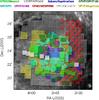 |
Fig. 1 IRAS 100 μm image of the Pleiades cluster with the various surveys used in this study overplotted. The Seven Sisters are represented with yellow stars. The full Moon is represented in the lower right corner to illustrate the scale. |
-
CFH Telescope: The CFH12K (Cuillandre et al. 2000) and UH8K (Metzger et al. 1995) observations of the Pleiades are described in detail in Bouvier et al. (1998), Moraux et al. (2001), and Moraux et al. (2003). The MegaCam (Boulade et al. 2003) observations are described in Sect. 5. The individual images were processed and calibrated with the recommended Elixir system (Magnier & Cuillandre 2004), which includes detrending (darks, biases, flats, and fringe frames), and astrometric registration. Nightly magnitude zero-points were derived by the CFHT team using standard-star fields (Landolt 1992).
-
Subaru Telescope: The Suprime-Cam (Miyazaki et al. 2002) images were processed (overscan subtraction, flat-fielding, and masking of vignetted areas) using the recommended SDFRED1 package (Ouchi et al. 2004; Yagi et al. 2002) and the relevant calibration frames obtained the same night. The photometric conditions on Mauna Kea were poor during these observations, as described in the Skyprobe database (Cuillandre et al. 2004). We therefore did not attempt to calibrate the corresponding photometry.
-
INT Telescope: We retrieved the detrended individual Wide-Field Camera (WFC, Ives 1998) images from the ING public archive. About 88% of these observations were obtained under photometric ambient conditions, as described by the INT data quality control system, and the nightly photometric zeropoints provided by the ING were applied.
-
UKIRT Telescope: The cluster was observed in the near-infrared (near-IR) with the Wide-Field CAMera (WFCAM, Casali et al. 2007) in the course of the UKIRT InfraRed Deep Sky Surveys (UKIDSS, Lawrence et al. 2007). The UKIDSS survey provides a homogeneous coverage of the association in the Z, Y, J, H, and Ks filters. The UKIDSS release (DR9) includes observations performed between September 2005 and January 2011; they and are described in Lodieu et al. (2007a) and Lodieu et al. (2012). We noticed that the point spread function (PSF) of the pipeline processed interleaved images was not optimal for an accurate astrometric analysis. We therefore retrieved the individual frames from the WFCAM Science Archive (Hambly et al. 2008). These frames are flat-fielded, dark-subtracted, and sky-subtracted, and include an approximate astrometric solution with an accuracy better than a few arcsec. After extracting the sources from these individual images, a photometric calibration was derived using the UKIDSS catalog.
-
KPNO Mayall Telescope: We searched and retrieved NOAO Extremely Wide-Field Infrared Imager (NEWFIRM) (Autry et al. 2003) and MOSAIC-1 (Wolfe et al. 2000) images in the NOAO Science Archive. The MOSAIC1 images were processed following standard procedures using the mscred package within IRAF2 and the relevant calibration frames, as recommended in the user manual. The detrended and sky-subtracted NEWFIRM images and their respective confidence maps were retrieved from the NOAO archive (Swaters et al. 2009). The NEWFIRM J-band photometry was then tied to the UKIDSS one.
-
CTIO Blanco Telescope: MOSAIC2 is a clone instrument of the MOSAIC1 installed on the Blanco telescope at CTIO. We retrieved the raw images from the NOAO Science Archive, and processed them following standard procedures using the mscred package within IRAF and the relevant calibration frames, as recommended in the user manual.
Although in most cases sets of several consecutive and dithered images were obtained, we chose to perform the analysis on the individual images rather than on stacks. While individual images do not go as deep as stacks, this choice ensures that the PSF (and hence the astrometric accuracy) and noise are not affected by the stacking process. As we will see, using individual images offers other advantages, in particular, a more efficient rejection of problematic frames or measurements, and an opportunity to reach out for faster-moving objects.
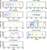 |
Fig. 2 Transmission of the various filters used in this study. In the z-band, the sensitivity is limited by the CCD quantum efficiency, which typically drops at 900 ~ 1000 nm. |
5. New observations
To complement the archival data and increase both the time baseline and spatial coverage, we obtained deep wide-field images of the cluster with MegaCam at the CFHT. The observations were designed to optimize the astrometric calibration. The various pointings were chosen to overlap by a few arcminutes, ensuring an accurate astrometric anchoring over the entire survey. Each pointing was obtained in dither mode, with a dither width of a few arcminutes. This dithering allows filling the CCD-to-CCD gaps and correcting for deviant pixels and cosmic-ray events, and helps deriving an accurate astrometric solution over the entire field-of-view (see Sect. 7.6). The nights were photometric, with an average seeing full-width at half maximum (FWHM) in the range 0 5–07 as measured in the images. The data were processed and calibrated with the recommended Elixir system, and the nightly magnitude zero-points measured by the CFHT team were applied.
6. Observation properties
Describing the properties of every single individual image used in this study woud be impractical. Instead, we present general statistics of three observational properties especially important for the purpose of our study: airmass, image FWHM, and sensitivity. The latter two are important parameters because the best positional accuracy achievable is mostly limited by the signal-to-noise ratio (S/N) (hence sensitivity), the FWHM of the point sources, and the sampling (pixel scale) of the images (King 1983). The airmass is playing an important role as well, as atmospheric turbulence and differential chromatic refraction quickly increase with airmass. Figure 3 shows the distribution of airmass for the observations used in this study. About 75% of the observations were obtained at airmass <1.2, and ≈90% at airmass <1.3. It also shows the distribution of the FWHM measured for all individual unresolved detections (point sources). About two thirds have  , and about 92% have FWHM ≤ 1″. Finally, even though the sensitivity of the individual frames varies greatly, the various observations routinely reached luminosities fainter than 22 mag in the optical (λ < 1.0 μm), and 18 mag in the near-IR (λ > 1.0 μm).
Whenever we could assess that an observation had been performed under good photometric conditions and that an absolute photometric calibration (photometric standard field) was available, we applied the corresponding zero-point to the photometry extracted by SExtractor. The associated absolute photometric uncertainties are typically about 5 ~ 10%. Most of the photometric measurements (all except the Subaru/SuprimeCam, CTIO/MOSAIC2, KPNO/MOSAIC1 and some INT/WFC) were obtained under clear or photometric conditions.
Instruments and references to the corresponding surveys.
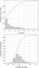 |
Fig. 3 Upper panel: distribution of airmass for the observations. Lower panel: distribution of FWHM of all the individual unresolved detections. The lines represents the cumulative distribution. |
7. Astrometric analysis
The astrometric analysis involves vast amounts of multi-epoch, multi-instrument, multi-wavelength datasets, and requires highly automatized tools; all our processing is performed with the AstrOmatic3 software suite (Bertin 2010). The whole process is decomposed into the following steps, which we describe in detail in the next sections:
-
1.
Recovering and equalizing image metadata.
-
2.
Modeling the PSF.
-
3.
Cataloging.
-
4.
Quality assurance.
-
5.
Estimating astrometric uncertainties.
-
6.
Computing a global astrometric solution.
-
7.
Robust fitting of individual source proper motions.
7.1. Recovering and equalizing image metadata
The PSF modeling, source extraction, and astrometric calibration tasks rely on a handful of parameters that must be set before processing the data. These parameters comprise detector gains, saturation levels, the approximate position and scale of the pixel grids on the sky, dates and times of observation, durations of exposure, airmass, filter-wheel position and instrumental setups that define the instrumental context for the astrometric solution (see Sect. 7.6).
Recovering and uniformizing these parameters proves to be a laborious undertaking; one faces here not one but nine different mosaic instruments over many years of operation. In practice, and despite decades of effort from the community to promote the standardization of metadata description in FITS headers, each instrument uses slightly different conventions, which often evolve during the life of the instrument. Among all parameters, the detector saturation level (required for excluding saturated sources from the PSF modeling process and from the astrometric solution) was found the least reliable. It was often overestimated, and on one occasion it would ignore a scaling factor applied to the data, a problem that also plagued the gains. Because of this, we ended up using S/N-vs-SPREAD_MODEL diagrams (see Sect. 7.4) to correct individual detector saturation levels.
7.2. Modeling the point spread function with PSFEx
The first step in making precise measurements of the positions of individual sources is to compute an accurate model of the (variable) PSF for every chip of every exposure. A large fraction of the images (those with good seeing) are significantly undersampled with some of the instruments, especially WFCam and Mosaic2. This requires the PSF to be modeled at the sub-pixel level. The PSFEx software (Bertin 2011) has been specifically designed to work with undersampled images and arbitrary PSF shapes. Briefly, PSFEx fits the image of every point-source ps with a projection on the local pixel grid of the linear combination of basis vectors φb by minimizing the χ2 function of the coefficient vector c (1)where
  is the PSF model sampled at the location of star s:
 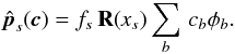 (2)fs is the flux within some reference aperture, and Ws the inverse of the pixel noise covariance matrix for point-source s. We assume that Ws is diagonal. R(xs) is a resampling operator that depends on the image grid coordinates xs of the point-source centroid:
  (3)where h is a 2D interpolant (interpolating function), xi is the coordinate vector of image pixel i, xj the coordinate vector of model sample j, and η is the image-to-model sampling step ratio (oversampling factor). We adopt a Lanczós-4 function (Duchon 1979) as interpolant. PSFEx is able to model smooth PSF variations within each chip by expanding the set of unknowns in (Eq. (2)) as a linear combination of polynomial functions of the source position xs in the chip:
  (4)where D is the degree of the polynomial. We adopt D = 3 (per chip), which is found sufficient in practice to map PSF variations with the desired level of accuracy for all the chips of all instruments involved here.
For this work we used the pixel basis as an image vector basis φb = δ(x − xb), and therefore the cb directly represent pixel values of (super-resolved) images of the PSF. An example of a PSF model computed with PSFEx is shown Fig. 4.
 |
Fig. 4 Example of PSF reconstruction on one of the exposures (NEWFIRM frame K4N09B_20091221-0011K-kp). Left: snapshots of the variable PSF model over the field of view. Center: distribution of the PSF model FWHM. Right: distribution of the PSF model ellipticity. |
7.3. Cataloging
All sources with more than three pixels above 1.5 standard deviations of the local background were extracted with the SExtractor package (Bertin & Arnouts 1996). We measured fluxes and positions using the new Sérsic model-fitting option in SExtractor (Bertin 2011), which relies on the empirical PSF model previously derived by PSFEx. In practice, PSF-convolved Sérsic model fits offer a level of astrometric accuracy comparable with that of pure PSF fits for point sources, while making it possible to measure galaxy positions (see Sect. 7.10) and offering a better match to short asteroid trails (see Sect. 11.2). In contrast to fast iterative Gaussian centroiding (the so-called WIN estimates), they are largely immune to the spatial discretization effects caused by undersampling. Moreover, model-fitting allows saturated pixels to be censored without excessively degrading the positional accuracy on (moderately) saturated stars, thereby significantly increasing the fraction of bright sources suitable for astrometry. Note that no extra-deblending of close pairs was attempted: a single PSF-convolved model was fitted to each detection.
7.4. Quality assurance
Not all archived exposures that match a given pointing location and the desired range of seeing and airmass are acceptable for this study. Problems such as tracking errors, bursts of electronic glitches, partially defocused optical reflections (“ghosts”), and residual fringing patterns can alter source centroids to a level that would significantly affect the computed proper motions. All pre-selected exposures were therefore screened for defects using semi-automated quality-control based on PSFEx and SExtractor measurements. By “semi-automated quality control” we mean automatically generated statistics and plots prepared for human review (e.g., Ivezić et al. 2004; Malapert & Magnard 2006; Skrutskie et al. 2006; McFarland et al. 2012).
Performing an extensive quality check in a large parameter space for 16 000 images coming from nine different mosaic instruments, each with its own particular breed of problems, would be excessively time-consuming. Instead we decided to focus on the consistency of the PSF, which all astrometric measurements depend on. One way to check this consistency is to analyze the distribution of the new SPREAD_MODEL estimator implemented in recent development versions of SExtractor, and originally developed as a star/galaxy classifier for the dark energy survey data management pipeline (Mohr et al. 2012; Desai et al. 2012). Briefly, SPREAD_MODEL acts as a linear discriminant between the best-fitting (local) PSF model φ derived with PSFEx and a slightly “fuzzier” version made from the same PSF model convolved with a circular exponential model with scalelength = FWHM/16. SPREAD_MODEL is normalized to allow comparing sources with different PSFs throughout the field:  (5)where x is the image centered on the source, and W the inverse of its covariance matrix (which we assume to be diagonal). By construction, SPREAD_MODEL is close to zero for point sources, positive for extended sources (galaxies), and negative for detections smaller than the PSF, such as cosmic ray hits. Figure 5 shows the typical distribution expected for source S/N as a function of SPREAD_MODEL. We found this diagram to be extremely effective at revealing a wide range of cosmetic and morphometric problems that can arise with survey images:
-
any significant departure of the point-sourcelocus from a narrow distribution centered onSPREAD_MODEL = 0 is a sign that the PSF model does not fit the point-sources properly. The reason may be a problem with the PSF modeling process (e.g., the model cannot follow the variations of the PSF throughout the field), a non-linear behavior of the detector (e.g., saturated stars), excessive source confusion (very poor seeing), or a multi-modal PSF (SExtractor identifies as multiple source different parts of the PSF in cases of strong defocusing or guiding errors for instance);
-
a burst of bad pixels or electronic glitches shows up as a denser cloud on the left part of the diagram;
-
optical “ghosts”, diffraction spikes or faint satellite track are broken up into pieces by SExtractor and appear as spots on the right part of the diagram;
-
background inhomogeneities, such as contamination by strong fringe residuals or extended textured halos, produce a large horizontal blur in the lower part of the diagram.
We visually inspected S/N vs. SPREAD_MODEL plots for all 16 515 exposures pre-selected for this survey. We identified and rejected 427 exposures (2.6%) exhibiting at least one of the signatures listed above, or lying amidst a sequence of “bad” frames, and for which we judged that quality problems were severe enough to compromise the accuracy of astrometric measurements: 243 were plagued mostly by electronic artifacts (all UKIDSS), 97 by guiding errors, 40 by optical ghosts, 13 by very poor seeing, 13 by excessive fringing, 8 by defocused images, and 7 by various background problems. In addition, 6 short NEWFIRM exposures with poor cosmetics did not have enough “clean” stellar images to derive a proper PSF model.
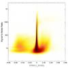 |
Fig. 5 Density plot of S/N vs. SExtractor’s SPREAD_MODEL for all detections. The dense vertical cloud located around SPREAD_MODEL is the point source (mostly stellar) locus. The fuzzy blob to the right of the stellar locus originates from galaxies and nebulosities, while the shallow cloud on the left is populated with cosmic ray hits and bad pixels. Note the asymmetry of the stellar locus caused by blended stars (most obvious at high S/N). |
7.5. Estimating astrometric uncertainties
Position uncertainties play a prominent role in our astrometric pipeline. They are the main ingredients of the relative weights given to individual detections in the global astrometric solution. They are also used as weights to compute robust proper motions and to identify outliers.
SExtractor’s 1-σ fitting-error ellipse parameters ERRAMODEL_IMAGE, ERRBMODEL_IMAGE and ERRTHETAMODEL_ IMAGE are directly extracted from the covariance matrix computed in the LevMar Levenberg-Marquardt minimization engine (Lourakis 2004). Based on repeatability tests performed on a wide range of simulated (photon-noise dominated) images, we checked that the estimated uncertainties matched the observed standard deviation of position residuals to better than 10% for isolated sources.
However, the dominant source of positional uncertainties for bright stars on ground-based exposures, with a duration of a few minutes or shorter, is not photon noise, but apparent relative motion caused by atmospheric turbulence. This motion is highly correlated at small angles (Schlesinger 1916); its impact on the estimation of proper motions is weak when working with very small fields of view, or when positions are measured relative to close neighbors. Neither is the case here, and the contribution from atmospheric turbulence component must be taken into account. In the regime probed by these observations (exposure time, field-of-view, telescope diameter), theoretical considerations as well as experimental studies (Lindegren 1980; Roddier 1981; Han 1989; Shao & Colavita 1992; Han & Gatewood 1995) have established that the amplitude of the relative random motion between two sources separated by angle θ (in arcmin) is well described by  (6)where T is the exposure time in seconds, and σ0m is the standard deviation expected in unit time for a pair of stars separated by ten arcmin.
Correlated “position noise” as described by Eq. (6) translates into non-diagonal terms in the measurement error matrix of detections from individual exposures. But since the current version of our astrometry solver ignores non-diagonal terms in the weighting matrix, we are left with considering only the variance averaged over individual fields. Part of this variance is “absorbed” in the deformable distortion model (Connes 1978; Lindegren 1980) such as the second-degree polynomial we are using (Sect. 7.6), but we assume this dampening effect to be weak considering the wide-fields of view of all the instruments involved here. The average contribution (per source) to pairwise positional variance due to relative motions in an exposure is half the integral of Eq. (6) over all possible pairs of positions within the FOV:  (7)For rectangular FOVs, we find that the following expression provides a good approximation (within 5% for aspect ratios <20:1) to σM(FOV):
 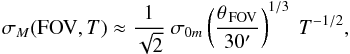 (8)where θ FOV is the diagonal of the field in arcmin.
Using star trails, Han & Gatewood (1995) measured σ0m = 54 mas at Mauna Kea, whereas Han (1989) reported a much higher σ0m = 143 mas at Allegheny observatory in Pittsburgh. Zacharias (1996), analyzing astrometric calibration residuals from short, repeated observations made at Kitt Peak and Cerro Tololo, found results compatible on average with Han & Gatewood’s value; although he claims that their exposures with best seeing exhibit a dispersion twice lower, and hints at a dependency of turbulence-induced motion with seeing. Our own measurements using short wide-field exposures from archive data (Bouy et al., in prep.), exhibit litte dependency on actual seeing and suggest that Han & Gatewood’s value is appropriate for observations carried out in good sites. We therefore add σM in quadrature to the measurement uncertainties estimated by SExtractor, adopting σ0m = 54 mas as well as the FOV and exposure time of the current image. Note that the current version of our astrometry engine assumes that position uncertainties are isotropic.
Another source of errors in the measurement of positions is imperfect deblending of close detections. Of particular concern for the astrometric solution are the detrimental effects of deblending errors in some bright sources. The impact of deblending on centroid measurements varies a lot from object to object and is difficult to quantify a priori. Nevertheless, we find that adding a 0.1 pixel error in quadrature to position uncertainties of detections flagged as “deblended” by SExtractor alleviates the problem with the bright sources, without downweighting excessively sources that have been properly deblended.
7.6. Computing a global astrometric solution
The global astrometric solution is computed with version 2.0 of the SCAMP software package (Bertin 2006). SCAMP is itself a mini-pipeline performing various operations before and after computing the global solution per se. These operations are described in detail in the SCAMP documentation; in the following we focus on those that are especially important for this study.
The global solution computed by SCAMP is the result of minimizing the quadratic sum of differences in position between overlapping detections from pairs of catalogs, an approach pioneered by Eichhorn (1960): 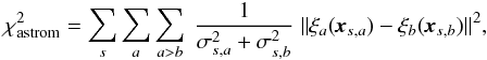 (9)where s is the source index, a and b are catalog indices, and σs,a is the positional uncertainty for source s in catalog a. For the purpose of computing a global solution, positions in Eq. (9) are in a common system of reprojected coordinates derived from raw detector coordinates x. For mosaic cameras, a catalog comprises several sub-catalogs for each exposure: one per detector chip. We express the reprojection operator ξc,e for chip c and exposure e as a combination of an undistorted reprojection operator
  derived from the (tangential) projection approximated at the initial cross-matching stage, and two polynomials describing instrumental distortions:
 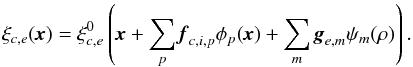 (10)The first polynomial with free coefficients fc,i,p describes static, chip-dependent (c) and instrument-dependent (i) distortions that are function of raw coordinates x. The second polynomial with free coefficients ge,m accounts for exposure-dependent distortions that are functions of focal-plane coordinates ρ, computed from the raw coordinates x using the initial positioning of chips on the focal plane. In this study we adopted a degree 4 for the chip-dependent polynomial, which in practice provides a very good fit to the geometrical distortions of most instruments. We chose a degree 2 for the exposure-dependent polynomial to account for flexures and geometric atmospheric refraction. Note that SCAMP automatically and progressively reduces the degree of both polynomials if the number of free parameters reaches or exceeds the number of constraints: detector failures, shallow exposures, etc.
The cameras involved in this study are often taken off the telescope between runs. Experience shows that the static part of the distortion pattern changes from run to run, sufficiently so to undermine the global solution. The same holfd for filter changes. Therefore the count of “astrometric instruments” entering Eq. (10) far exceeds that of cameras, because what matters eventually is the combination camera/filter/run. Relying on header information and logbooks, we identified 94 such combinations for the whole dataset, taken with 9 cameras through 30 filters.
For the minimum of  to be unique, the solution must be anchored on the sky. SCAMP does that by forcing one of the catalogs in Eq. (9) to be a catalog of astrometric references with fixed ξ coordinates. We selected 2MASS (Skrutskie et al. 2006) as a reference catalog because of its suitable depth, good homogeneity, and tight range of observation epochs.
Because instrumental distortions are weak at the scale of a chip (typically a few pixels), Eq. (10) can be well approximated by 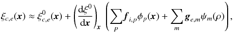 (11)which makes the minimization of Eq. (9) equivalent to solving a system of linear equations.
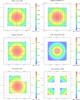 |
Fig. 6 Examples of camera distortion patterns, represented by maps of the pixel scale, for 6 of the 94 camera/filter/run combinations. |
In SCAMP, the astrometric solution is computed three times. A first distortion-free solution accurate to about 1′′ is obtained from the registration of all image exposures. This is sufficient to provide a satisfactory matching of most overlapping detections. A full global solution is then computed, which is used to identify detections with calibrated positions deviating excessively from the mean. Strong deviations may be caused by cross-matching problems such as blending or mismatches, differential chromatic refraction (at high airmass), wavelength-dependent centroids (in galaxies), or strong proper motions (in stars). Because of the extended range of epochs and the presence of a nearby star cluster in the data, we opted for a somewhat severe level of clipping, rejecting about 4.5% of all detections at this stage. The final run of the solver on this clipped sample yields the final set of distortion parameters. Figure 6 shows examples of recovered distortion patterns for some of the 94 camera/filter/run combinations.
SCAMP offers the possibility to produce maps of the average residuals in raw coordinates after calibrating the positions with the best-fitting distortion pattern models. These maps tell us of possible position-dependent systematic calibration errors, in particular distortion features that cannot be fitted with a fourth-degree polynomial. Two cameras appear to exhibit particularly striking residual patterns with most filter/runs (Fig. 7). A periodic, symmetric pattern is seen for NEWFIRM with amplitude ± 0.05 pixel, an indication that a fourth-degree polynomial is a poor fit to the distortion profile of this instrument. The WFCam data show coordinate jumps up to 0.08 pixel between rows 1024 and 1025 and between columns 1024 and 1025 columns. While the most obvious explanation for this feature would be small physical gaps between the four quadrants of the Hawaii-2 detectors (Cabelli et al. 2000), this “geometrical” hypothesis was dismissed by the Teledyne engineers we contacted, after a careful examination of the original mask used to manufacture the arrays. At the time of writing, we remain clueless about the origin of this matter, which is virtually undetectable using the UKIDSS data alone, because of the survey micro-dithering and tiling strategy.
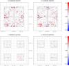 |
Fig. 7 x/y maps of systematic residuals (in pixels) for two camera/filter/run combinations. Top: NEWFIRM/J-band/Dec.-2009. Bottom: WFCam/Z-band/Dec.-2005. |
7.7. Differential chromatic refraction
Dispersive elements along the optical path (atmosphere, lenses) have wavelength-dependent refraction indices producing a color-dependent shift of the centroid (e.g., Filippenko 1982; Monet et al. 1992). This effect is known as differential chromatic refraction (DCR). The magnitude of atmospheric DCR depends on zenithal distance and on the source color index.
A prototype of empirical DCR correction is under development. It needs more testing, and has been turned off for the present study. Systematic errors due to DCR are nevertheless expected to be small:
-
The vast majority (95%) of the observations were obtained atairmass <1.4. The resulting absolute DCR offsets for B stars can add up to 30 mas in the V-band, 10 mas in the I-band and <1 mas in the H and K-bands under typical ambient conditions (Stone 2002). It goes down to 8, 7, 2 and ≪1 mas, respectively, for solar-type dwarfs, which corresponds to the high-mass end of our sensitivity limit, and rises again to ≈25 mas in V and 5 mas in I for late-M dwarfs. Relative offsets within the field-of-view of our instruments are expected to be even smaller.
-
The vast majority of the observations were obtained in the red or near-infrared part of the spectrum, where the amplitude of the DCR is smaller.
-
Several instruments used in this study are equipped with an atmospheric dispersion compensator (Subaru, CTIO/Mosaic2 and KPNO/Mosaic1)
-
Finally, for many sources, the effect of DCR on the proper motion fit is averaged over the large number of individual measurements (see Fig. 8).
7.8. Charge transfer inefficiency
Radiation damage of the CCD detectors can locally alter their charge tranfer efficiency (CTE), producing deformed PSFs and affecting the source extraction accuracy. While this effect is considerable in the space environment, it is expected to be negligible at the level of accuracy of our study in ground-based instruments. The complexity of the charge transfer inefficiency (CTI) effects and the large number of CCD instruments used in this study prevent us from attempting a systematic calibration. We nevertheless note that the dithering strategy used in the CCD observations is expected to average out the CTI effects on relative astrometry. Additionally, recent studies demonstrated that even a very low level of background strongly mitigates the CTI effects by filling the traps (Prod’homme et al. 2012). The sky background in ground-based CCD observations is several orders of magnitude higher than in space, and is expected to result in negligible CTI-induced distortion of stellar images. Finally, a large fraction of the observations was obtained with near-infrared detectors that are unaffected by CTI. We checked for a dependence of the residuals of the PSF fit and the astrometric solution on the S/N and distance to the amplifier, but found no systematic distorsion or offset following the behavior expected for CTI effects. For the remainder of the analysis, we consider the CTI effects to be negligible.
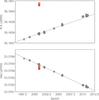 |
Fig. 8 Example of proper motion fit in right ascension (upper panel) and declination (lower panel). Red squares correspond to measurements rejected by the outlier filtering procedure. For most measurements the uncertainties are smaller than the symbol. A total of 93 individual exposures (out of 96 in total) were used for this source. See also Fig. 20. |
7.9. Computing proper motions
After the second iteration of the global astrometric calibration is completed, SCAMP performs another cross-matching of all detections, including those that were rejected at the previous step. SCAMP’s cross-matching algorithm matches in priority detections found in two or more successive exposures. We facilitate the cross-identification of moving sources by feeding SCAMP with exposures ordered by instrument and by observation date. We adopt a cross-matching radius of 3′′, which defines the maximum proper motion detectable in our study: ≈30′/h for the highest exposure rate found in our sample (one every 10 s).
SCAMP computes proper motions by performing a linear fit (in the weighted χ2 sense) to source positions as a function of observation dates. No attempt is made to include the effect of trigonometric parallaxes in the fit; annual parallaxes would be poorly constrained for most sources because of observation dates spanning a too short period of time each year. It is not unusual for the position of a source in a given exposure to deviate strongly from the linear trend with time expected from our model. Visual checks indicate that this happens most frequently because of a cosmetics problem (contamination by an electronic glitch, a cosmic ray hit, a fringing pattern, or an optical halo) or some deblending problem. To detect and filter out outliers, SCAMP applies a specific procedure to sources with more than two valid epochs and enduring a “poor” fit, i.e., with a reduced χ2 above 6. The procedure consists of removing from the fit the one detection that decreases the reduced χ2 the most, and iterate until it is lower than 6 or a maximum of 20% of points have been removed (or two points if fewer than ten points remain). With three detections, the the pair that corresponds to the lowest proper motion is selected. The filtering procedure is triggered on less than 5% of sources.
Figure 9 shows the distribution of the reduced χ2 as a function of magnitude and the number of measurements used in the proper motion fit. The reduced χ2s have values close to one over a large range of magnitude, a hint that the estimated measurements are robust and their uncertainties are reasonably well estimated.
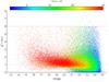 |
Fig. 9 Reduced χ2 of the proper motion fit as a function of the Megacam i-band magnitude (when available), with the number of measurements NPOS_OK indicated by color. The cut-off at χ2/d.o.f. = 6 corresponds to the outlier rejection threshold (see text). For clarity, only 10% of the catalog is represented. |
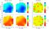 |
Fig. 10 Distribution of median proper motion of extragalactic sources in right ascension μαcosδ (upper panels) and declination μδ (lower panels). A gradient oriented towards the galactic plane is clearly visible. We adjust a fourth order polynomial surface (middle panels). The residuals of the fit are shown in the right panels. |
7.10. Anchoring to an absolute reference frame
The proper motions computed by SCAMP are not explicitly tied to an absolute reference system such as the International Celestial Reference System (ICRS). Our measurements can be linked to the ICRS by comparing them to the Hipparcos catalog. Unfortunately, most stars from the Hipparcos and Tycho catalogs present in the Pleiades field are saturated in our data. The resulting large uncertainties on the corresponding position and proper motion measurements prevent us from deriving an accurate offset to the ICRS. Nevertheless, we can tie our kinematic measurements very closely to the ICRS by computing the offset required to cancel out the apparent proper motion of extragalactic objects. The vast majority of galaxies detected in our sample are resolved under sub-arcsecond seeing conditions, and can therefore be easily and securely identified based on their SPREAD_MODEL value (Fig. 5). Even though the astrometric precision is considerably poorer for extended objects than for point sources, the large number of resolved extragalactic sources allows a statistically meaningful and accurate calculation of the offset to the ICRS. We selected all sources with a SPREAD_MODEL indicative of an extended object that display a proper motion weaker than 30 mas yr-1 in both RA and Dec (≈379 000 sources), and computed their median proper motion within boxes of 1° × 1°. Figure 10 shows the spatial distribution of median apparent proper motions μαcosδ and μδ. A gradient pointing toward the galactic plane is clearly seen in both components, which we interpret as the contribution of galactic stars to the overall astrometric solution derived by our algorithm. To correct for these systematic motions, we fit a fourth order polynomial surface to apparent motions in our “extragalactic” dataset and used it to correct all individual measurements. The residuals after correction are <0.2 mas yr-1, and we conservatively added 0.2 mas yr-1 quadratically to the final estimated uncertainty on the absolute proper motion.
As a sanity check, we then compared the proper motions of the 126 quasars from the Million Quasars (MILLIQUAS) Catalog (v.3.0) with a counterpart in our catalog. Figure 11 shows the vector point diagram obtained. As expected, the median proper motion is very close to zero (μαcosδ, μδ) = (0.29,0.17) mas yr-1.
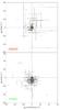 |
Fig. 11 Upper panel: vector point diagram for the 126 quasars from the Million Quasars Catalog with a counterpart in the DANCe catalog. Lower panel: vector point diagram for the 164 quasars with a counterpart in the PPMXL catalog. In both diagrams, the median value of the DANCe (red) and PPMXL (green) is represented by a large color dot. |
8. Photometric solution
A global photometric solution is computed for each photometric instrument. A photometric instrument is defined here as a set of instruments sharing a unique photometric behavior. In the case of our study, we chose to define one instrument per combination of telescope plus detector plus filter set. For example, although they are very similar (see Fig. 2), the CFH12K i-band photometric calibration was treated independently from that of the MegaCam i-band. This choice was made to minimize the effect of color terms between the various physical instruments. Similarly to astrometry, the photometric solution is computed through weighted χ2 minimization of the quadratic sum of magnitude differences between overlapping detections from pairs of exposures observed with the same photometric instrument. Color terms are ignored and the only free parameters are the magnitude zero-points. Wherever applicable, photometrically calibrated fields act as “anchors” in the final solution. No zero-point correction is applied to isolated fields. No attempt is currently made to derive illumination corrections for the various instruments: a uniform zero-point is computed for each exposure. Finally, the absolute zero-point calibration provided by the observatories or derived using standard fields obtained the same night is accurate to 0.01 to 0.05 mag for images obtained under clear or photometric conditions.
9. Limitations
9.1. Accuracy and sources of errors
The absolute astrometric accuracy is largely limited by the precision of the anchoring onto the extragalactic reference frame and is described in the previous section. The residuals add up to at most 0.2 mas yr-1 rms over the ≈10° of the survey. The overall “internal” (or relative, image-to-image) accuracy of the calibration is largely limited by the distorsion corrections residuals and the variable anisokinetism related to atmospheric turbulences. We also identify a number of sources of errors that can affect the proper motion measurements:
-
Cosmic rays and bad pixels can make chance coincidences andtherefore add noise to the astrometric solution. Theircontribution can be greatly minimized by i) using the mostup-to-date bad pixel masks for each instrument, ii) cleaningnon-overlapping images using Laplacian edge detection(van Dokkum 2001), iii) filteringabnormal measurements (in particular based on theSPREAD_MODEL of the sources, see Fig. 5), iv)rejecting outliers in the proper motion fit (seeSect. 7.9).
-
Artifacts produced by saturated stars (such as deformed PSFs, streaks, and bleeding due to pixel overflows) will seriously compromise the astrometric solution. This effect is minimized by carefully setting the saturation levels in SExtractor input parameter files. The SExtractor PSF fitting module is capable of adjusting a PSF to the non-saturated pixel of a source, which extends the dynamic range of our study above the saturation and non-linearity regime of the instruments used in this survey. The corresponding astrometry, although less precise, is nevertheless often good enough to derive relatively accurate proper motion, as illustrated in Fig. 13.
-
Extragalactic sources and nebulosities are often extended and their centroid position can be wavelength dependent. They can also surround point-like sources. The corresponding chromatic shift between overlapping images obtained in different filters can compromise the proper motion measurements, but also adds noise to the instrumental distortion measurement, and hence to the astrometric solution. The latter effect is minimized by carefully adjusting SExtractor’s parameters and by iteratively selecting only clean point-like sources for the astrometric registration, as described above. In particular, the SPREAD_MODEL filtering is expected to efficiently reject extended sources. Finally, these chromatic shifts are expected to be stochastic in orientation and amplitude, and their effect on the global solution should average out.
-
Unresolved multiple systems and visual binaries: the orbital motion of true multiple systems and the chromatic shift of blended pairs made of stars of different colors are an additional source of error that cannot be corrected for. Visual multiple systems resolved in a set of images and unresolved in another (e.g., when the seeing or sensitivity are different) can also produce mismatches and errors. They usually result in a high reduced-χ2 value.
-
Differential chromatic refraction errors, as discussed in Sect. 7.7.
-
Parallax motion: at an average distance of ≈120 pc (van Leeuwen 2009), the maximum amplitude of the parallax motion of Pleiades members is ≈8 mas yr-1. Our observations were obtained over yearly periods of approximately four months, and Pleiades members possibly display significant parallax motion. This effect is even stronger for nearby stars. Our observational strategy and the archival observations were not designed to measure parallaxes, and the multi-epoch images are not suited for a good parallax determination, which also adds noise to the astrometric solution and proper motion fit. We nevertheless verified that most of these sources (and in particular the Pleiades members) were rejected by the 1-σ clipping and their contribution to the astrometric solution is expected to be negligible.
-
Atmospheric turbulence, as discussed in Sect. 7.5. Using several consecutive observations allows one to additionally average this effect out, which also justifies using individual frames rather than stacked mosaics.
-
Proper motions themselves: although stars are clipped that strongly deviate because of proper motions, moderate motions (≈5−10 mas yr-1) may degrade the astrometric solution, which particularly affects the distortion patterns derived for the earliest and the latest runs in the observation time range. A new iterative procedure that recomputes the solution after correcting the positions of stars for the derived motions is under development in SCAMP, but it was not judged robust enough in its present state to be applied to this study.
Figure 12 shows the estimated error of the absolute proper motion fit4 as a function of the MegaCam i-band magnitude and the maximum time difference used for the fit. As expected, the estimated error is tightly correlated to the maximum time difference and to the luminosity.
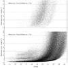 |
Fig. 12 Estimated error of the absolute proper motion measurements as a function of MegaCam i-band magnitude. Upper panel: for sources with a maximum time difference of less than 7 yr. Lower panel: for sources with a maximum time difference greater than 7 yr. |
10. Comparison with other astrometric catalogs
In the following, we compare our measurements with various astrometric databases found in the litterature and check the consistency of our results. Several of these catalogs are not tied to any absolute reference frame (e.g. UCAC4, UKIDSS), and a direct comparison with the DANCe catalog (anchored on background galaxies) is therefore not strictly correct. We nevertheless note that the difference can in general be approximated to a simple offset.
10.1. Tycho
The Tycho catalog (Høg et al. 2000) provides proper motion measurements precise to about 2.5 mas yr-1 and derived from a comparison of the ESA Hipparcos satellite measurements with the Astrographic Catalog and 143 other ground-based astrometric catalogs. These catalogs are unfortunately limited to VT ≲ 12.5 mag, very close to the saturation or non-linear regime of the datasets used to build the DANCe catalog. With this limitation in mind, we compare the results obtained for the 3665 common sources. The agreement is good within the large uncertainties, as shown in Fig. 13. As expected, the difference between the Tycho and DANCe measurement displays a clear dependance on the luminosity, fainter sources agreeing in general better than bright sources.
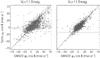 |
Fig. 13 Proper motion in RA for the DANCe (x-axis) and Tycho (y-axis) catalogs. The error bars represent the estimated error for the DANCe measurements and the reported uncertainty in the case of the Tycho measurement. The left panel corresponds to sources with VT < 11.5 mag, the right panel to sources with VT > 11.5 mag. A dashed line corresponding to a linear relation is represented to guide the eye. A similar distribution is found in declination. |
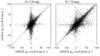 |
Fig. 14 Proper motion in RA for the DANCe (x-axis) and UCAC4 (y-axis) catalogs. Only a random subsample corresponding to 10% of the total number of matches is represented for clarity. The left panel corresponds to sources fainter than K = 13 mag, the right panel to sources brighter than K = 13 mag. A dashed line corresponding to a linear relation is represented to guide the eye. A similar distribution is found in declination. |
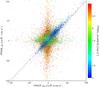 |
Fig. 15 Proper motion in RA for the DANCe (x-axis) and PPMXL (y-axis) catalogs.The color scale represents the PPMXL uncertainty. A similar distribution is found in declination. A dashed line corresponding to a linear relation is represented to guide the eye. |
10.2. UCAC4
The Fourth US Naval Observatory CCD Astrograph Catalog (UCAC4, Zacharias et al. 2010) provides astrometry, photometry, and proper motion measurements over the entire sky and covering the luminosity range between 8 ≲ R ≲ 16 mag. Uncertainties are typically of about 1–10 mas yr-1, depending on magnitude and observing history. Figure 14 shows a comparison of the proper motion measurements in RA for the UCAC4 and DANCe surveys as a function of 2MASS Ks-band luminosity. Three main groups of sources can be identified:
-
1.
“vertical outliers” are sources with close-to-zero motion inDANCe but significant motion in UCAC4;
-
2.
“horizontal outliers” are sources with close-to-zero motion in UCAC4 but significant motion in DANCe;
-
3.
sources with motions that agree well in both catalogs within the typical uncertainties and to a constant offset.
We found that both outlier groups are clearly related to the luminosity of the sources: the “vertical outliers” are in general among the faintest sources, where UCAC4 is less accurate and contains more errors. The “horizontal outliers” are in general bright sources, and we interpret them as erroneous or inaccurate measurements due to saturation and/or non-linearity of the DANCe datasets. As expected, the distribution of sources is asymmetric, with significantly more sources along the direction of the solar antapex (μαcosδ > 0 and μδ < 0), which coincidentally also corresponds to the Pleiades cluster’s mean motion direction.
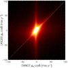 |
Fig. 16 Density map of the proper motion in RA for the DANCe (x-axis) and UKIDSS (y-axis) catalogs. A dashed line corresponding to a linear relation is represented to guide the eye. The same behaviour is found in declination. |
10.3. PPMXL
Roeser et al. (2010) derived improved mean positions and proper motions on the ICRS system by combining USNO-B1.0 and 2MASS astrometry. The catalog is complete from the brightest stars to about V ≈ 20 mag over the entire sky. Typical individual errors of the proper motions range between 4−10 mas yr-1. Figure 15 compares the proper motion measurements in RA and Dec for the PPMXL and DANCe surveys as a function of the PPMXL uncertainty. The same three groups of sources described in Sect. 10.2 can be seen:
-
1.
“vertical outliers” are sources with close-to-zero motion inDANCe but significant motion in PPMXL. They generally haveone or all of the following properties: a) they have the fewest Nonumber of measurements in PPXML, b) they are among thefaintest sources, and c) they have a flag fl = 1 in the PPMXL catalog indicative of a problematic fit. On the other hand, they seem to have a reasonable maximum time difference in the DANCe survey, which is in general associated with more reliable proper motion measurements;
-
2.
“horizontal outliers” with close-to-zero motion in PPMXL but significant motion in DANCe. These sources generally have the smallest maximum time difference and only a few individual measurements in the DANCe catalog, suggesting that the DANCe proper motion measurements are less reliable;
-
3.
sources with motions that agree well in both catalogs within the typical uncertainties.
We also note that in general the two outlier populations consist of the faintest sources, for which the astrometric precision is expected to be lower.
Figure 15 also shows an offset between the DANCe and PPMXL measurements, especially obvious in declination. Figure 11 suggests that the PPMXL proper motion measurements are indeed offset with respect to the ICRS, because quasars from the MILLIQUAS catalog have no average zero motion in the PPMXL catalog. A similar offset is also reported in the SPM4 catalog (see Fig. 8 of Girard et al. 2011).
10.4. UKIDSS DR9
The Pleiades cluster was observed as part of the UKIDSS Galactic Cluster Survey. Lodieu et al. (2012) recently presented a photometric and astrometric study based on the corresponding catalog, which includes proper motion measurements based on the multi-epoch UKIDSS observations. The proper motion measurements given in the UKIDSS DR9 catalog provide a useful comparison because the DANCe survey includes all the UKIDSS individual images. Figure 16 compares the proper motion measurements in RA for the UKIDSS and DANCe catalogs. Three main groups of sources appear clearly:
-
1.
“vertical outliers” are sources with close-to-zero motion inDANCe but significant motion in UKIDSS. In UKIDSS theygenerally have a) the fewest measurements (nFrames attribute);b) the highest star/galaxy classifier value, indicative of highprobability to be an extended extragalactic sources; and c) thelargest time difference in DANCe;
-
2.
sources with motions that agre well in both catalogs within the typical uncertainties and to a constant offset corresponding to the offset of the UKIDSS measurements to the ICRS;
-
3.
a diffuse group of sources that agree only poorly. Most of these sources are detected in the UKIDSS dataset only, and in general have a small maximum time difference resulting in larger uncertainties in the proper motion fit in both catalogs. The lose correlation and dispersion of this group are consistent with the typical uncertainties (>25 mas yr-1) of the corresponding measurements in both catalogs.
As the DANCe measurements for the vertical outliers correspond to the most probable extragalactic sources (which are supposed to have no detectable motion, in agreement with the DANCe measurements) and to the measurements with the longest DANCe time baseline (hence more robust in general), we are confident that the DANCe measurements of the vertical outliers are more reliable than their UKIDSS counterparts. We interpret the inconsistency for the vertical outliers’ population as a greater sensitivity of the UKIDSS proper motion fit to deviant individual astrometric measurements. The small number of measurements used in the proper motion fit (≤6) together with the lack of rejection in the UKIDSS proper motion fit (Lodieu et al. 2012) make it much more sensitive to deviant and high leverage points and translates into large numbers of errors. The corrupted frames in the UKIDSS DR9 release (discarded by our quality assurance but not by the UKIDSS quality assurance, M. Read priv. comm.) probably also result in a number of problematic measurements. By using the individual UKIDSS images rather than stacked UKIDSS mosaics, and by including a robust regression algorithm for the proper motion fit, our method is much less sensitive to erroneous individual measurements, as demonstrated by the lack of a clear “horizontal outliers” population.
10.5. Using the DANCe and other astrometric catalogs
Large catalogs necessarily contain errors and problems. The comparison of the DANCe measurements with other astrometric catalogs calls for a number of important warnings about their use:
-
some proper motion measurements are more reliable than others,and the uncertainty does not always reflect the reliability.Parameters useful to evaluate the reliability of an individualproper motion measurement include in particular (but notexhaustively) the number of astrometric measurements used forthe fit, the maximum time baseline, the reduced-χ2 of the fit
-
measurements errors, unknown systematics and problematic measurements present in any large scale astrometric catalog most likely always affect the completeness of studies based on their proper motion measurements and should be carefully discussed.
While a universal rule to assess the quality of a given measurement cannot be given, we have found that the following proper motion measurements should be considered with caution:
-
sources close to or above the saturation or linearity limit of theinstruments (in the case of the current dataset, i ≈ 13 mag); or
-
sources with small numbers of measurements used for the proper motion fit (NPOS_OK attribute);
-
sources with large reduced-χ2 (CHI2_ASTROM attribute).
In general, and whenever possible, a visual inspection of the individual images is the most reliable way to discard problematic measurements.
11. Example of scientific applications
The DANCe catalog includes accurate photometry and astrometry for 6 116 907 unique sources and proper motion measurements for 3 577 478 of them, and as such represents a unique opportunity to address various scientific problems. In the following, we give a few examples of direct applications of the catalog.
11.1. The Pleiades cluster
A detailed scientific analysis of the Pleiades cluster kinematics based on the DANCe catalog will be presented in a future article (Bouy et al., in prep.). In this section, we give a brief and general overview of the results obtained. Figure 17 shows the vector point diagram of stellar motions obtained with the dataset described above. The group of co-moving cluster members appears clearly around (20,−40) mas yr-1.
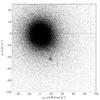 |
Fig. 17 Vector point diagram of stellar motions obtained with the datasets described in this article. The Pleiades locus is visible in the lower right quadrant. Its slight elongation may be interpreted as a perspective effect related to the depth of the cluster. |
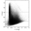 |
Fig. 18 i vs. r − i color magnitude diagram (MegaCam). Two horizontal lines represent the luminosity of Pleiades members with masses 0.072 and 0.030 M⊙, according to the models of Baraffe et al. (1998) and assuming of distance of 120 pc. The Pleiades sequence is visible. |
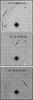 |
Fig. 19 Successive CFHT MegaCam images of a main belt asteroid of g = 23.1 mag. The UT time of observations are indicated. These three images are an illustrative subset of 19 images used to measure the proper motion of this source. |
The DANCe catalog also offers a unique photometric database. For the Pleiades dataset presented here, a total of 29 photometric instruments covering the spectral range between 0.37 μm (Sloan u-band) and 2.2 μm (UKIRT K-band). Figure 18 shows a i vs. r − i color magnitude diagram using the photometry extracted from the MegaCam and UKIDSS images. The cluster sequence is also visible.
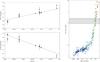 |
Fig. 20 Relative motion in RA (upper left panel) and Dec (lower left panel) of a candidate T5 dwarf discovered in the survey. WISE [W1]−[W2] colors of ultracool dwarfs from Kirkpatrick et al. (2011). The color of our new candidate is indicated with a horizontal line, and the uncertainty domain is represented by a light-gray area. |
11.2. Solar-system bodies
Solar-system bodies have typical velocities in the range between ≈2′′ h-1 (trans-Neptunian objects, hereafter TNO) and ≈20′′ h-1 (main belt asteroids, hereafter MBA). Most observations used in this study consist of several consecutive and dithered images of the same field. Fast-moving sources such as solar-system bodies can therefore be easily identified. Minor planets are expected to be extremely numerous in the direction of the Pleiades cluster, because it lies close to the ecliptic plane. A detailed analysis of the solar-system bodies encountered in the DANCe dataset will be presented in a future article (Bouy et al. in prep) and we only give a brief overview of the capabilities of our algorithms for solar-system studies. A basic selection of all sources with a proper motion greater than ≈20′′ h-1 yielded 11404 candidate minor planets. A request on SkyBot (Berthier et al. 2006) indicates that only 2837 have a counterpart within a radius of 1′ in the database of known solar-system bodies as of August 2012, all of them main belt asteroids. A visual inspection of ≈100 random candidates shows that ≲5% are false detections due to artifacts (cosmic ray or ghost coincidence, false detection, etc). After inspection and rejection of these artifacts, the astrometric and photometric measurements will be submitted to the IAU Minor Planet Center. The high-precision astrometry (with a typical accuracy better than ≲10 mas on individual epochs) will be extremely valuable to refine the orbital solutions. The accurate photometry (with typical absolute accuracy <10% and relative accuracy better than ≪1%) will be useful for classifying the bodies (based on their colors) and in some cases studying their rotational periods and geometry. The depth of the datasets allows the discovery of very faint objects, as illustrated in Fig. 19, probing a largely incomplete asteroid size domain.
11.3. Nearby ultracool dwarfs
Nearby ultracool dwarfs can easily be identified in the DANCe catalogs as faint fast-moving sources. Figure 20 shows an example of such an object discovered in the present survey. A complete analysis will be presented in a future paper, and we here only present the basic properties of one particular source to illustrate the scientific case. The source must be relatively nearby because it moves at ≈200 mas yr-1. It has a counterpart in the WISE (Cutri et al. 2012) and its [W1]−[W2] color matches that of known T4 ~ T5 ultracool dwarfs from Kirkpatrick et al. (2011).
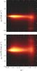 |
Fig. 21 Density maps showing the distribution of proper motion in RA (upper panel) and Dec (lower panel) as a function of the g − r color for galactic sources in the range 12 < g < 21 mag. |
11.4. Galactic dynamics
Accurate large-scale photometric and astrometric surveys provide a unique opportunity for studying the galactic stellar populations. In Fig. 21, we show the distribution of motions in RA and Dec as a function of the g − r color. For this figure, a subset of galactic sources was selected in the DANCe catalog based on
-
the quality of the proper motion measurement, keeping sourceswith g magnitude in the range 12–21 mag where the estimated uncertainties are better than ≲2 mas yr-1 on average.
-
the “stellarity”, rejecting all sources with a SPREAD_MODEL indicative of an extended source. Although it does not reject unresolved extragalactic sources, the remaining extragalactic contamination on the luminosity range mentioned above should be weak enough for the simple purpose of this illustrative example
A gross bimodal structure in g − r is clearly seen, reflecting the separation of the halo/thick-disk (g − r ~ 0.5 mag) and the thin-disk (g − r ~ 1.3 mag) populations. The Pleiades population is clearly seen as a small clump around (20, −40) mas yr-1 on top of the general thin disk population. Such observations can provide very important constraints and input for models of galactic populations.
12. Conclusions and prospects
We have presented a set of tools capable of deriving high-precision relative proper motions using large numbers (several thousands) of ground-based images originating from various instruments. We applied these tools to multi-epoch panchromatic datasets of the nearby Pleiades cluster, and compared our results to other astrometric catalogs. The results demonstrate our ability to derive proper motions with an estimated accuracy better than 1 mas yr-1 for sources as faint as i = 22 ~ 23 mag, depending on the luminosity and observational history (time baseline, number and quality of the frames, as well as presence and number of reference extragalactic sources for the anchoring on the ICRS).
The DANCe project will use this method to conduct a survey of the most nearby star-forming regions and clusters. It aims at complementing the Gaia mission in the substellar regime and in regions of high extinction. By taking advantage of the wide-field surveys performed in the late 90s and early 2000s, it will provide high-precision proper motion measurements for millions of stars in various nearby associations. In the future, the DANCe project will also take advantage of the growing number of wide and very wide-field imagers that will equip various observatories. Large and all-sky surveys are also ongoing (e.g. Pann-STARRS,ESO-VST, ESO-VISTA) or foreseen (DES, LSST), ensuring a huge flow of high-quality images useable for high-precision astrometry.
The transmission curves were retrieved from the Spanish VO website http://svo2.cab.inta-csic.es/theory/fps/
IRAF is distributed by the National Optical Astronomy Observatory, which is operated by the Association of Universities for Research in Astronomy (AURA) under cooperative agreement with the National Science Foundation.
Computed as the quadratic sum of the RA and Dec components, and the 0.2 mas yr-1 residual related to the anchoring onto the ICRS.
Acknowledgments
We are thankful to our anonymous referee for a thorough and constructive review that helped to significantly improve this article. H. Bouy is funded by the the Ramón y Cajal fellowship program number RYC-2009-04497. H. Bouy acknowledges funding and support of the Université Joseph Fourier 1, Grenoble, France. This research has been funded by Spanish grants AYA2012-38897-C02-01, AYA2010-21161-C02-02, CDS2006-00070 and PRICIT-S2009/ESP-1496. E. Moraux ackowledges funding from the Agence Nationale pour la Recherche program ANR 2010 JCJC 0501 1 “DESC (Dynamical Evolution of Stellar Clusters)”. J. Bouvier acknowledges funding form the Agence Nationale pour la Recherche program ANR 2011 Blanc SIMI 5-6 020 01 (“Toupies”). J. Bouvier and E. Moraux acknowledge support from the Faculty of the European Space Astronomy Centre (ESAC). A. Bayo ackowledges funding and support from the Marie Curie Actions of the European Commission FP7-COFUND. E. Bertin acknowledges partial funding of computer resources by the French Programme National de Cosmologie et Galaxies and CNRS-Fermilab contract #367561. We are grateful to Mike Read and Mike Irwin for their help and assistance with the INT and UKIRT archives, and to Mark Farris and James Beletic at Teledyne for looking into the pixel grid issue with the WFCam Hawaii-2 detectors.
Based on observations obtained with MegaPrime/MegaCam, a joint project of CFHT and CEA/DAPNIA, at the Canada-France-Hawaii Telescope (CFHT) which is operated by the National Research Council (NRC) of Canada, the Institut National des Science de l’Univers of the Centre National de la Recherche Scientifique (CNRS) of France, and the University of Hawaii. This paper makes use of data obtained from the Isaac Newton Group Archive, which is maintained as part of the CASU Astronomical Data Centre at the Institute of Astronomy, Cambridge. The data were made publically available through the Isaac Newton Group’s Wide-Field Camera Survey Programme. The Isaac Newton Telescope is operated on the island of La Palma by the Isaac Newton Group in the Spanish Observatorio del Roque de los Muchachos of the Instituto de Astrofísica de Canarias. This research used the facilities of the Canadian Astronomy Data Centre operated by the National Research Council of Canada with the support of the Canadian Space Agency. This research draws upon data provided by C. Briceño as distributed by the NOAO Science Archive. NOAO is operated by the Association of Universities for Research in Astronomy (AURA) under cooperative agreement with the National Science Foundation. This publication makes use of data products from the Two Micron All Sky Survey, which is a joint project of the University of Massachusetts and the Infrared Processing and Analysis Center/California Institute of Technology, funded by the National Aeronautics and Space Administration and the National Science Foundation. This work is based in part on data obtained as part of the UKIRT Infrared Deep Sky Survey. This research has made use of the VizieR and Aladin images and catalog access tools and of the SIMBAD database, operated at CDS, Strasbourg, France. This research has made use of IMCCE’s SkyBoT VO tool. This publication makes use of data products from the Wide-field Infrared Survey Explorer, which is a joint project of the University of California, Los Angeles, and the Jet Propulsion Laboratory/California Institute of Technology, funded by the National Aeronautics and Space Administration. This research has made use of the Million Quasars (MILLIQUAS) Catalog, Version 3.0 (9 September 2012). The MILLIQUAS Catalog made use of NASA/IPAC Extragalactic Database (NED) which is operated by the Jet Propulsion Laboratory, California Institute of Technology, under contract with the National Aeronautics and Space Administration, and also made use of data obtained from the Chandra Source Catalog, provided by the Chandra X-ray Center (CXC) as part of the Chandra Data Archive.
References
- Adams, F. C. 2001, in From Darkness to Light: Origin and Evolution of Young Stellar Clusters, eds. T. Montmerle, & P. André, ASP Conf. Ser., 243, 291 [Google Scholar]
- Anderson, J., Bedin, L. R., Piotto, G., Yadav, R. S., & Bellini, A. 2006, A&A, 454, 1029 [NASA ADS] [CrossRef] [EDP Sciences] [Google Scholar]
- Autry, R. G., Probst, R. G., Starr, B. M., et al. 2003, in SPIE Conf. Ser. 4841, eds. M. Iye, & A. F. M. Moorwood, 525 [Google Scholar]
- Baraffe, I., Chabrier, G., Allard, F., & Hauschildt, P. H. 1998, A&A, 337, 403 [NASA ADS] [Google Scholar]
- Baraffe, I., Chabrier, G., & Gallardo, J. 2009, ApJ, 702, L27 [NASA ADS] [CrossRef] [Google Scholar]
- Barrado y Navascués, D., Stauffer, J. R., Bouvier, J., Jayawardhana, R., & Cuillandre, J.-C. 2004, ApJ, 610, 1064 [NASA ADS] [CrossRef] [Google Scholar]
- Bayo, A., Barrado, D., Stauffer, J., et al. 2011, A&A, 536, A63 [NASA ADS] [CrossRef] [EDP Sciences] [Google Scholar]
- Béjar, V. J. S., Martín, E. L., Zapatero Osorio, M. R., et al. 2001, ApJ, 556, 830 [NASA ADS] [CrossRef] [Google Scholar]
- Bellini, A., & Bedin, L. R. 2010, A&A, 517, A34 [NASA ADS] [CrossRef] [EDP Sciences] [Google Scholar]
- Bellini, A., Piotto, G., Bedin, L. R., et al. 2009, A&A, 493, 959 [NASA ADS] [CrossRef] [EDP Sciences] [Google Scholar]
- Berthier, J., Vachier, F., Thuillot, W., et al. 2006, in Astronomical Data Analysis Software and Systems XV, eds. C. Gabriel, C. Arviset, D. Ponz, & S. Enrique, ASP Conf. Ser., 351, 367 [Google Scholar]
- Bertin, E. 2006, in Astronomical Data Analysis Software and Systems XV, eds. C. Gabriel, C. Arviset, D. Ponz, & S. Enrique, ASP Conf. Ser., 351, 112 [Google Scholar]
- Bertin, E. 2010, in JENAM 2010, Joint European and National Astronomy Meeting [Google Scholar]
- Bertin, E. 2011, in Astronomical Data Analysis Software and Systems XX, eds. I. N. Evans, A. Accomazzi, D. J. Mink, & A. H. Rots, ASP Conf. Ser., 442, 435 [Google Scholar]
- Bertin, E., & Arnouts, S. 1996, A&AS, 117, 393 [NASA ADS] [CrossRef] [EDP Sciences] [Google Scholar]
- Bobylev, V. V. 2006, Astron. Lett., 32, 816 [NASA ADS] [CrossRef] [Google Scholar]
- Boulade, O., Charlot, X., Abbon, P., et al. 2003, in SPIE Conf. Ser. 4841, eds. M. Iye, & A. F. M. Moorwood, 72 [Google Scholar]
- Bouvier, J., Stauffer, J. R., Martín, E. L., et al. 1998, A&A, 336, 490 [NASA ADS] [Google Scholar]
- Bouy, H., Bertin, E., Cuillandre, J. C., et al. 2011, in Stellar Clusters and Associations: A RIA Workshop on Gaia, 103 [Google Scholar]
- Brandner, W., Alcala, J. M., Kunkel, M., Moneti, A., & Zinnecker, H. 1996, A&A, 307, 121 [NASA ADS] [Google Scholar]
- Cabelli, C. A., Cooper, D. E., Haas, A. K., et al. 2000, SPIE Conf. Ser. 4028, eds. E. L. Dereniak, & R. E. Sampson, 331 [Google Scholar]
- Casali, M., Adamson, A., Alves de Oliveira, C., et al. 2007, A&A, 467, 777 [NASA ADS] [CrossRef] [EDP Sciences] [Google Scholar]
- Connes, P. 1978, in IAU Colloq. 48: Mod. Astrometry, eds. F. V. Prochazka, & R. H. Tucker, 339 [Google Scholar]
- Cuillandre, J.-C., Luppino, G. A., Starr, B. M., & Isani, S. 2000, in SPIE Conf. Ser., eds. M. Iye, & A. F. Moorwood, 1010 [Google Scholar]
- Cuillandre, J.-C., Magnier, E. A., Isani, S., et al. 2004, in Scientific Detectors for Astronomy, The Beginning of a New Era, eds. P. Amico, J. W. Beletic, & J. E. Belectic, 287 [Google Scholar]
- Cutri, R. M., et al. 2012, VizieR Online Data Catalog II/311 [Google Scholar]
- Desai, S., Armstrong, R., Mohr, J. J., et al. 2012, ApJ, 757, 83 [NASA ADS] [CrossRef] [Google Scholar]
- Dobbie, P. D., Kenyon, F., Jameson, R. F., et al. 2002, MNRAS, 335, 687 [NASA ADS] [CrossRef] [Google Scholar]
- Duchon, C. E. 1979, J. Appl. Meteorol., 18, 1016 [NASA ADS] [CrossRef] [Google Scholar]
- Eichhorn, H. 1960, Astron. Nachr., 285, 233 [Google Scholar]
- Eiroa, C., & Casali, M. M. 1992, A&A, 262, 468 [NASA ADS] [Google Scholar]
- Filippenko, A. V. 1982, PASP, 94, 715 [NASA ADS] [CrossRef] [Google Scholar]
- Gálvez-Ortiz, M. C., Clarke, J. R. A., Pinfield, D. J., et al. 2010, MNRAS, 409, 552 [NASA ADS] [CrossRef] [Google Scholar]
- Gilmore, G., Randich, S., Asplund, M., et al. 2012, The Messenger, 147, 25 [NASA ADS] [Google Scholar]
- Girard, T. M., van Altena, W. F., Zacharias, N., et al. 2011, AJ, 142, 15 [NASA ADS] [CrossRef] [Google Scholar]
- Hambly, N. C., Collins, R. S., Cross, N. J. G., et al. 2008, MNRAS, 384, 637 [NASA ADS] [CrossRef] [Google Scholar]
- Han, I. 1989, AJ, 97, 607 [NASA ADS] [CrossRef] [Google Scholar]
- Han, I., & Gatewood, G. D. 1995, PASP, 107, 399 [NASA ADS] [CrossRef] [Google Scholar]
- Høg, E., Fabricius, C., Makarov, V. V., et al. 2000, A&A, 355, L27 [NASA ADS] [Google Scholar]
- Ives, D. 1998, IEEE Spectrum, 16, 20 [NASA ADS] [Google Scholar]
- Ivezić, Ž., Lupton, R. H., Schlegel, D., et al. 2004, Astron. Nachr., 325, 583 [NASA ADS] [CrossRef] [Google Scholar]
- Jeffries, R. D., Maxted, P. F. L., Oliveira, J. M., & Naylor, T. 2006, MNRAS, 371, L6 [NASA ADS] [CrossRef] [Google Scholar]
- Kharchenko, N. V., Piskunov, A. E., Röser, S., Schilbach, E., & Scholz, R. 2005, A&A, 438, 1163 [NASA ADS] [CrossRef] [EDP Sciences] [MathSciNet] [Google Scholar]
- King, I. R. 1983, PASP, 95, 163 [NASA ADS] [CrossRef] [Google Scholar]
- Kirkpatrick, J. D., Cushing, M. C., Gelino, C. R., et al. 2011, ApJS, 197, 19 [NASA ADS] [CrossRef] [Google Scholar]
- Knödlseder, J. 2000, A&A, 360, 539 [NASA ADS] [Google Scholar]
- Köhler, R., Kunkel, M., Leinert, C., & Zinnecker, H. 2000, A&A, 356, 541 [NASA ADS] [Google Scholar]
- Kraus, A. L., & Hillenbrand, L. A. 2007, ApJ, 662, 413 [NASA ADS] [CrossRef] [Google Scholar]
- Landolt, A. U. 1992, AJ, 104, 340 [NASA ADS] [CrossRef] [Google Scholar]
- Lawrence, A., Warren, S. J., Almaini, O., et al. 2007, MNRAS, 379, 1599 [NASA ADS] [CrossRef] [MathSciNet] [Google Scholar]
- Lindegren, L. 1980, A&A, 89, 41 [Google Scholar]
- Lodieu, N., Bouvier, J., James, D. J., et al. 2006, A&A, 450, 147 [NASA ADS] [CrossRef] [EDP Sciences] [Google Scholar]
- Lodieu, N., Dobbie, P. D., Deacon, N. R., et al. 2007a, MNRAS, 380, 712 [NASA ADS] [CrossRef] [Google Scholar]
- Lodieu, N., Hambly, N. C., Jameson, R. F., et al. 2007b, MNRAS, 374, 372 [NASA ADS] [CrossRef] [Google Scholar]
- Lodieu, N., Deacon, N. R., & Hambly, N. C. 2012, MNRAS, 422, 1495 [NASA ADS] [CrossRef] [Google Scholar]
- López Martí, B., Jiménez-Esteban, F., & Solano, E. 2011, A&A, 529, A108 [NASA ADS] [CrossRef] [EDP Sciences] [Google Scholar]
- Lourakis, M. 2004, levmar: Levenberg-Marquardt nonlinear least squares algorithms in C/C++, http:// [0]www. [0]ics. [0]forth. [0]gr/ [0]~lourakis/ [0]levmar/ [Google Scholar]
- Magnier, E. A., & Cuillandre, J.-C. 2004, PASP, 116, 449 [NASA ADS] [CrossRef] [Google Scholar]
- Mahadevan, S., Ge, J., van Eyken, J., et al. 2007, in BAAS AAS/Division for Planetary Sciences Meeting Abstracts, 39, 466 [Google Scholar]
- Majewski, S. R., Skrutskie, M. F., Schiavon, R. P., et al. 2007, in BAAS, Am. Astron. Soc. Meet. Abstracts, 39, 132.08 [Google Scholar]
- Malapert, J.-C., & Magnard, F. 2006, in Astronomical Data Analysis Software and Systems XV, eds. C. Gabriel, C. Arviset, D. Ponz, & S. Enrique, ASP Conf. Ser., 351, 731 [Google Scholar]
- Marks, M., & Kroupa, P. 2012, A&A, 543, A8 [NASA ADS] [CrossRef] [EDP Sciences] [Google Scholar]
- Mathieu, R. D. 2000, in Stellar Clusters and Associations: Convection, Rotation, and Dynamos, eds. R. Pallavicini, G. Micela, & S. Sciortino, ASP Conf. Ser., 198, 517 [Google Scholar]
- McFarland, J. P., Helmich, E. M., & Valentijn, E. A. 2012, Exp. Astron., 19 [Google Scholar]
- McMahon, R. G., Walton, N. A., Irwin, M. J., et al. 2001, New Astron. Rev., 45, 97 [NASA ADS] [CrossRef] [Google Scholar]
- Metzger, M. R., Luppino, G. A., & Miyazaki, S. 1995, in BAAS, 27, 1389 [Google Scholar]
- Miyazaki, S., Komiyama, Y., Sekiguchi, M., et al. 2002, PASJ, 54, 833 [NASA ADS] [CrossRef] [Google Scholar]
- Mohr, J. J., Armstrong, R., Bertin, E., et al. 2012, Software and Cyberinfrastructure for Astronomy II, Proc. SPIE, 8451, id. 84510D [Google Scholar]
- Monet, D. G., Dahn, C. C., Vrba, F. J., et al. 1992, AJ, 103, 638 [NASA ADS] [CrossRef] [Google Scholar]
- Moraux, E., Bouvier, J., & Stauffer, J. R. 2001, A&A, 367, 211 [NASA ADS] [CrossRef] [EDP Sciences] [Google Scholar]
- Moraux, E., Bouvier, J., Stauffer, J. R., & Cuillandre, J.-C. 2003, A&A, 400, 891 [NASA ADS] [CrossRef] [EDP Sciences] [Google Scholar]
- Ouchi, M., Shimasaku, K., Okamura, S., et al. 2004, ApJ, 611, 660 [NASA ADS] [CrossRef] [Google Scholar]
- Perryman, M. A. C., Lindegren, L., Kovalevsky, J., et al. 1997, A&A, 323, L49 [NASA ADS] [Google Scholar]
- Perryman, M. A. C., de Boer, K. S., Gilmore, G., et al. 2001, A&A, 369, 339 [NASA ADS] [CrossRef] [EDP Sciences] [Google Scholar]
- Prod’homme, T., Holl, B., Lindegren, L., & Brown, A. G. A. 2012, MNRAS, 419, 2995 [NASA ADS] [CrossRef] [Google Scholar]
- Proszkow, E., & Adams, F. C. 2009, ApJS, 185, 486 [NASA ADS] [CrossRef] [Google Scholar]
- Roddier, F. 1981, Progress in optics 19 (Amsterdam, North-Holland Publishing Co), 19, 281 [Google Scholar]
- Roeser, S., Demleitner, M., & Schilbach, E. 2010, AJ, 139, 2440 [NASA ADS] [CrossRef] [Google Scholar]
- Schlesinger, F. 1916, Publications of the Allegheny Observatory of the University of Pittsburgh, 3, 1 [NASA ADS] [Google Scholar]
- Shao, M., & Colavita, M. M. 1992, A&A, 262, 353 [NASA ADS] [Google Scholar]
- Skrutskie, M. F., Cutri, R. M., Stiening, R., et al. 2006, AJ, 131, 1163 [NASA ADS] [CrossRef] [Google Scholar]
- Stauffer, J. R., Hartmann, L. W., Fazio, G. G., et al. 2007, ApJS, 172, 663 [NASA ADS] [CrossRef] [Google Scholar]
- Steinmetz, M., Zwitter, T., Siebert, A., et al. 2006, AJ, 132, 1645 [NASA ADS] [CrossRef] [Google Scholar]
- Stone, R. C. 2002, PASP, 114, 1070 [NASA ADS] [CrossRef] [Google Scholar]
- Swaters, R. A., Valdes, F., & Dickinson, M. E. 2009, in Astronomical Data Analysis Software and Systems XVIII, eds. D. A. Bohlender, D. Durand, & P. Dowler, ASP Conf. Ser., 411, 506 [Google Scholar]
- Torres, C. A. O., Quast, G. R., da Silva, L., et al. 2006, A&A, 460, 695 [NASA ADS] [CrossRef] [EDP Sciences] [Google Scholar]
- Torres, C. A. O., Quast, G. R., Melo, C. H. F., & Sterzik, M. F. 2008, in Handbook of Star Forming Regions, ed. B. Reipurth, (ASP), 757 [Google Scholar]
- van Dokkum, P. G. 2001, PASP, 113, 1420 [NASA ADS] [CrossRef] [Google Scholar]
- van Leeuwen, F. 2009, A&A, 497, 209 [NASA ADS] [CrossRef] [EDP Sciences] [Google Scholar]
- Wolfe, T., Armandroff, T., Blouke, M. M., et al. 2000, in SPIE Conf. Ser. 3965, eds. M. M. Blouke, N. Sampat, G. M. Williams, & T. Yeh, 80 [Google Scholar]
- Yadav, R. K. S., Bedin, L. R., Piotto, G., et al. 2008, A&A, 484, 609 [NASA ADS] [CrossRef] [EDP Sciences] [Google Scholar]
- Yagi, M., Kashikawa, N., Sekiguchi, M., et al. 2002, AJ, 123, 66 [NASA ADS] [CrossRef] [Google Scholar]
- Zacharias, N. 1996, PASP, 108, 1135 [NASA ADS] [CrossRef] [Google Scholar]
- Zacharias, N., Finch, C., Girard, T., et al. 2010, AJ, 139, 2184 [NASA ADS] [CrossRef] [Google Scholar]
- Zapatero Osorio, M. R., Rebolo, R., Martín, E. L., et al. 1999, A&AS, 134, 537 [NASA ADS] [CrossRef] [EDP Sciences] [Google Scholar]
- Zuckerman, B., Webb, R. A., Schwartz, M., & Becklin, E. E. 2001, ApJ, 549, L233 [NASA ADS] [CrossRef] [Google Scholar]
- Zuckerman, B., Song, I., & Bessell, M. S. 2004, ApJ, 613, L65 [NASA ADS] [CrossRef] [Google Scholar]
- Zuckerman, B., Bessell, M. S., Song, I., & Kim, S. 2006, ApJ, 649, L115 [NASA ADS] [CrossRef] [Google Scholar]
All Tables
All Figures
|
Fig. 1 IRAS 100 μm image of the Pleiades cluster with the various surveys used in this study overplotted. The Seven Sisters are represented with yellow stars. The full Moon is represented in the lower right corner to illustrate the scale. |
| In the text | |
|
Fig. 2 Transmission of the various filters used in this study. In the z-band, the sensitivity is limited by the CCD quantum efficiency, which typically drops at 900 ~ 1000 nm. |
| In the text | |
|
Fig. 3 Upper panel: distribution of airmass for the observations. Lower panel: distribution of FWHM of all the individual unresolved detections. The lines represents the cumulative distribution. |
| In the text | |
|
Fig. 4 Example of PSF reconstruction on one of the exposures (NEWFIRM frame K4N09B_20091221-0011K-kp). Left: snapshots of the variable PSF model over the field of view. Center: distribution of the PSF model FWHM. Right: distribution of the PSF model ellipticity. |
| In the text | |
|
Fig. 5 Density plot of S/N vs. SExtractor’s SPREAD_MODEL for all detections. The dense vertical cloud located around SPREAD_MODEL is the point source (mostly stellar) locus. The fuzzy blob to the right of the stellar locus originates from galaxies and nebulosities, while the shallow cloud on the left is populated with cosmic ray hits and bad pixels. Note the asymmetry of the stellar locus caused by blended stars (most obvious at high S/N). |
| In the text | |
|
Fig. 6 Examples of camera distortion patterns, represented by maps of the pixel scale, for 6 of the 94 camera/filter/run combinations. |
| In the text | |
|
Fig. 7 x/y maps of systematic residuals (in pixels) for two camera/filter/run combinations. Top: NEWFIRM/J-band/Dec.-2009. Bottom: WFCam/Z-band/Dec.-2005. |
| In the text | |
|
Fig. 8 Example of proper motion fit in right ascension (upper panel) and declination (lower panel). Red squares correspond to measurements rejected by the outlier filtering procedure. For most measurements the uncertainties are smaller than the symbol. A total of 93 individual exposures (out of 96 in total) were used for this source. See also Fig. 20. |
| In the text | |
|
Fig. 9 Reduced χ2 of the proper motion fit as a function of the Megacam i-band magnitude (when available), with the number of measurements NPOS_OK indicated by color. The cut-off at χ2/d.o.f. = 6 corresponds to the outlier rejection threshold (see text). For clarity, only 10% of the catalog is represented. |
| In the text | |
|
Fig. 10 Distribution of median proper motion of extragalactic sources in right ascension μαcosδ (upper panels) and declination μδ (lower panels). A gradient oriented towards the galactic plane is clearly visible. We adjust a fourth order polynomial surface (middle panels). The residuals of the fit are shown in the right panels. |
| In the text | |
|
Fig. 11 Upper panel: vector point diagram for the 126 quasars from the Million Quasars Catalog with a counterpart in the DANCe catalog. Lower panel: vector point diagram for the 164 quasars with a counterpart in the PPMXL catalog. In both diagrams, the median value of the DANCe (red) and PPMXL (green) is represented by a large color dot. |
| In the text | |
|
Fig. 12 Estimated error of the absolute proper motion measurements as a function of MegaCam i-band magnitude. Upper panel: for sources with a maximum time difference of less than 7 yr. Lower panel: for sources with a maximum time difference greater than 7 yr. |
| In the text | |
|
Fig. 13 Proper motion in RA for the DANCe (x-axis) and Tycho (y-axis) catalogs. The error bars represent the estimated error for the DANCe measurements and the reported uncertainty in the case of the Tycho measurement. The left panel corresponds to sources with VT < 11.5 mag, the right panel to sources with VT > 11.5 mag. A dashed line corresponding to a linear relation is represented to guide the eye. A similar distribution is found in declination. |
| In the text | |
|
Fig. 14 Proper motion in RA for the DANCe (x-axis) and UCAC4 (y-axis) catalogs. Only a random subsample corresponding to 10% of the total number of matches is represented for clarity. The left panel corresponds to sources fainter than K = 13 mag, the right panel to sources brighter than K = 13 mag. A dashed line corresponding to a linear relation is represented to guide the eye. A similar distribution is found in declination. |
| In the text | |
|
Fig. 15 Proper motion in RA for the DANCe (x-axis) and PPMXL (y-axis) catalogs.The color scale represents the PPMXL uncertainty. A similar distribution is found in declination. A dashed line corresponding to a linear relation is represented to guide the eye. |
| In the text | |
|
Fig. 16 Density map of the proper motion in RA for the DANCe (x-axis) and UKIDSS (y-axis) catalogs. A dashed line corresponding to a linear relation is represented to guide the eye. The same behaviour is found in declination. |
| In the text | |
|
Fig. 17 Vector point diagram of stellar motions obtained with the datasets described in this article. The Pleiades locus is visible in the lower right quadrant. Its slight elongation may be interpreted as a perspective effect related to the depth of the cluster. |
| In the text | |
|
Fig. 18 i vs. r − i color magnitude diagram (MegaCam). Two horizontal lines represent the luminosity of Pleiades members with masses 0.072 and 0.030 M⊙, according to the models of Baraffe et al. (1998) and assuming of distance of 120 pc. The Pleiades sequence is visible. |
| In the text | |
|
Fig. 19 Successive CFHT MegaCam images of a main belt asteroid of g = 23.1 mag. The UT time of observations are indicated. These three images are an illustrative subset of 19 images used to measure the proper motion of this source. |
| In the text | |
|
Fig. 20 Relative motion in RA (upper left panel) and Dec (lower left panel) of a candidate T5 dwarf discovered in the survey. WISE [W1]−[W2] colors of ultracool dwarfs from Kirkpatrick et al. (2011). The color of our new candidate is indicated with a horizontal line, and the uncertainty domain is represented by a light-gray area. |
| In the text | |
|
Fig. 21 Density maps showing the distribution of proper motion in RA (upper panel) and Dec (lower panel) as a function of the g − r color for galactic sources in the range 12 < g < 21 mag. |
| In the text | |
Current usage metrics show cumulative count of Article Views (full-text article views including HTML views, PDF and ePub downloads, according to the available data) and Abstracts Views on Vision4Press platform.
Data correspond to usage on the plateform after 2015. The current usage metrics is available 48-96 hours after online publication and is updated daily on week days.
Initial download of the metrics may take a while.