© ESO, 2013

1. Introduction

The core structure of galaxy clusters provides important cosmological information. Based on numerical simulations, we expect the dark-matter distribution to follow a universal profile with characteristic gradients and a scale radius (Navarro et al. 1997). Outside relatively small central regions, cluster density profiles should not be strongly affected by baryonic physics because of the long cooling times in the intracluster plasma. Cold dark matter is expected to clump on virtually arbitrarily small scales. The level of substructure in clusters thus potentially constrains the nature of the dark-matter particles (Boylan-Kolchin et al. 2009; Gao et al. 2011).

The ratio between the scale and the virial radii of galaxy clusters, dubbed the concentration parameter, is frequently observed to be substantially different than theoretically expected. In particular in strongly gravitationally lensing clusters, concentration parameters that are significantly higher than those found in numerical simulations have been detected (Broadhurst et al. 2008; Coe et al. 2012, Fig. 14). It is fundamental to find out whether this discrepancy reflects insufficient understanding at the level of our theory of cosmological structure formation or whether it is a combination of baryonic physics, selection effects, and measurement biases that gives rise to this observation.

A multitude of precise observational data on galaxy clusters is or is becoming available: Weak and strong gravitational lensing constrain the distribution of the total matter density projected along the line-of-sight. X-ray emission and the thermal Sunyaev-Zel’dovich effect constrain the density, temperature, and pressure of the intracluster gas. Galaxy kinematics constrain the gradient of the gravitational potential, albeit in a fairly entangled way. We should expect to find the strongest constraints on the core structure of galaxy clusters by combining all available types of data in a common and consistent way.

Without equilibrium or symmetry assumptions, only data from gravitational lensing can be interpreted, while the interpretation of gas physics and galaxy kinematics requires at least equilibrium assumptions. Given such assumptions, however, all types of galaxy cluster data can be theoretically modelled on the basis of the gravitational potential. In this first paper of a planned series, we are focussing on X-ray emission and devising an algorithm to convert the observed surface brightness profile into a projected potential that can then directly be combined with data from gravitational lensing. Studies in progress, to be reported in due course, will concern the thermal Sunyaev-Zel’dovich effect and galaxy kinematics. The ultimate goal of our studies is a non-parametric method combining strong and weak lensing, observations of thermal gas physics, and galaxy kinematics into one consistent model for the projected cluster potential.

This paper is structured as follows. In Sect. 2, we develop an algorithm (see Lucy 1974, 1994) for reconstructing the projected cluster potential from the X-ray surface brightness. Numerical tests, described in Sect. 3, illustrate how this algorithm performs under reasonably realistic conditions. Although we adopt a spherically symmetric cluster potential for this test, spherical symmetry is not a necessary condition for our algorithm to work. The influence of a possible deviation from spherical symmetry is exemplified in Sect. 3.3. The results and our conclusions are summarised in Sect. 4.

2. Recovering the projected gravitational potential from X-ray surface brightness

2.1. Basic relations

The central object of our study is the Newtonian gravitational potential Φ. Gravitational lensing measures the projection $\mathit{\psi }\mathrm{\left(}\mathit{\theta }\mathrm{\right)}\mathrm{=}\mathrm{2}\frac{{\mathit{D}}_{\mathrm{ls}}}{{\mathit{D}}_{\mathrm{l}}{\mathit{D}}_{\mathrm{s}}}\mathrm{\int }\mathrm{d}\mathit{z}\hspace{0.17em}\mathrm{\Phi }\mathrm{\left(}{\mathit{D}}_{\mathrm{l}}\mathit{\theta ,z}\mathrm{\right)}\mathit{,}$(1)geometrically weighted by a combination of the angular-diameter distances D_l,s,ls from the observer to the lens, to the source, and from the lens to the source. Different lensing observables characterise derivatives of ψ of different orders. Time-delay measurements constrain differences in ψ along different lines-of-sight, deflection-angle differences between components of a multiple image constrain differences in the gradient of ψ, elliptical distortions constrain the curvature matrix of ψ, and flexion will hopefully soon constrain its third-order derivatives. Combining all available lensing observables thus naturally leads to a reconstruction of the lensing potential ψ, which can be more detailed where observables sensitive to higher order derivatives can be measured.

At least in or near hydrostatic equilibrium, the density and temperature of gas in the lensing potential well are also fully characterised by the Newtonian potential. We begin with the hydrostatic equation $\mathrm{\nabla }\mathit{P}\mathrm{=}\mathrm{-}\mathit{\rho }\mathrm{\nabla \Phi }$(2)and assume that the gas satisfies the polytropic relation $\frac{\mathit{P}}{{\mathit{P}}_{\mathrm{0}}}\mathrm{=}{\left(\frac{\mathit{\rho }}{{\mathit{\rho }}_{\mathrm{0}}}\right)}^{\mathit{\gamma }}\mathit{,}$(3)with an effective adiabatic index γ. Assuming spherical symmetry, Eq. (2) is immediately integrated to give ${\left(\frac{\mathit{\rho }}{{\mathit{\rho }}_{\mathrm{0}}}\right)}^{\mathit{\gamma }\mathrm{-}\mathrm{1}}\mathrm{=}\frac{\mathit{\gamma }\mathrm{-}\mathrm{1}}{\mathit{\gamma }}\frac{{\mathit{\rho }}_{\mathrm{0}}}{{\mathit{P}}_{\mathrm{0}}}\mathrm{(}{\mathrm{\Phi }}_{\mathrm{cut}}\mathrm{-}\mathrm{\Phi }\mathrm{)}\mathit{,}$(4)where quantities with a subscript 0 refer to an arbitrary radius r₀ that could, for example, be set to zero. For practical reasons, we introduce a cutoff radius r_cut > r₀ and fix the potential such that Φ_cut − Φ(r_cut) = 0.

For γ > 1 and a density profile that decreases monotonically¹, Φ(r) can be arranged to be negative for r < r₀ by the structure of Eq. (4). Therefore ρ remains positive and semi-definite. The quantity $\mathit{\gamma }\frac{{\mathit{P}}_{\mathrm{0}}}{{\mathit{\rho }}_{\mathrm{0}}}\mathrm{=}{\mathit{c}}_{\mathrm{s}\mathit{,}\mathrm{0}}^{\mathrm{2}}$(5)appearing in Eq. (4) is the squared sound speed at the cutoff radius. For convenience, we introduce the dimension-less potential $\mathit{\varphi }\mathrm{=}\frac{\mathit{\gamma }\mathrm{-}\mathrm{1}}{{\mathit{c}}_{\mathrm{s}\mathit{,}\mathrm{0}}^{\mathrm{2}}}\mathrm{(}{\mathrm{\Phi }}_{\mathrm{cut}}\mathrm{-}{\mathrm{\Phi }}^{\mathrm{)}}$(6)and obtain the gas density $\mathit{\rho }\mathrm{=}{\mathit{\rho }}_{\mathrm{0}}{\mathit{\varphi }}^{\mathrm{1}\mathit{/}\mathrm{(}\mathit{\gamma }\mathrm{-}\mathrm{1}\mathrm{)}}\mathit{.}$(7)The temperature of an ideal gas in thermal equilibrium with the potential ϕ is $\mathit{T}\mathrm{=}\frac{\mathit{m̅}}{{\mathit{k}}_{\mathrm{B}}}\frac{\mathit{P}}{\mathit{\rho }}\mathrm{=}\frac{\mathit{m̅}}{{\mathit{k}}_{\mathrm{B}}}\frac{{\mathit{P}}_{\mathrm{0}}}{{\mathit{\rho }}_{\mathrm{0}}}\mathit{\varphi }\mathrm{=}{\mathit{T}}_{\mathrm{0}}\mathit{\varphi ,}$(8)where is the mean gas-particle mass and k_B is Boltzmann’s constant.

Since the frequency-integrated emissivity due to bremsstrahlung is given by ${\mathit{j}}_{\mathrm{X}}\mathrm{=}\mathit{C}{\mathit{\rho }}^{\mathrm{2}}{\mathit{T}}^{\mathrm{1}\mathit{/}\mathrm{2}}\mathit{,}$(9)it can be related to the potential by ${\mathit{j}}_{\mathrm{X}}\mathrm{=}\mathit{C}{\mathit{\rho }}_{\mathrm{0}}^{\mathrm{2}}{\mathit{T}}_{\mathrm{0}}^{\mathrm{1}\mathit{/}\mathrm{2}}{\mathit{\varphi }}^{\mathit{\eta }}\mathit{,} \mathit{\eta }\mathrm{=}\frac{\mathrm{3}\mathrm{+}\mathit{\gamma }}{\mathrm{2}\mathrm{(}\mathit{\gamma }\mathrm{-}\mathrm{1}\mathrm{)}}\mathrm{·}$(10)For realistic effective adiabatic indices 1.1 ≲ γ ≲ 1.2 (Finoguenov et al. 2001), the exponent η is quite a large number, 10 ≲ η ≲ 20.

Equation (10), together with the fact that ordinary lensing effects are determined by second-order derivatives of the projected Newtonian potential, suggests the following algorithm for combining X-ray and lensing data:

• 1.

  By deprojection of an X-ray surface brightness map S_X, find an estimate $\begin{array}{c}{\mathrm{˜}}_{}\\ {\mathit{j}}_{\mathrm{X}}\end{array}$ for the X-ray emissivity j_X. How this could be done e.g. by means of Richardson-Lucy deprojection will be discussed below.

• 2.

  Use Eq. (10) to infer an estimate $\begin{array}{c}\mathrm{˜}\\ \mathit{\varphi }\end{array}\mathrm{=}{\left(\frac{\begin{array}{c}\mathrm{˜}\\ {\mathit{j}}_{\mathrm{X}}\end{array}}{\mathit{C}{\mathit{\rho }}_{\mathrm{0}}^{\mathrm{2}}{\mathit{T}}_{\mathrm{0}}^{\mathrm{1}\mathit{/}\mathrm{2}}}\right)}^{\mathrm{1}\mathit{/}\mathit{\eta }}$(11)for the three-dimensional, scaled Newtonian potential.

• 3.

  Project $\begin{array}{c}{\mathrm{˜}}_{}\\ \mathit{\varphi }\end{array}$ along the line-of-sight to obtain an estimate $\begin{array}{c}{\mathrm{˜}}_{}\\ \mathit{\psi }\end{array}$ for the two-dimensional potential, which is proportional to the lensing potential and can thus directly be combined with estimates of ψ derived from lensing.

$\begin{array}{c}{\mathrm{˜}}_{}\\ {\mathit{j}}_{\mathrm{X}}\end{array}$

2.2. Deprojection

Different algorithms exist for the deprojection of two- into three-dimensional distributions. Without symmetry assumptions, such algorithms cannot be unique. Assuming spherical symmetry for simplicity, a three-dimensional function f(r) is related to its two-dimensional projection g(s) by $\mathit{g}\mathrm{\left(}\mathit{s}\mathrm{\right)}\mathrm{=}{\mathrm{\int }}_{\mathrm{-}\mathrm{\infty }}^{\mathrm{\infty }}\mathrm{d}\mathit{z}\hspace{0.17em}\mathit{f}\left(\sqrt{{\mathit{s}}^{\mathrm{2}}\mathrm{+}{\mathit{z}}^{\mathrm{2}}}\right)\mathit{,}$(12)where s is the projected radius, and the coordinate system is chosen such that the z-axis points along the line-of-sight. At fixed s, we have zdz = rdr, allowing us to transform Eq. (12) to $\mathit{g}\mathrm{\left(}\mathit{s}\mathrm{\right)}\mathrm{=}\mathrm{2}{\mathrm{\int }}_{\mathit{s}}^{\mathrm{\infty }}\frac{\mathit{r}\mathrm{d}\mathit{r}}{\sqrt{{\mathit{r}}^{\mathrm{2}}\mathrm{-}{\mathit{s}}^{\mathrm{2}}}}\mathit{f}\mathrm{\left(}\mathit{r}\mathrm{\right)}\mathit{,}$(13)which will be more convenient for our purposes. We rewrite the last equation $\frac{\mathrm{2}}{\mathit{\pi }}\mathit{g}\mathrm{\left(}\mathit{s}\mathrm{\right)}\mathrm{=}{\mathrm{\int }}_{\mathrm{0}}^{\mathrm{\infty }}\mathrm{d}\mathit{r}\hspace{0.17em}\mathit{K}\mathrm{\left(}\mathit{s}\mathrm{\right|}\mathit{r}\mathrm{\left)}\mathit{f}\mathrm{\right(}\mathit{r}\mathrm{)}\mathit{,}\mathit{K}\mathrm{(}\mathit{s}\mathrm{\left|}\mathit{r}\mathrm{\right)}\mathrm{=}\frac{\mathrm{2}}{\mathit{\pi }}\frac{\mathit{r}}{\sqrt{{\mathit{r}}^{\mathrm{2}}\mathrm{-}{\mathit{s}}^{\mathrm{2}}}}\mathrm{\Theta }\mathrm{(}{\mathit{r}}^{\mathrm{2}}\mathrm{-}{\mathit{s}}^{\mathrm{2}}\mathrm{)}\mathit{,}$(14)where the factor 2/π was introduced to ensure that the kernel K is normalised, ${\mathrm{\int }}_{\mathrm{0}}^{\mathrm{\infty }}\mathrm{d}\mathit{s}\hspace{0.17em}\mathit{K}\mathrm{\left(}\mathit{s}\mathrm{\right|}\mathit{r}\mathrm{)}\mathrm{=}\mathrm{1}\mathit{,}$(15)with respect to integration over s.

Richardson-Lucy deprojection begins with the generalised convolution relation $\mathit{g}\mathrm{\left(}\mathit{y}\mathrm{\right)}\mathrm{=}\mathrm{\int }\mathrm{d}\mathit{x}\hspace{0.17em}\mathit{K}\mathrm{\left(}\mathit{y}\mathrm{\right|}\mathit{x}\mathrm{\left)}\mathit{f}\mathrm{\right(}\mathit{x}\mathrm{)}\mathit{,}$(16)where the integral kernel K relates the variables x and y. By Bayes’ theorem, the inverse problem $\mathit{f}\mathrm{\left(}\mathit{x}\mathrm{\right)}\mathrm{=}\mathrm{\int }\mathrm{d}\mathit{y}\hspace{0.17em}{\mathit{K}}^{\mathrm{\prime }}\mathrm{\left(}\mathit{x}\mathrm{\right|}\mathit{y}\mathrm{\left)}\mathit{g}\mathrm{\right(}\mathit{y}\mathrm{)}$(17)has the deconvolution kernel ${\mathit{K}}^{\mathrm{\prime }}\mathrm{\left(}\mathit{x}\mathrm{\right|}\mathit{y}\mathrm{)}\mathrm{=}\frac{\mathit{f}\mathrm{\left(}\mathit{x}\mathrm{\right)}}{\mathit{g}\mathrm{\left(}\mathit{y}\mathrm{\right)}}\mathit{K}\mathrm{(}\mathit{y}\mathrm{\left|}\mathit{x}\mathrm{\right)}\mathit{,}$(18)provided the deprojection kernel K is normalised as in Eq. (14), and the functions f and g are normalised with respect to the integrals over their domains². These normalisations are a necessary condition for the algorithm to converge.

Since f(x) is unknown, so is the deconvolution kernel. However, given an estimate $\begin{array}{c}{}_{\mathrm{˜}}\\ {\mathit{f}}_{\mathit{i}}\end{array}\mathrm{\left(}\mathit{x}\mathrm{\right)}$ for the function f(x), a corresponding estimate $\begin{array}{c}{}_{\mathrm{˜}}\\ {\mathit{g}}_{\mathit{i}}\end{array}\mathrm{\left(}\mathit{y}\mathrm{\right)}$ of the projection is $\begin{array}{c}\mathrm{˜}\\ {\mathit{g}}_{\mathit{i}}\end{array}\mathrm{\left(}\mathit{y}\mathrm{\right)}\mathrm{=}\mathrm{\int }\mathrm{d}\mathit{x}\hspace{0.17em}\mathit{K}\mathrm{\left(}\mathit{y}\mathrm{\right|}\mathit{x}\mathrm{\left)}\begin{array}{c}\mathrm{˜}\\ {\mathit{f}}_{\mathit{i}}\end{array}\mathrm{\right(}\mathit{x}\mathrm{)}\mathit{,}$(19)allowing us to estimate the deprojection kernel $\begin{array}{c}{\mathrm{˜}}_{}\\ {\mathit{K}}^{\mathrm{\prime }}\end{array}$ by $\begin{array}{c}\mathrm{˜}\\ {\mathit{K}}^{\mathrm{\prime }}\end{array}\mathrm{\left(}\mathit{x}\mathrm{\right|}\mathit{y}\mathrm{)}\mathrm{=}\frac{\begin{array}{c}\mathrm{˜}\\ {\mathit{f}}_{\mathit{i}}\end{array}\mathrm{\left(}\mathit{x}\mathrm{\right)}}{\begin{array}{c}\mathrm{˜}\\ {\mathit{g}}_{\mathit{i}}\end{array}\mathrm{\left(}\mathit{y}\mathrm{\right)}}\mathit{K}\mathrm{(}\mathit{y}\mathrm{\left|}\mathit{x}\mathrm{\right)}\mathit{.}$(20)Inserting this expression into Eq. (17) gives the updated estimate $\begin{array}{c}\mathrm{˜}\\ {\mathit{f}}_{\mathit{i}\mathrm{+}\mathrm{1}}\end{array}\mathrm{\left(}\mathit{x}\mathrm{\right)}\mathrm{=}\begin{array}{c}\mathrm{˜}\\ {\mathit{f}}_{\mathit{i}}\end{array}\mathrm{\left(}\mathit{x}\mathrm{\right)}\mathrm{\int }\mathrm{d}\mathit{y}\hspace{0.17em}\frac{\mathit{g}\mathrm{\left(}\mathit{y}\mathrm{\right)}}{\begin{array}{c}\mathrm{˜}\\ {\mathit{g}}_{\mathit{i}}\end{array}\mathrm{\left(}\mathit{y}\mathrm{\right)}}\mathit{K}\mathrm{\left(}\mathit{y}\mathrm{\right|}\mathit{x}\mathrm{)}$(21)for the function f(x), given the convolved function g(y), which will later represent the data. Beginning with a reasonable guess for $\begin{array}{c}{}_{\mathrm{˜}}\\ {\mathit{f}}_{\mathrm{0}}\end{array}\mathrm{\left(}\mathit{x}\mathrm{\right)}$, the iteration Eq. (21) usually converges quickly.

A regularisation term needs to be included in presence of noise to prevent overfitting. Lucy (1994) showed that, provided g(y) is normalised, the deprojection algorithm described by the iteration (21) can be cast in the form $\begin{array}{ccc}{\mathrm{\Delta }}_{\mathit{H}}\begin{array}{c}\mathrm{˜}\\ {\mathit{f}}_{\mathit{i}}\end{array}\mathrm{\left(}\mathit{x}\mathrm{\right)}& \mathrm{=}& \begin{array}{c}\mathrm{˜}\\ {\mathit{f}}_{\mathit{i}\mathrm{+}\mathrm{1}}\end{array}\mathrm{\left(}\mathit{x}\mathrm{\right)}\mathrm{-}\begin{array}{c}\mathrm{˜}\\ {\mathit{f}}_{\mathit{i}}\end{array}\mathrm{\left(}\mathit{x}\mathrm{\right)}\\ & \mathrm{=}& \end{array}$(22)containing the functional derivative of $\mathit{H}\mathrm{\left[}\begin{array}{c}\mathrm{˜}\\ \mathit{f}\end{array}\mathrm{\right]}\mathrm{=}\mathrm{\int }\mathrm{d}\mathit{y}\hspace{0.17em}\mathit{g}\mathrm{\left(}\mathit{y}\mathrm{\right)}\ln \begin{array}{c}\mathrm{˜}\\ \mathit{g}\end{array}\mathrm{\left(}\mathit{y}\mathrm{\right)}$(23)with respect to $\begin{array}{c}{}_{\mathrm{˜}}\\ {\mathit{f}}_{\mathit{i}}\end{array}\mathrm{\left(}\mathit{x}\mathrm{\right)}$. Where $\mathit{H}\mathrm{\left[}\begin{array}{c}{}_{\mathrm{˜}}\\ \mathit{f}\end{array}\mathrm{\right]}$ is equivalent to a likelihood function, which is maximised to obtain the best possible solution. He suggested to augment $\mathit{H}\mathrm{\left[}\begin{array}{c}{}_{\mathrm{˜}}\\ \mathit{f}\end{array}\mathrm{\right]}$ by the entropic term $\mathit{S}\mathrm{\left[}\begin{array}{c}\mathrm{˜}\\ \mathit{f}\end{array}\mathrm{\right]}\mathrm{=}\mathrm{-}\mathrm{\int }\mathrm{d}\mathit{x}\hspace{0.17em}\begin{array}{c}\mathrm{˜}\\ \mathit{f}\end{array}\mathrm{\left(}\mathit{x}\mathrm{\right)}\ln \frac{\begin{array}{c}\mathrm{˜}\\ \mathit{f}\end{array}\mathrm{\left(}\mathit{x}\mathrm{\right)}}{\mathit{\chi }\mathrm{\left(}\mathit{x}\mathrm{\right)}}\mathit{,}$(24)containing a prior χ(x), to suppress small-scale fluctuations. The functional H is then replaced by $\mathit{H}\mathrm{\left[}\begin{array}{c}\mathrm{˜}\\ \mathit{f}\end{array}\mathrm{\right]}\mathrm{\to }\mathit{Q}\mathrm{\left[}\begin{array}{c}\mathrm{˜}\\ \mathit{f}\end{array}\mathrm{\right]}\mathrm{=}\mathit{H}\mathrm{\left[}\begin{array}{c}\mathrm{˜}\\ \mathit{f}\end{array}\mathrm{\right]}\mathrm{+}\mathit{\alpha S}\mathrm{\left[}\begin{array}{c}\mathrm{˜}\\ \mathit{f}\end{array}\mathrm{\right]}$(25)with a parameter α controlling the influence of the entropic term. Since $\frac{\mathit{\delta S}\mathrm{\left[}\begin{array}{c}\mathrm{˜}\\ {\mathit{f}}_{\mathit{i}}\end{array}\mathrm{\right]}}{\mathit{\delta }\begin{array}{c}\mathrm{˜}\\ {\mathit{f}}_{\mathit{i}}\end{array}\mathrm{\left(}\mathit{x}\mathrm{\right)}}\mathrm{=}\mathrm{-}\ln \frac{\begin{array}{c}\mathrm{˜}\\ {\mathit{f}}_{\mathit{i}}\end{array}}{\mathit{\chi }}\mathrm{-}\mathrm{1}\mathit{,}$(26)the entropic term changes the iteration prescription to $\mathrm{\Delta }\begin{array}{c}\mathrm{˜}\\ {\mathit{f}}_{\mathit{i}}\end{array}\mathrm{=}{\mathrm{\Delta }}_{\mathit{H}}\begin{array}{c}\mathrm{˜}\\ {\mathit{f}}_{\mathit{i}}\end{array}\mathrm{+}{\mathrm{\Delta }}_{\mathit{S}}\begin{array}{c}\mathrm{˜}\\ {\mathit{f}}_{\mathit{i}}\end{array}$(27)with ${\mathrm{\Delta }}_{\mathit{S}}\begin{array}{c}\mathrm{˜}\\ {\mathit{f}}_{\mathit{i}}\end{array}\mathrm{=}\mathrm{-}\mathit{\alpha }\begin{array}{c}\mathrm{˜}\\ {\mathit{f}}_{\mathit{i}}\end{array}\left[\ln \frac{\begin{array}{c}\mathrm{˜}\\ {\mathit{f}}_{\mathit{i}}\end{array}}{\mathit{\chi }}\mathrm{+}\mathit{S}\right]\mathit{,}$(28)provided $\begin{array}{c}{\mathrm{˜}}_{}\\ {\mathit{f}}_{\mathit{i}}\end{array}$ is also normalised.

This procedure completes our algorithm: We specialise the general deprojection kernel K(y | x) to the projection kernel K(s | r) defined in Eq. (14), and identify x with the radius r and y with the projected radius s. The function g(s) is replaced by the measured X-ray surface brightness profile S_X(s). Then, Eqs. (22), (27) and (28) allow us to iteratively reconstruct an estimate $\begin{array}{c}{}_{\mathrm{˜}}\\ {\mathit{j}}_{\mathrm{X}}\end{array}\mathrm{\left(}\mathit{r}\mathrm{\right)}$ for the three-dimensional emissivity profile j_X(r), including an entropic regularisation term comparing the estimate $\begin{array}{c}{}_{\mathrm{˜}}\\ {\mathit{j}}_{\mathrm{X}}\end{array}\mathrm{\left(}\mathit{r}\mathrm{\right)}$ to a prior χ(r). Recall that S_X(s) and $\begin{array}{c}{}_{\mathrm{˜}}\\ {\mathit{j}}_{\mathrm{X}}\end{array}\mathrm{\left(}\mathit{r}\mathrm{\right)}$ are assumed to be normalised, as well as the kernel K(s | r). The complete iteration including the entropic regularisation term reads as $\mathrm{\Delta }\begin{array}{c}\mathrm{˜}\\ {\mathit{j}}_{\mathrm{X}\mathit{,i}}\end{array}\mathrm{=}\begin{array}{c}\mathrm{˜}\\ {\mathit{j}}_{\mathrm{X}\mathit{,i}}\end{array}\left[\mathrm{\int }\mathrm{d}\mathit{s}\hspace{0.17em}\frac{{\mathit{S}}_{\mathrm{X}}\mathrm{\left(}\mathit{s}\mathrm{\right)}}{\begin{array}{c}\mathrm{˜}\\ {\mathit{S}}_{\mathrm{X}\mathit{,i}}\end{array}\mathrm{\left(}\mathit{s}\mathrm{\right)}}\mathit{K}\mathrm{\left(}\mathit{s}\mathrm{\right|}\mathit{r}\mathrm{)}\mathrm{-}\mathrm{1}\mathrm{-}\mathit{\alpha }\left(\ln \frac{\begin{array}{c}\mathrm{˜}\\ {\mathit{j}}_{\mathrm{X}\mathit{,i}}\end{array}}{\mathit{\chi }}\mathrm{+}\mathit{S}\right)\right]\mathit{,}$(29)with $\begin{array}{c}\mathrm{˜}\\ {\mathit{S}}_{\mathrm{X}\mathit{,i}}\end{array}\mathrm{\left(}\mathit{s}\mathrm{\right)}\mathrm{=}\mathrm{\int }\mathrm{d}\mathit{r}\hspace{0.17em}\mathit{K}\mathrm{\left(}\mathit{s}\mathrm{\right|}\mathit{r}\mathrm{\left)}\begin{array}{c}\mathrm{˜}\\ {\mathit{j}}_{\mathrm{X}\mathit{,i}}\end{array}\mathrm{\right(}\mathit{r}\mathrm{)}\mathit{,} \mathit{K}\mathrm{(}\mathit{s}\mathrm{\left|}\mathit{r}\mathrm{\right)}\mathrm{=}\frac{\mathrm{2}\mathit{r}}{\mathit{\pi }}\frac{\mathrm{\Theta }\mathrm{(}{\mathit{r}}^{\mathrm{2}}\mathrm{-}{\mathit{s}}^{\mathrm{2}}\mathrm{)}}{\sqrt{{\mathit{r}}^{\mathrm{2}}\mathrm{-}{\mathit{s}}^{\mathrm{2}}}}$(30)and $\mathit{S}\mathrm{\left[}\begin{array}{c}\mathrm{˜}\\ {\mathit{j}}_{\mathrm{X}\mathit{,i}}\end{array}\mathrm{\right]}\mathrm{=}\mathrm{-}\mathrm{\int }\mathrm{d}\mathit{r}\hspace{0.17em}\begin{array}{c}\mathrm{˜}\\ {\mathit{j}}_{\mathrm{X}\mathit{,i}}\end{array}\mathrm{\left(}\mathit{r}\mathrm{\right)}\ln \frac{\begin{array}{c}\mathrm{˜}\\ {\mathit{j}}_{\mathrm{X}\mathit{,i}}\end{array}}{{\mathit{\chi }}_{\mathit{i}}}\mathrm{·}$(31)The deprojection begins with a first guess $\begin{array}{c}{}_{\mathrm{˜}}\\ {\mathit{j}}_{\mathrm{X}\mathit{,}\mathrm{0}}\end{array}\mathrm{\left(}\mathit{r}\mathrm{\right)}$ for the X-ray emissivity profile, the prior χ(r) against which the deprojection is to be regularised, and a parameter α controlling the degree of regularisation. The choice of a constant prior, χ, leads to a statistical bias in the estimates of the deprojected functions such that they appear flatter than they should (Narayan & Nityananda 1986; Lahav & Gull 1989; Lucy 1994).

This issue can be addressed by selecting as a default solution a smoothed version of the obtained result. This approximation, known as floating default (Horne 1985; Lucy 1994), is built by adopting the following definition: $\mathit{\chi }\mathrm{\left(}\mathit{r}\mathrm{\right)}\mathrm{=}{\mathrm{\int }}_{\mathrm{0}}^{\mathrm{\infty }}\mathit{P}\mathrm{\left(}\mathit{r}\mathrm{\right|}{\mathit{r}}^{\mathrm{\prime }}\mathrm{\left)}\mathit{f}\mathrm{\right(}{\mathit{r}}^{\mathrm{\prime }}\mathrm{)}\mathrm{d}{\mathit{r}}^{\mathrm{\prime }}\mathit{,}$(32)where P(r | r′) is a normalised, sharply peaked, symmetric function of r − r′ and f(r′) corresponds to $\begin{array}{c}{}_{\mathrm{˜}}\\ {\mathit{j}}_{\mathrm{X}}\end{array}\mathrm{\left(}\mathit{r}\mathrm{\right)}$. In our investigations, we decided to choose a (properly normalised) Gaussian form with smoothing scale L: $\begin{array}{ccc}\mathit{P}\mathrm{\left(}\mathit{r}\mathrm{\right|}{\mathit{r}}^{\mathrm{\prime }}\mathrm{)}\mathrm{~}\exp \left(\mathrm{-}\frac{\mathrm{(}\mathit{r}\mathrm{-}{\mathit{r}}^{\mathrm{\prime }}{\mathrm{)}}^{\mathrm{2}}}{{\mathit{L}}^{\mathrm{2}}}\right)\mathrm{·}& & \end{array}$For practical considerations, we are working with discretised data sets and therefore the above integral formulation has to be approximated by sums.

3. Numerical tests

3.1. Simulating X-ray observations

The goal of this paper is to show that the algorithm defined in the previous section allows recovering the projected gravitational potential of galaxy clusters from their X-ray surface brightness profile, assuming spherical symmetry and hydrostatic equilibrium. For testing this method we simulate galaxy clusters for which we choose a flat standard ΛCDM model with Ω_m = 0.3, Ω_b = 0.04, and Ω_Λ = 0.7. For the dark matter, building up the cluster potential well, we use an NFW (Navarro et al. 1997) density profile $\mathit{\rho }\mathrm{\left(}\mathit{r}\mathrm{\right)}\mathrm{=}\frac{{\mathit{\rho }}_{\mathrm{s}}}{\mathrm{(}\mathit{r}\mathit{/}{\mathit{r}}_{\mathrm{s}}\mathrm{)}\mathrm{(}\mathrm{1}\mathrm{+}\mathit{r}\mathit{/}{\mathit{r}}_{\mathrm{s}}{\mathrm{)}}^{\mathrm{2}}}\mathit{,}$(33)with the scale radius r_s and the characteristic density of the halo. We choose the concentration parameter c = 5.0. The gas-mass fraction is set equal to the universal baryon mass fraction f_b = Ω_b/Ω_m. The gas is assumed to consist of 75% hydrogen and 25% helium, both completely ionised, with an effective adiabatic index of γ = 1.2.

We approximated the virial radius r_vir of the simulated clusters with r₂₀₀, which is defined to be the radius within which the cluster’s mean density is equal to 200 times the universal critical density at the given redshift, ${\mathit{r}}_{\mathrm{200}}\mathrm{=}{\left(\frac{\mathrm{3}{\mathit{M}}_{\mathrm{200}}}{\mathrm{4}\mathit{\pi }\mathrm{200}{\mathit{\rho }}_{\mathit{c}}\mathit{r}\mathrm{\left(}\mathit{z}\mathrm{\right)}}\right)}^{\mathrm{1}\mathit{/}\mathrm{3}}\mathrm{·}$(34)The gas density and temperature profiles are then calculated using Eqs. (6) and (8). To obtain a temperature profile which drops to zero at a large radius, we choose a large cut-off radius for the gravitational potential of r_cut = 100·r₂₀₀. The frequency-dependent emissivity due to bremsstrahlung is given by ${\mathit{j}}_{\mathrm{X}}\mathrm{\left(}\mathit{\nu }\mathrm{\right)}\mathrm{=}\mathit{C}{\mathit{\rho }}^{\mathrm{2}}{\mathit{T}}^{\mathrm{-}\mathrm{1}\mathit{/}\mathrm{2}}\exp \left(\mathrm{-}\frac{\mathit{h\nu }}{{\mathit{k}}_{\mathrm{B}}\mathit{T}}\right)\mathrm{·}$(35)The expectation value for the number of photons, emitted in a detectable energy interval [E₀, E₁] per unit volume and time then reads as ${\mathit{N}}_{\mathrm{X}}\mathrm{=}{\mathrm{\int }}_{{\mathit{E}}_{\mathrm{0}}\left(\mathrm{1}\mathrm{+}{{z}}_{\mathrm{cl}}\right)}^{{\mathit{E}}_{\mathrm{1}}\left(\mathrm{1}\mathrm{+}{{z}}_{\mathrm{cl}}\right)}\frac{\mathrm{d}\mathrm{(}\mathit{h}{\mathit{\nu }}^{\mathrm{)}}}{\mathit{h}}\frac{{\mathit{j}}_{\mathrm{X}}\mathrm{\left(}\mathit{\nu }\mathrm{\right)}}{\mathit{h\nu }}\mathit{,}$(36)with the cluster’s redshift z_cl.

To obtain an image comparable to observations we simulate the CCD as follows:

• We neglect the convolution of the image with the telescope beam.Each pixel is mapped to a unique solid-angle element. Thephysical area δA imaged by one pixel is $\mathit{\delta A}\mathrm{=}\mathit{\delta }{\mathit{\theta }}^{\mathrm{2}}{\mathit{D}}_{\mathrm{ang}}^{\mathrm{2}}\mathit{,}$(37)where D_ang is the angular diameter distance of the cluster and δθ the angular side length of one pixel, assuming them to be perfectly quadratic.

• We did not include any cooling effects on the intracluster plasma even though cooling may steepen the X-ray surface brightness profile near the cluster core.

• Any absorption of X-ray photons between the cluster and the telescope is neglected.

• The detector has a perfect quantum efficiency within a sharp energy interval. Given the photon counts of the cluster given by Eq. (36), a pixel centred on the radial coordinate s is expected to collect $\mathit{\delta N}\mathrm{(}{\mathit{s}}^{\mathrm{)}}\mathrm{=}\mathit{\delta A}\mathrm{\int }\mathrm{d}\mathit{z}{\mathit{N}}_{\mathrm{X}}\left[\sqrt{{\mathit{s}}^{\mathrm{2}}\mathrm{+}{\mathit{z}}^{\mathrm{2}}}\right]\frac{{\mathit{A}}_{\mathrm{eff}}}{\mathrm{4}\mathit{\pi }{\mathit{D}}_{\mathrm{lum}}^{\mathrm{2}}\mathrm{\left(}{\mathit{z}}_{\mathrm{cl}}\mathrm{\right)}}\mathrm{(}\mathrm{1}\mathrm{+}{\mathit{z}}_{\mathrm{cl}}\mathrm{)}$(38)photons per second, where D_lum is the luminosity distance to the cluster and A_eff the effective telescope or detector area. Since Eq. (38) inherits a conversion from photon energy to photon counts, only one factor of (1 + z_cl) appears.

• The limited energy resolution of the telescope is mimicked by choosing appropriate energy intervals in Eq. (36).

For the exact properties of the CCD, we adopt the same characteristics as the Chandra Advanced CCD Imaging Spectrometer (ACIS). The detection energy range is set to 0.5 − 8 keV. We choose ${}^{\mathrm{(}}\mathit{E}_{\mathrm{up}}\mathrm{-}{\mathit{E}}_{\mathrm{low}}{}^{\mathrm{)}}\mathit{/}{\mathit{E}}_{\mathrm{res}}\mathrm{=}\mathrm{15}$ energy intervals, since our method is only sensitive to total numbers of photons, so no spectral information is needed. We calculate photon numbers to pixels by drawing Poisson deviates with the appropriate expectation value δN for all 15 energy intervals. The mean energy (E₁ − E₀)/2 is assigned to each photon and the sum of energies allotted to the corresponding pixel. We include statistical noise by adding a constant background such that approximately 15% of the detected photons is due to background.

The pixel width is taken to be 0.5 arcsec, and the exposure time is set to 1000  s. In this way we obtain an X-ray surface brightness which is then azimuthally averaged around the centre of the cluster and binned. This profile is used as an estimate for the X-ray surface brightness profile and supplied to the Richardson-Lucy deprojection algorithm described above.

Figures 1 and 2 show the photon counts, the normalised surface brightness of the synthetic observation, and the normalised surface brightness profile of a simulated Chandra image for one realisation of a galaxy cluster with a mass of 5 × 10¹⁴h^-1   M_⊙ and a redshift of 0.2. With these characteristics and the cosmology given above, this cluster has a scale radius of approximately r_s = 0.25 h^-1Mpc and a virial radius of r_vir = 1.2 h^-1Mpc.

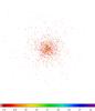Fig. 1 Simulated image of photon counts from a galaxy cluster with a mass of 5 × 1014h-1   M⊙, a redshift of 0.2, and an exposure time of 1000  s. The detected photons have energies in the range of 0.5 − 8 keV. The resolution of this image was lowered by a factor of 6 compared to the resolution of the simulated Chandra image for visibility.

The reconstructed and normalised gravitational potential φ is shown in Fig. 3a, together with the true potential that the clusters were modelled with. Despite the statistical fluctuations of the surface brightness profile supplied to the algorithm, the contribution of the background noise exceeds the real surface brightness profile at large radii (i.e. s ≳ 0.8h^-1Mpc), which then leads to an overestimation of the gravitational potential. This effect and the normalisation condition of the deprojection algorithm leads to a slight underestimation at smaller radii (i.e. s ≲ 0.3h^-1Mpc). However, as we are only interested in the lensing potential, major fluctuations are averaged out as seen in Fig. 3b.

3.2. Testing the algorithm

Next, we test the sensitivity of the potential reconstruction against changing certain parameters of the deprojection algorithm. We compare reconstructions of the X-ray emissivity obtained by assigning different weights α from [0.0,0.4,0.7,0.9] to the entropic regularisation term, with α = 0.0 corresponding to no regularisation, and constant L = 0.3h^-1Mpc. However, strong regularisation causes the reconstruction to overestimate the signal because of broad averaging by means of the flattening default kernel, because the regularisation penalises curvature. This can be seen at large radii.

A similar conclusion can be drawn from Fig. 4b, which contains the deprojected profile for different choices of the smoothing scale L from [0.1,0.3,0.7,0.9] h^-1Mpc while α = 0.4 is kept fixed. Thanks to the smoothing process performed by the floating default regularisation, a large fraction of the noise pattern, especially for large radii, is averaged out, which improves the convergence towards the expected result.

As a final test, we calculate the uncertainty of our reconstructed lensing potentials. We obtain this uncertainty by bootstrapping, sampling the synthetic cluster data N = 200 times, and applying our reconstruction algorithm. For each result of the reconstruction, the mean squared deviation from the true potential is calculated and then averaged over the number of bootstraps, giving the rms deviation: 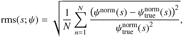$\mathrm{rms}\mathrm{\left(}\mathit{s}\mathrm{;}\mathit{\psi }\mathrm{\right)}\mathrm{=}\sqrt{\frac{\mathrm{1}}{\mathit{N}}\sum _{\mathit{n}\mathrm{=}\mathrm{1}}^{\mathit{N}}\frac{({\mathit{\psi }}^{\mathrm{norm}}\mathrm{\left(}\mathit{s}\mathrm{\right)}\mathrm{-}{\mathit{\psi }}_{\mathrm{true}}^{\mathrm{norm}}\mathrm{\left(}\mathit{s}\mathrm{\right)}{)}^{\mathrm{2}}}{{{\mathit{\psi }}_{\mathrm{true}}^{\mathrm{norm}}\mathrm{\left(}\mathit{s}\mathrm{\right)}}^{\mathrm{2}}}}\mathit{,}$(39)where quantities marked with a superscript “norm” are normalised to reach zero at the maximum projected radius. These rms are shown in the first panel of Fig. 5. Since this rms incorporates statistical, as well as systematic errors, we obtain a relative deviation from the true lensing potential of about 2% for high values of s. The relative rms increases with increasing radius due to the poorer signal.

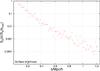Fig. 2 Azimuthally averaged and normalised surface brightness profile of a simulated galaxy cluster with a mass of 5 × 1014h-1   M⊙ and a redshift of 0.2. The corresponding synthetic observational data is shown in Fig. 1.

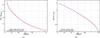Fig. 3 a) Reconstructed and normalised gravitational potential of a simulated galaxy cluster with a mass of 5 × 1014h-1   M⊙ and a redshift of 0.2. The potential was reconstructed assuming α = 0.4 and L = 0.3h-1Mpc. b) Corresponding lensing potential for this simulated cluster.

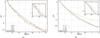Fig. 4 a) Comparison between different choices for the weights α of the penalty function in the reconstruction of the X-ray emissivity with constant smoothing scale L = 0.3h-1Mpc. The expected result based on Eq. (10) is plotted for reference, whereas α = 0.0 corresponds to no regularisation. b) Comparison between different choices of the smoothing scale of the regularisation function in the reconstruction of the X-ray emissivity and α = 0.4. The expected result is plotted for reference.

Since we also know the exact surface brightness of the cluster simulation, we can estimate the relative systematic error of the algorithm itself. Doing so, we bin the real surface brightness profile in the same way as we binned our statistical CCD images and obtain a reconstruction that does not inherit any statistical fluctuations or noise. We call this the best possible reconstruction ψ_ideal. Its rms with respect to the true lensing potential ψ_true provides an estimate for the systematic error of our reconstruction algorithm (shown in the lower panel of Fig. 5). This mean squared deviation increases slightly with the cluster radius, but always remains below 1.0%.

3.3. Deviations from spherical symmetry

As a last test we show how deviations from spherical symmetry affect our reconstruction algorithm. For this purpose we create a CCD image of a single subhalo with a mass of 1 × 10¹⁴h^-1   M_⊙ at redshift z_cl = 0.2, with a virial radius of r_subhalo ≈ 0.7h^-1   Mpc. We combine this CCD image with the simulated image of the cluster shown previously, with a projected distance of 0.5h^-1   Mpc between the two cluster centres. In a first-order approximation we accumulate the surface brightness of these two cluster realisations, before we apply our radial averaging scheme, again assuming spherical symmetry. Even though the subhalo is clearly visible in the lower panel of Fig. 5 (black arrow), we find that the maximum rms deviation of the lensing potential does not exceed the 2.0% deviation achieved without a subhalo. However, the reconstruction is rather insensitive to this kind of perturbation because of the radial averaging being applied to the input data. Further simulations show that the closer the subhalo lies in the centre of the hosting galaxy cluster, the less is the influence on the reconstruction, since the degree of asymmetry decreases.

4. Conclusions

This work is motivated by existing and upcoming observational data on galaxy clusters. A set of accurate tools to constrain fundamental cluster quantities is available: weak and strong gravitational lensing observations constrain the line-of-sight projection of the cluster potential, X-ray observations constrain the density and the temperature of the intracluster gas, while the Sunyaev-Zel’dovich effect constrains the gas pressure. A further constraint on the gradient of the gravitational potential can be found by means of galaxy kinematics. Our final goal is to combine all non-lensing information on clusters with existing lensing reconstruction methods (e.g. Bartelmann et al. 1996; Bradač et al. 2005, 2006; Cacciato et al. 2006; Merten et al. 2009).

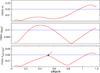Fig. 5 From top to bottom: rms deviation of ψ from ψtrue, rms deviation of ψideal from ψtrue and rms deviation of ψsubhalo from ψtrue, according to Eq. (39). Calculated from 200 realisations of a modelled galaxy cluster with a mass of 5 × 1014h-1   M⊙, a subhalo with mass 1 × 1014h-1   M⊙, and a redshift of 0.2. The blue lines represent a 2.0% and 1.0% threshold.

In this first paper in a planned series, we have outlined a non-parametric reconstruction method for the projected gravitational potential of galaxy clusters from thermal X-ray emission, assuming hydrostatic equilibrium and spherical symmetry. It is more cumbersome, but quite straightforward to extend this method to triaxial haloes. This extension is now being treated.

Our algorithm was laid out in Sect. 2. Assuming that the cluster is near or in hydrostatic equilibrium, we derived an analytic relation between the frequency-integrated bremsstrahlung emissivity and the three-dimensional Newtonian potential, Eq. (10). The algorithm deprojects the observed X-ray surface-brightness profile by means of the Richardson-Lucy method, converts it to the potential, and projects that.

Numerical tests show how this algorithm performs under reasonably realistic conditions and how sensitive it is to its parameters. We used one representative cluster realisation to obtain a realistic simulation of observational data. A comparison of different values of the weight α and the smoothing scale L of the regularisation term suggested that there is no significant variation in the final reconstruction of the X-ray emissivity if the floating default regularisation function is adopted with reasonable values.

Even though our simulated galaxy clusters have a rather smooth surface brightness profile, this technique can be applied without restrictions to less well-behaved observational data, e.g. strongly peaked emission in the cluster centre due to cooling effects. In such cases, the peaked centre could be masked and then passed to the Richardson-Lucy algorithm. The results would still be reliable thanks to the local character of the reconstruction scheme.

Furthermore, we determined the systematic error of our algorithm by applying it to ideally smooth rather than discretely sampled data to be at most 1.0%. We finally estimated the combination of systematic and statistical errors of our cluster-reconstruction algorithm to be at most 2.0% for s ≈ r_vir. Both rms were shown in Fig. 5.

We also addressed the problem of a galaxy cluster with an asymmetric surface brightness, e.g. containing a subhalo, in Sect. 3.3. Owing to azimuthal averaging, our reconstruction algorithm turns out to be rather insensitive to these kinds of perturbations.

Acknowledgments

This work was supported in part by contract research “Internationale Spitzenforschung II-1” of the Baden-Württemberg Stiftung, by the Collaborative Research Centre TR 33 and project BA 1369/17 of the Deutsche Forschungsgemeinschaft.

References

All Figures

	Fig. 1 Simulated image of photon counts from a galaxy cluster with a mass of 5 × 1014h-1   M⊙, a redshift of 0.2, and an exposure time of 1000  s. The detected photons have energies in the range of 0.5 − 8 keV. The resolution of this image was lowered by a factor of 6 compared to the resolution of the simulated Chandra image for visibility.
In the text

	Fig. 2 Azimuthally averaged and normalised surface brightness profile of a simulated galaxy cluster with a mass of 5 × 1014h-1   M⊙ and a redshift of 0.2. The corresponding synthetic observational data is shown in Fig. 1.
In the text

	Fig. 3 a) Reconstructed and normalised gravitational potential of a simulated galaxy cluster with a mass of 5 × 1014h-1   M⊙ and a redshift of 0.2. The potential was reconstructed assuming α = 0.4 and L = 0.3h-1Mpc. b) Corresponding lensing potential for this simulated cluster.
In the text

Fig. 4 a) Comparison between different choices for the weights α of the penalty function in the reconstruction of the X-ray emissivity with constant smoothing scale L = 0.3h-1Mpc. The expected result based on Eq. (10) is plotted for reference, whereas α = 0.0 corresponds to no regularisation. b) Comparison between different choices of the smoothing scale of the regularisation function in the reconstruction of the X-ray emissivity and α = 0.4. The expected result is plotted for reference.

In the text

	Fig. 5 From top to bottom: rms deviation of ψ from ψtrue, rms deviation of ψideal from ψtrue and rms deviation of ψsubhalo from ψtrue, according to Eq. (39). Calculated from 200 realisations of a modelled galaxy cluster with a mass of 5 × 1014h-1   M⊙, a subhalo with mass 1 × 1014h-1   M⊙, and a redshift of 0.2. The blue lines represent a 2.0% and 1.0% threshold.
In the text

References

- Bartelmann, M., Narayan, R., Seitz, S., & Schneider, P. 1996, ApJ, 464, L115 [NASA ADS] [CrossRef] [Google Scholar]
- Boylan-Kolchin, M., Springel, V., White, S. D. M., Jenkins, A., & Lemson, G. 2009, MNRAS, 398, 1150 [NASA ADS] [CrossRef] [Google Scholar]
- Bradač, M., Schneider, P., Lombardi, M., & Erben, T. 2005, A&A, 437, 39 [NASA ADS] [CrossRef] [EDP Sciences] [Google Scholar]
- Bradač, M., Clowe, D., Gonzalez, A. H., et al. 2006, ApJ, 652, 937 [NASA ADS] [CrossRef] [Google Scholar]
- Broadhurst, T., Umetsu, K., Medezinski, E., Oguri, M., & Rephaeli, Y. 2008, ApJ, 685, L9 [NASA ADS] [CrossRef] [Google Scholar]
- Cacciato, M., Bartelmann, M., Meneghetti, M., & Moscardini, L. 2006, A&A, 458, 349 [NASA ADS] [CrossRef] [EDP Sciences] [Google Scholar]
- Coe, D., Umetsu, K., Zitrin, A., et al. 2012, ApJ, 757, 22 [NASA ADS] [CrossRef] [Google Scholar]
- Finoguenov, A., Reiprich, T. H., & Böhringer, H. 2001, A&A, 368, 749 [NASA ADS] [CrossRef] [EDP Sciences] [Google Scholar]
- Gao, L., Frenk, C. S., Boylan-Kolchin, M., et al. 2011, MNRAS, 410, 2309 [NASA ADS] [CrossRef] [Google Scholar]
- Horne, K. 1985, in Interacting Binaries, eds. P. P. Eggleton, & J. E. Pringle, NATO ASIC Proc., 150, 327 [Google Scholar]
- Lahav, O., & Gull, S. F. 1989, MNRAS, 240, 753 [NASA ADS] [Google Scholar]
- Lucy, L. B. 1974, AJ, 79, 745 [NASA ADS] [CrossRef] [Google Scholar]
- Lucy, L. B. 1994, A&A, 289, 983 [NASA ADS] [Google Scholar]
- Merten, J., Cacciato, M., Meneghetti, M., Mignone, C., & Bartelmann, M. 2009, A&A, 500, 681 [NASA ADS] [CrossRef] [EDP Sciences] [Google Scholar]
- Narayan, R., & Nityananda, R. 1986, ARA&A, 24, 127 [NASA ADS] [CrossRef] [Google Scholar]
- Navarro, J. F., Frenk, C. S., & White, S. D. M. 1997, ApJ, 490, 493 [NASA ADS] [CrossRef] [Google Scholar]