© ESO, 2013

1. Introduction

The first maser signal was detected in 1965 (Weaver et al. 1965). It was produced by OH and the intriguing nature of this detection was rapidly attributed to a non-thermal phenomenon (Davies et al. 1967) which originates in the amplification of the radiation due to stimulated emission. Since then, many improvements have been made both in observational facilities and maser theory, leading to an abundant literature on the subject. The main results, both theoretical and observational, have been summarised by, for example, Elitzur (1992) or Gray (1999). Major improvements in observational techniques have been made in the last 20 years thanks to the rise of sensitive interferometers and very-long-baseline interferometer (VLBI) techniques (see e.g. Humphreys 2007; Fish 2007, and references therein). The sizes of the regions where maser emission is detected have typical scales of a few AU. Nevertheless, some masers arise from large spatial scales, such as the 183.3 GHz line of water vapour (Cernicharo et al. 1990, 1994). Despite the fact that, theoretically, many improvements have been made in explaining the pumping mechanisms of molecular masers, there are no definitive explanations that account for all the observations as yet. As an example, the problem of water megamasers observed in the direction of active galactic nuclei (AGN) is still a subject of debate (Elitzur et al. 1989; Deguchi & Watson 1989; Kylafis & Pavlakis 1999; Cernicharo et al. 2006a).

The basics of the standard maser theory which is widely used to interpret masing lines have been reviewed by Elitzur (1992). The main aspect of this theory is to introduce the effect of saturation which puts limits on the amount of energy that can be radiated by a masing line. As outlined by Collison & Nedoluha (1995), theoretical studies of masers adopt two different strategies: i) they solve exactly the radiative transfer in the maser but with a simplified description of the energy levels of the molecule; ii) they deal with an exact description of the molecule but with approximations in the radiative transfer treatment. In the latter case, the escape probability formalism is widely used, despite the fact that the validity of this approximation is questionable in the case of masing lines. Indeed, intense masers require a large amplification path and, therefore, coherence in velocity over relatively large scales. In contrast, the basic principle of the large velocity gradient (LVG) approximation is that the different regions of the cloud are decoupled through Doppler shifting, hence limiting the coherence path. In this work we present a self-consistent method that aims to go beyond the approximations usually made, i.e. we present a method that enables us to solve exactly the radiative transfer problem and in which we deal with a rigorous description of the molecule.

The theory relevant to the description of masing lines which also shows how the radiative transfer is solved is described in Sect. 2. An application for the o–H₂O molecule is presented in Sect. 3 where the method developed in this study is compared to other less accurate approaches. Finally, the current method is used in Sect. 4 in order to predict which lines of o–H₂O or p–H₂O could be inverted for densities and temperatures typical of AGB circumstellar envelopes. In this section, the predictions based on various sets of collisional rate coefficients involving He, p–H₂, or o–H₂ are also compared.

2. Theory

2.1. Absorption coefficient

In the case of intense masers, the radiation field starts to influence the inversion of the population, avoiding a complete frequency redistribution, leading to differing line profiles for absorption and emission. This occurs when the intensity in the masing lines exceeds a certain threshold which depends on the given physical conditions. In this case, the maser is said to be saturated. The way this effect is introduced in the theory is described later in this section.

Under a particular geometry the amplification path varies with direction, implying that the distribution of molecular velocities should in principle be considered as anisotropic. This problem was first identified by Bettwieser & Kegel (1974). In the case of spherical geometry, a common approximation, known as “standard theory”, consists of neglecting the anisotropy of the molecular velocities resulting from the existence of directions of different path lengths. The validity of this assumption was tested in various studies (see e.g. Bettwieser 1976; Neufeld 1992; Emmering & Watson 1994; Elitzur 1994) for spherical geometry. They concluded that considering explicitly the anisotropies of the absorption coefficient could lead to variations in the properties of the emerging maser radiation in the case of saturated masers. However, it was pointed out that these variations remain unimportant in comparison to the uncertainties that affect maser theory, and that the standard theory should be a reasonably good first approximation. Given the large number of simplifications adopted by the standard theory in the treatment of the radiative transfer (RT), we assume in the following that the masing-line absorption coefficients are isotropic, and we follow a procedure similar to that described by Anderson & Watson (1993). First, we consider the frequency-dependent statistical equilibrium equations (SEE) for the level i: $\begin{array}{ccc}\frac{\mathrm{d}{\mathit{n}}_{\mathit{i}}\mathrm{\left(}\mathit{v}\mathrm{\right)}}{\mathrm{d}\mathit{t}}& \mathrm{=}& \sum _{\mathit{j}\ne \mathit{i}}\mathrm{[}{\mathit{N}}_{\mathit{j}}\hspace{0.17em}\mathit{\phi }\mathrm{\left(}\mathit{v}\mathrm{\right)}{\mathit{C}}_{\mathit{ji}}\mathrm{-}{\mathit{n}}_{\mathit{i}}\mathrm{\left(}\mathit{v}\mathrm{\right)}{\mathit{C}}_{\mathit{ij}}\mathrm{]}\mathrm{+}\left[{\mathit{N}}_{\mathit{i}}\hspace{0.17em}\mathit{\phi }\mathrm{\left(}\mathit{v}\mathrm{\right)}\mathrm{-}{\mathit{n}}_{\mathit{i}}\mathrm{\left(}\mathit{v}\mathrm{\right)}\right]{\mathit{C}}_{\mathit{ii}}\\ & & \end{array}$(1)with $\begin{array}{ccc}\begin{array}{c}\\ \end{array}& & \end{array}$(2)In these equations, N_j represents the total population of level j, n_j(v) is the population of level j at the velocity v. The quantity φ(ν) corresponds to the usual Doppler line profile that accounts for both the thermal and turbulent motion of the molecules, A_ij and B_ij are the Einstein coefficients for spontaneous and induced emission, E_j is the energy of level j, C_ji are the collisional rates from level j to level i, and I_v(Ω) is the specific intensity in a direction specified by Ω. We note that in Eq. (1) the elastic collisional rates C_ii have to be formally included since they contribute to the relaxation of velocities (Anderson & Watson 1993). Equation (1) can be re-written so that all levels except those involving the maser transition are included in the so-called pump and loss rates. This leads to a phenomenological treatment where the full SEE is artificially reduced to a two-level system. In the following, the labels u and l indicate the upper and lower maser levels. Assuming that for all the other transitions the absorption and emission line profiles are identical and are given by the Doppler line profile φ(ν), we obtain from Eq. (1) $\begin{array}{ccc}\mathrm{0}& \mathrm{=}& {\mathrm{\Lambda }}_{\mathit{u}}\mathrm{\left(}\mathit{v}\mathrm{\right)}\hspace{0.17em}\mathit{\phi }\mathrm{\left(}\mathit{v}\mathrm{\right)}\mathrm{-}{\mathit{n}}_{\mathit{u}}\mathrm{\left(}\mathit{v}\mathrm{\right)}\left[{\mathrm{\Gamma }}_{\mathit{u}}\mathrm{\left(}\mathit{v}\mathrm{\right)}\mathrm{+}{\mathit{C}}_{\mathit{ul}}\mathrm{+}{\mathit{C}}_{\mathit{uu}}\right]\\ & & \\ \mathrm{0}& \mathrm{=}& {\mathrm{\Lambda }}_{\mathit{l}}\mathrm{\left(}\mathit{v}\mathrm{\right)}\hspace{0.17em}\mathit{\phi }\mathrm{\left(}\mathit{v}\mathrm{\right)}\mathrm{-}{\mathit{n}}_{\mathit{l}}\mathrm{\left(}\mathit{v}\mathrm{\right)}\left[{\mathrm{\Gamma }}_{\mathit{l}}\mathrm{\left(}\mathit{v}\mathrm{\right)}\mathrm{+}{\mathit{C}}_{\mathit{lu}}\mathrm{+}{\mathit{C}}_{\mathit{ll}}\right]\\ & & \end{array}$where the pump and loss rates, noted Λ_i and Γ_i (with i ∈  { u,l }), are defined by $\begin{array}{ccc}{\mathrm{\Lambda }}_{\mathit{i}}\mathrm{\left(}\mathit{v}\mathrm{\right)}& \mathrm{=}& \sum _{\mathit{j}\ne \mathrm{\left\{}\mathit{u,l}\mathrm{\right\}}}{\mathit{N}}_{\mathit{j}}\hspace{0.17em}\mathrm{[}{\mathit{C}}_{\mathit{ji}}\mathrm{+}{\mathit{R}}_{\mathit{ji}}\mathrm{(}\mathit{v}{\mathrm{)}}^{\mathrm{]}}\\ {\mathrm{\Gamma }}_{\mathit{i}}\mathrm{\left(}\mathit{v}\mathrm{\right)}& \mathrm{=}& \sum _{\mathit{j}\ne \mathrm{\left\{}\mathit{u,l}\mathrm{\right\}}}\mathrm{[}{\mathit{C}}_{\mathit{ij}}\mathrm{+}{\mathit{R}}_{\mathit{ij}}\mathrm{(}\mathit{v}{\mathrm{)}}^{\mathrm{]}}\mathit{.}\end{array}$This leads to the usual expression $\begin{array}{ccc}\mathrm{\Delta }\mathit{n}\mathrm{\left(}\mathit{v}\mathrm{\right)}\mathrm{=}\frac{{\mathit{g}}_{\mathit{l}}}{{\mathit{g}}_{\mathit{u}}}\hspace{0.17em}{\mathit{n}}_{\mathit{u}}\mathrm{\left(}\mathit{v}\mathrm{\right)}\mathrm{-}{\mathit{n}}_{\mathit{l}}\mathrm{\left(}\mathit{v}\mathrm{\right)}\mathrm{=}{\mathit{n}}_{\mathrm{0}}\mathrm{\left(}\mathit{v}\mathrm{\right)}\hspace{0.17em}{\left[\mathrm{1}\mathrm{+}\frac{{\mathit{R}}_{\mathit{lu}}\mathrm{\left(}\mathit{v}\mathrm{\right)}}{\mathit{J̅}\mathrm{\left(}\mathit{v}\mathrm{\right)}}\right]}^{-1}\hspace{0.17em}\mathit{\phi }\mathrm{\left(}\mathit{v}\mathrm{\right)}& & \end{array}$(7)with $\begin{array}{ccc}{\mathit{n}}_{\mathrm{0}}\mathrm{\left(}\mathit{v}\mathrm{\right)}& \mathrm{=}& \frac{\mathrm{1}}{\mathrm{1}\mathrm{+}\mathrm{ℬ}\mathrm{\left(}\mathit{v}\mathrm{\right)}\frac{{\mathit{g}}_{\mathit{u}}}{{\mathit{g}}_{\mathit{l}}}{\mathit{A}}_{\mathit{ul}}}\hspace{0.17em}(\mathrm{𝒜}\mathrm{\left(}\mathit{v}\mathrm{\right)}\left[{\mathrm{\Lambda }}_{\mathit{u}}\mathrm{\left(}\mathit{v}\mathrm{\right)}\mathrm{+}{\mathit{N}}_{\mathit{l}}\hspace{0.17em}{\mathit{C}}_{\mathit{lu}}\mathrm{+}{\mathit{N}}_{\mathit{u}}\hspace{0.17em}{\mathit{C}}_{\mathit{uu}}\right]{}^{}\\ & & \mathrm{-}\hspace{0.17em}{}^{}\mathrm{ℬ}\mathrm{\left(}\mathit{v}\mathrm{\right)}\left[{\mathrm{\Lambda }}_{\mathit{l}}\mathrm{\left(}\mathit{v}\mathrm{\right)}\mathrm{+}{\mathit{N}}_{\mathit{u}}\hspace{0.17em}{\mathit{C}}_{\mathit{ul}}\mathrm{+}{\mathit{N}}_{\mathit{l}}\hspace{0.17em}{\mathit{C}}_{\mathit{ll}}\right])\\ \mathit{J̅}\mathrm{\left(}\mathit{v}\mathrm{\right)}& \mathrm{=}& \end{array}$and $\begin{array}{ccc}\mathrm{𝒜}\mathrm{\left(}\mathit{v}\mathrm{\right)}& \mathrm{=}& \frac{{\mathit{g}}_{\mathit{l}}}{{\mathit{g}}_{\mathit{u}}}{\left[{\mathrm{\Gamma }}_{\mathit{u}}\mathrm{\left(}\mathit{v}\mathrm{\right)}\mathrm{+}{\mathit{C}}_{\mathit{ul}}\mathrm{+}{\mathit{C}}_{\mathit{uu}}\mathrm{+}{\mathit{A}}_{\mathit{ul}}\right]}^{-1}\\ \mathrm{ℬ}\mathrm{\left(}\mathit{v}\mathrm{\right)}& \mathrm{=}& {\left[{\mathrm{\Gamma }}_{\mathit{l}}\mathrm{\left(}\mathit{v}\mathrm{\right)}\mathrm{+}{\mathit{C}}_{\mathit{lu}}\mathrm{+}{\mathit{C}}_{\mathit{ll}}\mathrm{-}\frac{{\mathit{g}}_{\mathit{u}}}{{\mathit{g}}_{\mathit{l}}}{\mathit{A}}_{\mathit{ul}}\right]}^{-1}\mathit{.}\end{array}$The source function of the masing line is given by 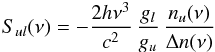$\begin{array}{ccc}{\mathit{S}}_{\mathit{ul}}\mathrm{\left(}\mathit{\nu }\mathrm{\right)}\mathrm{=}\mathrm{-}\frac{\mathrm{2}\mathit{h}{\mathit{\nu }}^{\mathrm{3}}}{{\mathit{c}}^{\mathrm{2}}}\hspace{0.17em}\frac{{\mathit{g}}_{\mathit{l}}}{{\mathit{g}}_{\mathit{u}}}\hspace{0.17em}\frac{{\mathit{n}}_{\mathit{u}}\mathrm{\left(}\mathit{\nu }\mathrm{\right)}}{\mathrm{\Delta }\mathit{n}\mathrm{\left(}\mathit{\nu }\mathrm{\right)}}& & \end{array}$(12)where n_u(ν) can be obtained from Eqs. (3) and (7). Contrary to the case of thermal lines, the source function is frequency dependent for the maser line.

To obtain the source functions and the absorption coefficients from these expressions, we see that the relevant quantities are the specific line intensities (averaged over the angles) and the total level populations N_j. The latter are obtained by solving the frequency independent SEE expressed by $\begin{array}{ccc}\mathrm{0}& \mathrm{=}& \end{array}$(13)with $\begin{array}{ccc}\mathit{J̅}\mathit{kl}\mathrm{=}\mathrm{\int }{\mathit{\phi }}_{\mathit{k}}\mathrm{\left(}\mathit{\nu }\mathrm{\right)}\hspace{0.17em}{\mathit{R}}_{\mathit{kl}}\mathrm{\left(}\mathit{\nu }\mathrm{\right)}\hspace{0.17em}\mathrm{d}\mathit{\nu }\mathit{.}& & \end{array}$(14)In the last expression, the velocity profile φ_k(ν) = n_k(ν)/N_k accounts for the departure from the Doppler line profile if the line k → l is a masing transition, for consistency with Eq. (1). In the case of thermal lines, these profiles are simply given by the Doppler profile and are identical for both levels; the average of the specific intensities over angles and velocities in Eq. (13) can be factorized, which is crucial in establishing the preconditioned form of the SEE, as discussed by Rybicki & Hummer (1991). In the case of masing lines and for consistency with Eq. (1), we have introduced unequal velocity profiles for the maser levels; consequently the factorisation leading to the preconditioned SEE is no longer feasible. Hence, the usual approximated lambda iteration (ALI) method cannot be applied.

In most studies treating the radiative transfer in the presence of masers, the pumping rates are taken to be independent of the velocity. In this case the expression for the population difference is similar to Eq. (7) except that the velocity dependence of n₀(ν) and is omitted. Hence, the absorption coefficient will depend only on velocity through the term R_lu(ν). In the case of unsaturated masers, this term is always negligible in comparison to and the absorption coefficient is given by the Doppler line profile. However, for a saturated maser, i.e. for a line with , the absorption coefficient decreases at the line centre. This translates to the fact that, for a given pumping scheme, the molecules pumped to the upper level are readily depleted to the lower by stimulated emission since the number of masing photons is large. At this stage the maser amplification starts to be linear at the line centre and the maser line re-broadens.

2.2. Solution of the transfer equation

To solve the transfer equation we have used the short characteristic (SC) method introduced by Olson & Kunasz (1987). The numerical code based on this method has previously been described in Daniel & Cernicharo (2008) for the case of thermal transitions in 1D spherical geometry. Briefly, in the SC method we assume that the source function can be reproduced numerically by a polynomial function of the opacity in the line (usually of polynomial degree 1 or 2). At each iteration the absorption coefficients are known from the current populations, and the opacities are evaluated assuming that they behave linearly between consecutive grid points. These assumptions permit us to solve analytically the transfer equation at each spatial grid point. In our models, the radiative transfer deals with both maser and thermal lines. However, the treatment for maser propagation is only switched on when the opacity of a line τ_ul = N_l − g_l/g_u   N_u at a particular grid point is negative. For the same line and for the radii where the opacity is positive, the line is treated in a standard way relevant to thermal radiation.

In what follows we describe a method that allows us to solve the transfer equation for masing lines. It is based on the assumption that the source functions are linearly interpolated. Hence, along a characteristic, specific intensities are derived according to $\begin{array}{ccc}{\mathit{I}}_{\mathit{i}}& \mathrm{=}& \end{array}$(15)where the α_i and β_i coefficients depend on the opacity Δ   τ_i between points i and i − 1.

In the case of masing lines, a difficulty arises from the fact that the absorption coefficient at point i depends on the angular average R_lu(v) of the specific intensities I_i(θ) $\begin{array}{ccc}{\mathit{\kappa }}_{\mathit{lu}}\mathrm{\left(}\mathit{v}\mathrm{\right)}\mathrm{=}\mathrm{-}\frac{\mathit{h\nu }}{\mathrm{4}\hspace{0.17em}\mathit{\pi }}{\mathit{B}}_{\mathit{lu}}\hspace{0.17em}{\mathit{n}}_{\mathrm{0}}^{\mathrm{+}}\mathrm{\left(}\mathit{v}\mathrm{\right)}\hspace{0.17em}{\left[\mathrm{1}\mathrm{+}\frac{{\mathit{R}}_{\mathit{lu}}\mathrm{\left(}\mathit{v}\mathrm{\right)}}{\mathit{J̅}\mathrm{+}\mathrm{\left(}\mathit{v}\mathrm{\right)}}\right]}^{-1}\hspace{0.17em}\mathit{\phi }\mathrm{\left(}\mathit{v}\mathrm{\right)}\mathit{,}& & \end{array}$(16)where the quantities indexed by a cross (e.g. ) are obtained with the current estimate for the populations of the energy levels (i.e. the populations obtained at the previous iteration). The same applies to the source functions (see Eq. (12)). Therefore, the radiative transfer equation becomes integro-differential, whereas in the case of thermal lines, the problem consists in solving a differential equation. Note that the integral part of this integro-differential equation involves an integration of the intensities over 4π steradians. In order to obtain intensities which are fully self-consistent with the level populations used at a given iteration, we proceed in three steps.

2.2.1. First iterative scheme

As a first step, we derive specific intensities at each grid point according to Eq. (15), assuming that the source functions are independent of the radiation field. In other words, we use Eq. (12) in order to express the source function assuming that the average radiation field is ${\mathit{R}}_{\mathit{lu}}^{\mathrm{+}}\mathrm{\left(}\mathit{\nu }\mathrm{\right)}$. For each frequency, we obtain the solution iteratively by calculating I_v(θ) for θ ∈  [0:π] and then updating κ_lu(v) at grid point i. We iterate until the calculated specific intensities are consistent with the initial averaged radiation field.

In the following discussion, R_lu(ν) is indexed by i or f whenever it corresponds to the radiation field used in the evaluation of κ_lu(ν) or to the one which results from the evaluation of Eq. (15) and made use of ${\mathit{R}}_{\mathit{lu}}^{\mathit{i}}\mathrm{\left(}\mathit{\nu }\mathrm{\right)}$. Additionally, the solutions obtained during the previous steps are indexed with the superscript > if they satisfy ${\mathit{R}}_{\mathit{lu}}^{\mathit{f}}\mathrm{\left(}\mathit{\nu }\mathrm{\right)}\mathit{>}{\mathit{R}}_{\mathit{lu}}^{\mathit{i}}\mathrm{\left(}\mathit{\nu }\mathrm{\right)}$ and with the superscript < if they do not. Once the iterative process has been initialised, a trial value for R_lu(v) is obtained according to $\begin{array}{ccc}\log {\mathit{R}}_{\mathit{lu}}\mathrm{\left(}\mathit{\nu }\mathrm{\right)}\mathrm{=}\frac{\mathit{b}}{\mathrm{1}\mathrm{-}\mathit{a}}& & \end{array}$(17)with $\begin{array}{ccc}\{\begin{array}{c}\\ & & \\ & & \\ & & \end{array}& & \end{array}$(18)The radiation field derived in this way is used to update κ_lu(ν). Depending on the resulting specific intensities, one of the pair (${\mathit{R}}_{\mathit{lu}}^{\mathit{i}\mathit{>}}$, ${\mathit{R}}_{\mathit{lu}}^{\mathit{f}\mathit{>}}$) or (${\mathit{R}}_{\mathit{lu}}^{\mathit{i}\mathit{<}}$, ${\mathit{R}}_{\mathit{lu}}^{\mathit{f}\mathit{<}}$) is updated. Finally, the iterative process is stopped when we have ${\mathit{R}}_{\mathit{lu}}^{\mathit{i}}\mathrm{=}{\mathit{R}}_{\mathit{lu}}^{\mathit{f}}$ within a given accuracy. Figure 1 shows the typical behaviour of ${\mathit{R}}_{\mathit{lu}}^{\mathit{f}}$ as a function of ${\mathit{R}}_{\mathit{lu}}^{\mathit{i}}$. The averaged radiation fields determined using our method are marked with squares and are indexed according to the iteration number.

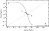Fig. 1 Variation of the averaged radiation field (solid line) as a function of the initial radiation field entering in the determination of the absorption coefficient. The dashed line corresponds to a straight line of slope unity. The solution of the problem corresponds to the intersection between the two curves. The squares correspond to the averaged radiation field obtained at each iteration.

2.2.2. Second iterative scheme

Once this process has been completed, we perform an update of the source function at point i according to Eq. (12), using the average radiation field R_lu(ν) derived during the first iterative scheme. The whole process is then repeated until we obtain convergence for the source function at the current grid point.

2.2.3. Third iterative scheme

As previously stated, in order to derive the absorption coefficient, it is necessary to know the angular average of specific intensities over 4π sr. Using the SC method, the spatial grid is first swept from the outermost grid point (i = N) to the innermost one (i = 1) providing the intensities I_i(θ) with i ∈  [1;N] and θ ∈  [π/2;π]). The grid is then swept in the other direction so that the intensities for θ ∈  [0;π/2]) are then known. This sweeping procedure is adopted so that at every moment during the propagation only the populations used at the current iteration are needed to derive the intensities. In the case of masing lines, an additional complexity arises from the fact that during the inward propagation, the incoming intensities for θ < θ_lim have not yet been calculated (cf. Fig. 2) with the current populations while they enter in the evaluation of the absorption coefficient.

The third iterative scheme thus consists of obtaining an overall convergence for the intensities I_i(θ) with i ∈  [1;N] and θ ∈  [0;π]. This is done by performing successive sweeping of the spatial grid, each iteration leading to an update of the intensities I_i(θ).

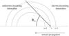Fig. 2 Schematic diagram showing the availability of incoming intensities during the inward propagation.

3. Application

To test our method, we have performed model calculations for the ortho state of the water molecule and the comparison is made with respect to a simplified treatment that aims to describe the masing lines. This simplified treatment relies on the assumption that the calculation of maser inversion and the resulting intensities can be achieved in a two-step procedure. First, the populations of the molecular levels are determined neglecting the specificity of maser radiative transfer. Secondly, the intensities of the masing lines are calculated using the populations obtained during the first step and taking into account maser propagation. This procedure has been used in previous studies (e.g. Yates et al. 1997; Watson et al. 2002) and the way it is presently implemented is described in the next sections.

The models consist of clouds of uniform H₂ density, temperature (assumed to be 400 K in all models), and o–H₂O abundance (40 levels have been considered). We have adopted a diameter of 4 × 10¹⁴ cm (2.6    ×    10^-4 pc) for the cloud which is the typical size of bright maser spots in the 22 GHz line of water. Moreover, this size provides a maximum amplification path similar to that of the slab depths used in Yates et al. (1997). The collisional rate coefficients are for the collisional system H₂O/He (Green et al. 1993) and are corrected to account for the different reduced masses of the H₂O/H₂ and H₂O/He systems. We have selected these rates rather than those of Dubernet et al. (2009) or Faure et al. (2007) as they were the ones used by Yates et al. (1997). These parameters being fixed, we performed the calculations in the (n(H₂), X(H₂O)) plane of parameter space with respective values in the range [2    ×    10⁵;8    ×    10⁹] cm^-3 and [2    ×    10^-6;8    ×    10^-4]. The accuracy of the results will depend on the gridding adopted. Typically, convergence is reached when the spatial sampling is such that the opacity between two consecutive grid points is around one or less. For all the calculations presented here, we adopted a grid with 500 spatial grid points, which might be inadequate for the highest densities/abundances considered here. However, since the masing lines are collisionally quenched at these densities/abundances, the effect of limited convergence accuracy does not affect our conclusions. Moreover, the main goal is to compare the effect of the radiative transfer and both model calculations are performed with the same spatial grid.

As presented in Sect. 2, elastic collisional rate coefficients for the levels involved in masing lines enter in the definition of the absorption coefficients and source functions. Test calculations have been performed by Anderson & Watson (1993) to test the influence of these rates and they concluded that in most cases their inclusion produces rather small effects. Hence, in the present test calculations, we have assumed that the elastic rate coefficients are set to zero. In other words, in the following calculations we assume that C_ii = 0 in Eq. (13), which subsequently alter the definition of the pump and loss rates. However, this is not a pre-requisite of the method and the elastic rate coefficients could be taken into account, if known. Moreover, despite of this, the effect of velocity redistribution is still present through the inelastic collisions terms and through the radiative terms associated to transitions which are connected either to the upper or lower energy level of the masing line under consideration.

3.1. Pumping scheme with and without maser propagation

As a first step, we compare the results of the exact calculation to a simplified treatment that consists of neglecting the amplification inherent to maser propagation when deriving the population of the energy levels of the molecule. To do this, we take the absolute value of the level population difference which then enters in the definition of the absorption coefficients and source functions. These quantities are defined with the usual expressions which are suitable for thermal lines. This permits us to treat masing lines in the same manner as thermal lines. This approach was previously adopted in plane parallel non-local calculations by Yates et al. (1997) with the aim of predicting which water lines could show maser excitation. Their results are discussed in terms of the gain in the masing lines (see Eq. (3) of Yates et al. 1997) 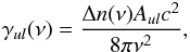$\begin{array}{ccc}{\mathit{\gamma }}_{\mathit{ul}}\mathrm{\left(}\mathit{\nu }\mathrm{\right)}\mathrm{=}\frac{\mathrm{\Delta }\mathit{n}\mathrm{\left(}\mathit{\nu }\mathrm{\right)}{\mathit{A}}_{\mathit{ul}}{\mathit{c}}^{\mathrm{2}}}{\mathrm{8}\mathit{\pi }{\mathit{\nu }}^{\mathrm{2}}}\mathit{,}& & \end{array}$(19)which is subsequently averaged over the slab depths (the so-called depth-weighted gain coefficient defined by Eq. (7) of Yates et al. 1997). Since γ_ul(ν) is proportional to the absorption coefficient κ_lu(ν), it is equivalent to consider either the depth-weighted gain coefficient or the opacity in the masing line, and in the following we choose to discuss the results in terms of line opacities. We emphasise the fact that at this stage the approximate method described here does not involve any treatment specific to maser radiation and that could account for saturation effects. Thus, the dependence on frequency of the population difference Δn(ν) which enters in the definition of γ_ul(ν) [or κ_lu(ν)] is given by the Doppler line profile φ(ν).

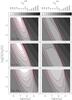Fig. 3 Isocontours of the o–H2O opacities at line centre for the 616 − 523 line at 22 GHz, the 414 − 321 line at 380 GHz, and the 423 − 330 line at 448 GHz. The left column corresponds to the models where the treatment of maser propagation is omitted and the right column to the current results (see text). The isocontour values and the correspondence between grey scale and opacity values are displayed at the top of the two columns. The isocontours that correspond to opacities of − 4 and − 40 are displayed in thick blue lines. Negative values for the opacity correspond to red lines.

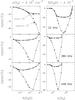Fig. 4 Comparison between the opacities derived with (solid lines) or without (dashed lines) accounting for maser propagation for the masers at 22 GHz, 380 GHz, and 448 GHz. The left column corresponds to a cut in density at n(H2) = 2    ×    107 cm-3; the differences are shown with respect to variations in X(H2O). The right column corresponds to a fixed water abundance, i.e. X(H2O) = 4    ×    10-4.

Figure 3 shows the opacity at line centre of the 22 GHz (6₁₆ − 5₂₃), 380 GHz (4₁₄–3₂₁), and 448 GHz (4₂₃–3₃₀) masing lines, obtained in the two treatments (labelled respectively on or off according to whether maser propagation is accounted for or not). Figure 4 shows the line opacities for the same lines with respect to cuts in density or H₂O abundance. We can see in these figures that including the current maser propagation treatment leads to a substantial decrease in the predicted line opacities for these lines. Indeed, without treating the exact radiation field in the masing lines, we obtain minimum optical depths of the order of − 70 for the 22 GHz line and − 40 for the 380 and 448 GHz transitions. With our method, the minimum optical depth for the 22 GHz line is reduced to − 20 and to − 5 for the other two lines.

3.2. Two-level maser propagation

To infer the influence of these changes in line opacities, we now consider the resulting masing-line intensities. To do this, any reasonable approximated treatment should include an RT theory that accounts for saturation effects. To obtain a reference point for the current results we compute the pump and loss rates Λ_i(v) and Γ_i(v) from the populations previously obtained in the approximate treatment. These values enter in the definition of the population difference Δn(v) through Eq. (7). Then, for a given masing line, the intensities are computed by adjusting R_lu(v) as described in Sect. 2.

Using this approximation, we obtain line intensities that differ largely from those obtained with the exact treatment described in Sect. 2. This is illustrated in Fig. 5 for the 22 GHz line. This figure shows the brightness temperatures obtained in the two treatments at a density n(H₂) = 4    ×    10⁷ cm^-3, for the centre of the line and for a line of sight that passes through the centre of the sphere. This figure shows that for water abundances X(H₂O) > 5    ×    10^-5 the approximate treatment leads to intensities larger by two orders of magnitude. This originates from the opacity overestimation obtained in the approximate treatment which was discussed in the previous section. Figure 6 compares the line profiles computed in the two treatments for the model with n(H₂) = 4    ×    10⁷ cm^-3 and X(H₂O) = 6    ×    10^-4. In this figure we see that the higher intensity found in the approximate treatment is accompanied by a broader line profile. This result is produced by the higher line saturation obtained in the approximate treatment with respect to the exact treatment. This fact is illustrated in Fig. 7 where the ratio is plotted as a function of the velocity offset to line centre and of the normalised radius in the cloud for the 22 GHz line, for both the exact and approximated methods. The parameters of the model are n(H₂) = 4    ×    10⁷ cm^-3 and X(H₂O) = 6    ×    10^-4. We see in this figure that in the exact calculation the degree of saturation is low, i.e. at any radii. In contrast, the saturation is high in the approximate calculation with at most radii.

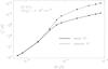Fig. 5 Brightness temperatures for the 22 GHz line obtained with the exact treatment (solid lines) and with the approximated treatment (dashed lines). The intensities correspond to a line of sight that crosses the centre of the sphere and are given for the rest frequency of the line.

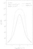Fig. 6 Emerging brightness temperature of the 22 GHz line for the model with n(H2) = 4    ×    107 and X(H2O) = 6    ×    10-4. The solid line corresponds to the intensity predicted by the exact calculation, the dashed line to the intensity predicted by the approximated RT (see text).

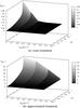Fig. 7 Ratio as a function of the offset to line centre and of the normalized radius in the cloud. This ratio is given for the 22 GHz line and corresponds to the model with n(H2) = 4    ×    107 and X(H2O) = 6 × 10-4. The two plots correspond to a) the exact treatment and b) an approximated treatment (see text).

In the exact treatment, the masing-line intensities are taken into account when deriving the populations, therefore the population difference between the upper and lower level of the masing line tends to be reduced by induced radiative de-excitation. Conversely, in the approximate treatment the averaged radiation field is largely underestimated. This means that the amount of induced radiative de-excitation events is underestimated, which leads to a greater difference between the populations of the lower and upper levels. Consequently, the derived masing-line opacity is larger and is accompanied by a larger degree of saturation of the line. So, the differences encountered in the two treatments originate in the overall flow of population from the upper to the lower level, which is induced by radiative de-excitation. The evaluation of this flow of population differs in the two treatments since it relies on the accuracy of the determination of the intensities in the masing line.

We note that in Sect. 2, Eq. (7) is derived from the velocity-dependent SEE and from this expression it is seen that an increase in the average radiation field leads to a decrease in Δn(ν). From similar considerations dealing with the velocity-independent SEE, it can be seen that increasing the value of the radiation field for the maser transitions would lead to lower population differences for the levels involved in the maser transitions. This behaviour is not a specific case and we can infer from it that considering maser propagation explicitly will necessarily lead to a decrease in line optical depths in comparison to treatments where the average radiation field would be underestimated.

3.3. Thermal lines

The two treatments for maser propagation differ in the evaluation of the average radiation field of the masing lines. Considering the current maser propagation treatment leads to higher values for the average radiation field which, in turn, when inverting the SEE, leads to a diminution in the population differences between levels involved in maser transitions. The modification of the populations of these levels subsequently modifies the whole energy level populations. This is illustrated in Fig. 8 for three lines which only show purely thermal emission. In this figure, we see that the opacities of these lines are modified and can show variations up to ~25% between the two treatments in the region of the (n(H₂), X(H₂O)) plane where maser transitions are the most opaque. Nevertheless, for the range of parameters considered here, the number of lines which suffer from optical depth variations greater than 10% is low, and for the majority of the thermal lines the opacities agree within a few percent points between the two treatments.

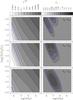Fig. 8 The left column corresponds to the opacity of three purely thermal lines obtained in a treatment where masing lines are treated explicitly. The right column corresponds to the ratio rτ = τoff/τon of the opacities obtained with the two treatments (see text).

4. Maser prediction

Most of the information that can be extracted from water line observations relies on the modelling of its excitation. However, water is a difficult molecule to treat since its high dipole moment causes most of its transitions to be sub-thermally excited (see e.g. Cernicharo et al. 2006b). The transitions harbour very large opacities (see e.g. González-Alfonso et al. 1998), and many of the transitions are maser in nature (Cheung et al. 1969; Waters et al. 1980; Phillips et al. 1980; Menten et al. 1990a,b; Menten & Melnick 1991; Cernicharo et al. 1990, 1994, 1996, 1999, 2006b; González-Alfonso et al. 1995, 1998). Accurate modelling thus requires, in addition to a good description of the source structure, the availability of collisional rate coefficients. Moreover, as discussed above, special formalisms have to be developed in order to have a realistic treatment of the transfer of radiation in the case of saturated masers. The method developed in the present work for masing lines is used to assess which water lines are expected to show maser excitation, as well as the relative opacity of the masers. To do so, we have performed calculations for various gas kinetic temperatures, H₂, and water volume densities. The grid was set up using the boundaries 100 K < T_k < 1000 K, 10⁶ cm^-3 <n(H₂) < 10¹⁰ cm^-3, and n(H₂O) ∈  { 10²;10³;10⁴;10⁵ } cm^-3. Additionally, the parameter space is reduced by considering that the water abundance cannot exceed a relative abundance of 10^-4 with respect to H₂. This range of values for the considered parameters is appropriate to the case of the circumstellar envelopes of evolved stars. The ratios of the line opacities with respect to the maximum 22 GHz opacity are given in Table 1 for o–H₂O and Table 2 for p–H₂O. For the two water symmetries, we compare the opacities obtained with the rate coefficients of Faure et al. (2007), indexed here as SET1; Dubernet et al. (2006, 2009); Daniel et al. (2010, 2011), indexed here as SET2; and Green et al. (1993). In these tables, the ratios obtained with the approximation introduced by Yates et al. (1997) are indicated in parentheses.

The parameter space considered here is a sub-space of the parameter space explored by Yates et al. (1997), since the maximum gas temperature in their calculation is 2000 K and because they include the pumping by dust photons. In the present case we use a lower boundary for the temperature since, in order to go higher, we would have to extrapolate the rate coefficients. Since we aim to compare various sets of collisional rate coefficients, we choose not to introduce artefacts caused by the extrapolation procedure in the comparison of the results. Dust can play an important role in deriving the populations of water levels. However, since we report the ratio of the maximum opacity of the masing lines with respect to the maximum opacity of the 22 GHz line, the consideration of dust can only affect the current result for the lines which are radiatively pumped. For these lines, the ratios reported in Tables 1 and 2 have to be considered as lower limits. Conversely, the ratios reported should be accurate for the lines which are collisionally pumped.

In order to compare the current results with the results reported by Yates et al. (1997), we have to convert the population density ratio of the latter study into opacity ratios. To do this, we start from the definition of the opacity along a ray of length L along which the density populations are uniform. Assuming that the velocity profile φ(ν) can be expressed as a Gaussian, the opacity at the line i centre is $\begin{array}{ccc}\mathit{\tau }\mathrm{\left(}\mathit{i}\mathrm{\right)}& \mathrm{=}& \end{array}$(20)where ν_i is the rest frequency of line i, A(i) is the Einstein coefficient for spontaneous emission, g(i) is the degeneracy of the upper level of the transition, and dn(i) is the population difference per sub-level. This latter quantity is the one considered by Yates et al. 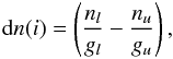(1997) and is defined as $\begin{array}{ccc}\mathrm{d}\mathit{n}\mathrm{\left(}\mathit{i}\mathrm{\right)}\mathrm{=}\left(\frac{{\mathit{n}}_{\mathit{l}}}{{\mathit{g}}_{\mathit{l}}}\mathrm{-}\frac{{\mathit{n}}_{\mathit{u}}}{{\mathit{g}}_{\mathit{u}}}\right)\mathit{,}& & \end{array}$(21)where the indexes u and l stand for the upper and lower level of transition i. In Eq. (20), the gas temperature T_i and turbulence velocity σ_i are indexed according to the line, since in the comparison we only retain the physical parameters that lead to the maximum opacity for this particular line. The opacity ratio thus correlates to the population density ratio considered by Yates et al. (1997) through $\begin{array}{ccc}\frac{{\mathit{\tau }}_{\mathrm{1}}}{{\mathit{\tau }}_{\mathrm{2}}}& \mathrm{=}& \\ & & \mathrm{\times }\hspace{0.17em}{\left[\frac{\mathrm{2}{\mathit{k}}_{\mathrm{B}}{\mathit{T}}_{\mathrm{1}}}{\mathit{m}}\mathrm{+}{\mathit{\sigma }}_{\mathrm{1}}^{\mathrm{2}}\right]}^{\mathrm{-}\frac{\mathrm{1}}{\mathrm{2}}}{\left[\frac{\mathrm{2}{\mathit{k}}_{\mathrm{B}}{\mathit{T}}_{\mathrm{2}}}{\mathit{m}}\mathrm{+}{\mathit{\sigma }}_{\mathrm{2}}^{\mathrm{2}}\right]}^{\frac{\mathrm{1}}{\mathrm{2}}}\mathrm{·}\end{array}$(22)Since the temperatures and turbulence of the models for which the ratios are given in Table 2 of Yates et al. (1997) are unknown, we assume T₁ = T₂ and σ₁ = σ₂ while performing the conversion. Given that the 22 GHz has its maximum inversion at 600 K, as stated in Yates et al. (1997), the maximum error introduced by this assumption is typically of a factor of about two or three. By considering Col. 5 of Table 3, it can be seen that the values currently obtained and the one obtained by Yates et al. (1997) can differ by factors larger than two or three. The differences might arise from the use of plane-parallel geometry in Yates et al. (1997) against spherical geometry in the current work, or because we do not consider the effect introduced by the dust photon pumping in the current study. By examining the results of the comparison reported for o–H₂O in Table 3 and for the lines with frequencies higher than 1.3 THz (λ < 230 μm), we can see that the ratios can take high values above this threshold frequency and tend to increase while the frequency increases. Since this behaviour is correlated with the shape of the dust emission, it can be guessed that a quantitative comparison between the two works is plagued by the absence of consideration of dust radiation in the present work.

Comparing to previous calculations (Neufeld & Melnick 1991; Yates et al. 1997), we find that the 8_5,4 − 7_6,1 (1165 GHz), 7_4,4 − 6_5,1 (1173 GHz), and 8_5,3 − 7_6,2 (1191 GHz) lines can show population inversion with substantial opacities, regardless of the set of rate coefficients used. These lines were not predicted to be masers in the previous studies. The rest of the lines considered in this work agree with the predictions of Yates et al. (1997) with respect to the possibility of masing action, at least for the lines that show substantial inversion.

Considering the effects introduced by the collisional rate coefficients, we find that the variations from one set to another are moderate. The lines which are found to be inverted are the same, regardless of the set considered, and most of the opacities show variations of the order of a factor two or less. Our method of treating the RT of the maser lines introduces large differences in the computed line opacities; indeed, for most of the lines, the opacities derived with the exact treatment are lower by up to a factor four to five in comparison to the opacities derived with the approximated treatment.

Interestingly, we find that many lines can show substantial inversion. This is in agreement with the observations made by Menten et al. (2008) who report the fluxes of nine maser transitions of water. Note that the 437 GHz 7_5,3 − 6_6,0, whose first detection is reported in the latter study, is expected to show a substantial inversion (as was found in Yates et al. 1997) while this line was not found to be inverted by Neufeld & Melnick (1991).

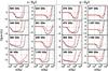Fig. 9 Opacity as a function of H2 volume density for various o–H2O and p–H2O lines which are found to be substantially inverted at TK = 500 K (red lines) and TK = 1000 K (black lines).

Finally, Humphreys et al. (2001) presented models for the excitation of the 22, 183, 321, and 325 GHz water lines in the circumstellar envelopes (CSE) of AGB stars. They found the different masing lines to be excited in specific regions of the CSE, thus predicting different morphologies of the emission maps for the masing lines they considered. A direct comparison with their results is not possible, since in their study the model that describes the circumstellar envelope is rather complex. They first compute the H₂ volume density, gas temperature, and expansion velocity from a hydrodynamical code. As a second step, they randomly define masing spots in the envelope and solve the 1D transfer problem for the various spots using the LVG approximation. The physical parameters that concern each emitting spot is defined according to its distance to the star with respect to the parameters obtained from the hydrodynamical model. Finally, the level populations derived from the LVG calculation are then used in a code that propagates the radiation and that takes into account maser saturation in order to calculate the emission of each spot. Running a model of this kind is out of the scope of the current study, but it is possible to qualitatively discuss their results with the current ones. In Fig. 9 we show the opacities of various water maser lines as a function of the H₂ volume density. The rate coefficients used consider o–H₂ as a collisional partner and are taken from SET2. The opacities are obtained using the treatment for maser propagation and for each line the opacity is given at 500 K and 1000 K.

One of the conclusions drawn by Humphreys et al. (2001) is that the 321 GHz and 22 GHz lines are sensitive to the acceleration zone of the CSE. Additionally, the 321 GHz line is predicted to trace only a region close to the star while the 22 GHz emission extends farther outside (see Fig. 9 of Humphreys et al. 2001). Considering the opacities currently obtained and reported in Fig. 9, we can see that the current results support those findings. Indeed, at densities ~10⁹ cm^-3, the 22 GHz line is the only masing line which is still subsequently inverted. At such a high H₂ density the other masing lines are found to be collisionaly quenched. Moreover, the 321 GHz line is inverted only at relatively high H₂ densities, i.e. n(H₂) > 2  ×  10⁷ cm^-3, which supports the fact that this line only traces the innermost part of the CSE. Humphreys et al. (2001) also find that the emission in the 325 GHz line resembles that of the 22 GHz. In the current study, by examining the behaviour of the opacities of those two lines shown in Fig. 9, we can indeed see that these lines have similar excitation conditions. Additionaly Humphreys et al. (2001) predicted the 183 GHz line to be inverted in the outermost part of the CSE. In this region, the H₂ density is too low to produce inversion in the other masers. Referring to Fig. 9, we can see that at n(H₂) ~10⁶ cm^-3, the 183 GHz line is indeed subsequently inverted while the other lines are not. Finally, considering the behaviour of the opacities reported in Fig. 9, it is possible to qualitatively predict the morphology that the lines not considered by Humphreys et al. (2001) should have. As an example, the emission in the 380 GHz line should resemble the 183 GHz emission and the 439 GHz and 470 GHz lines should behave in a similar way to the 321 GHz line.

5. Conclusions

The present work deals with obtaining a self-consistent solution for the problem of maser propagation within the scope of non-local radiative transfer. Test cases are presented for the water molecule in which the importance of dealing with maser propagation is emphasised, by comparison to a simplified treatment for the radiative transfer. The main conclusions are:

• 1.

  A self-consistent solution for the radiative transfer in masing lines can be obtained within the scope of the short characteristic method, with subsequent modification of the algorithm used to treat thermal lines due to the integro-differential nature of the transfer equation.

• 2.

  The preconditioning of the statistical equilibrium equations is not feasible using the current method nor can the Ng acceleration technique be used, so that the algorithm has the convergence rate of the Lambda iterative scheme.

• 3.

  The test cases performed for the water molecule have shown that neglecting maser propagation can lead to substantial errors in the estimate of the masing-line opacities, with differences greater than a factor of two. Dealing with strongly inverted masers means errors of several orders of magnitude in the prediction of line intensities.

• 4.

  In the region where strong masing lines are present, the radiation field in these lines perturbs the whole population of the molecule. Therefore, including maser propagation also modifies the determination of line opacities for purely thermal lines and in the present test cases, maximum differences of the order of 10 to 20 percent are found between the two methods adopted. Nevertheless, the number of lines affected is rather low and most of the lines have identical optical depths in the two treatments. Given the larger computational time required to solve the maser propagation, the approximation used in this study is a good alternative if one is concerned with interpreting the emission of non-masing lines.

• 5.

  We give predictions of H₂O maser opacities for physical conditions typical of circumstellar envelopes of AGB stars. In addition, the predictions based on various sets of rate coefficients involving He, p–H₂, or o–H₂ are compared. We find that from one set to another, the relative opacities of the masing lines are similar. However, the absolute scale of the opacities are within a factor ~2 depending on the set used.

Acknowledgments

The authors want to thank the referee M.D. Gray for the useful comments that enabled us to improve the current manuscript. We also want to thank A. Baudry for useful discussions concerning the current study. The authors want to thank J. Roberts and T. Bell for their careful reading of the manuscript. This paper was partially supported within the programme CONSOLIDER INGENIO 2010, under grant Molecular Astrophysics: The Herschel and ALMA Era.- ASTROMOL (Ref.: CSD2009- 00038). We also thank the Spanish MICINN for funding support through grants AYA2006-14876 and AYA2009-07304.

References

All Tables

All Figures

	Fig. 1 Variation of the averaged radiation field (solid line) as a function of the initial radiation field entering in the determination of the absorption coefficient. The dashed line corresponds to a straight line of slope unity. The solution of the problem corresponds to the intersection between the two curves. The squares correspond to the averaged radiation field obtained at each iteration.
In the text

	Fig. 2 Schematic diagram showing the availability of incoming intensities during the inward propagation.
In the text

Fig. 3 Isocontours of the o–H2O opacities at line centre for the 616 − 523 line at 22 GHz, the 414 − 321 line at 380 GHz, and the 423 − 330 line at 448 GHz. The left column corresponds to the models where the treatment of maser propagation is omitted and the right column to the current results (see text). The isocontour values and the correspondence between grey scale and opacity values are displayed at the top of the two columns. The isocontours that correspond to opacities of − 4 and − 40 are displayed in thick blue lines. Negative values for the opacity correspond to red lines.

In the text

Fig. 4 Comparison between the opacities derived with (solid lines) or without (dashed lines) accounting for maser propagation for the masers at 22 GHz, 380 GHz, and 448 GHz. The left column corresponds to a cut in density at n(H2) = 2    ×    107 cm-3; the differences are shown with respect to variations in X(H2O). The right column corresponds to a fixed water abundance, i.e. X(H2O) = 4    ×    10-4.

In the text

	Fig. 5 Brightness temperatures for the 22 GHz line obtained with the exact treatment (solid lines) and with the approximated treatment (dashed lines). The intensities correspond to a line of sight that crosses the centre of the sphere and are given for the rest frequency of the line.
In the text

	Fig. 6 Emerging brightness temperature of the 22 GHz line for the model with n(H2) = 4    ×    107 and X(H2O) = 6    ×    10-4. The solid line corresponds to the intensity predicted by the exact calculation, the dashed line to the intensity predicted by the approximated RT (see text).
In the text

	Fig. 7 Ratio as a function of the offset to line centre and of the normalized radius in the cloud. This ratio is given for the 22 GHz line and corresponds to the model with n(H2) = 4    ×    107 and X(H2O) = 6 × 10-4. The two plots correspond to a) the exact treatment and b) an approximated treatment (see text).
In the text

	Fig. 8 The left column corresponds to the opacity of three purely thermal lines obtained in a treatment where masing lines are treated explicitly. The right column corresponds to the ratio rτ = τoff/τon of the opacities obtained with the two treatments (see text).
In the text

	Fig. 9 Opacity as a function of H2 volume density for various o–H2O and p–H2O lines which are found to be substantially inverted at TK = 500 K (red lines) and TK = 1000 K (black lines).
In the text

References

- Anderson, N., & Watson, W. D. 1993, ApJ, 407, 620 [NASA ADS] [CrossRef] [Google Scholar]
- Bettwieser, E. 1976, A&A, 50, 231 [NASA ADS] [Google Scholar]
- Bettwieser, E. V., & Kegel, W. H. 1974, A&A, 37, 291 [NASA ADS] [Google Scholar]
- Cernicharo, J., Thum, C., Hein, H., et al. 1990, A&A, 231, L15 [NASA ADS] [Google Scholar]
- Cernicharo, J., Gonzalez-Alfonso, E., Alcolea, J., Bachiller, R., & John, D. 1994, ApJ, 432, L59 [NASA ADS] [CrossRef] [Google Scholar]
- Cernicharo, J., González-Alfonso, E., & Bachiller, R. 1996, A&A, 305, 5 [Google Scholar]
- Cernicharo, J., Pardo, E., Serabyn, et al. 1999, ApJ, 520, L131 [NASA ADS] [CrossRef] [Google Scholar]
- Cernicharo, J., Pardo, J. R., & Weiss, A. 2006a, ApJ, 646, L49 [NASA ADS] [CrossRef] [Google Scholar]
- Cernicharo, J., Goicoechea, J., Pardo, J. R., & Asensio-Ramos, A. 2006b, ApJ, 642, 940 [NASA ADS] [CrossRef] [Google Scholar]
- Cheung, A. C., Rank, D. M., Townes, C. H., et al. 1969, Nature, 221, 626 [NASA ADS] [CrossRef] [Google Scholar]
- Collison, A. J., & Nedoluha, G. E. 1995, ApJ, 442, 311 [NASA ADS] [CrossRef] [Google Scholar]
- Daniel, F., & Cernicharo, J. 2008, A&A, 488, 1237 [NASA ADS] [CrossRef] [EDP Sciences] [Google Scholar]
- Daniel, F., Dubernet, M., Pacaud, F., & Grosjean, A. 2010, A&A, 517, A13 [NASA ADS] [CrossRef] [EDP Sciences] [Google Scholar]
- Daniel, F., Dubernet, M., & Grosjean, A. 2011, A&A, 536, A76 [NASA ADS] [CrossRef] [EDP Sciences] [Google Scholar]
- Davies, R. D., Rowson, B., Booth, R. S., et al. 1967, Nature, 213, 1109 [NASA ADS] [CrossRef] [Google Scholar]
- Deguchi, S., & Watson, W. D. 1989, ApJ, 340, L17 [NASA ADS] [CrossRef] [Google Scholar]
- Dubernet, M.-L., Daniel, F., Grosjean, A., et al. 2006, A&A, 460, 323 [NASA ADS] [CrossRef] [EDP Sciences] [Google Scholar]
- Dubernet, M.-L., Daniel, F., Grosjean, A., & Lin, C. Y. 2009, A&A, 497, 911 [NASA ADS] [CrossRef] [EDP Sciences] [Google Scholar]
- Elitzur, M. 1992, Astrophys. Space Sci. Lib., 170 [Google Scholar]
- Elitzur, M. 1994, ApJ, 422, 751 [NASA ADS] [CrossRef] [Google Scholar]
- Elitzur, M., Hollenbach, D. J., & McKee, C. F. 1989, ApJ, 346, 983 [NASA ADS] [CrossRef] [Google Scholar]
- Emmering, R. T., & Watson, W. D. 1994, ApJ, 424, 991 [NASA ADS] [CrossRef] [Google Scholar]
- Faure, A., Crimier, N., Ceccarelli, C., et al. 2007, A&A, 472, 1029 [NASA ADS] [CrossRef] [EDP Sciences] [Google Scholar]
- Fish, V. L. 2007, IAU Symp., 242, 71 [NASA ADS] [Google Scholar]
- González-Alfonso, E., Cernicharo, J., Bachiller, R., & Fuente, A. 1995, A&A, 293, L9 [NASA ADS] [Google Scholar]
- González-Alfonso, E., Cernicharo, J., Alcolea, J., & Orlandi, M. A. 1998, A&A, 334, 1016 [NASA ADS] [Google Scholar]
- Gray, M. 1999, Royal Soc. London Philos. Trans. Ser. A, 357, 3277 [NASA ADS] [CrossRef] [Google Scholar]
- Green, S., Maluendes, S., & McLean, A. D. 1993, ApJS, 85, 181 [NASA ADS] [CrossRef] [Google Scholar]
- Humphreys, E. M. L. 2007, IAU Symp., 242, 471 [Google Scholar]
- Humphreys, E. M. L., Yates, J. A., Gray, M. D., Field, D., & Bowen, G. H. 2001, A&A, 379, 501 [NASA ADS] [CrossRef] [EDP Sciences] [Google Scholar]
- Kylafis, N. D., & Pavlakis, K. G. 1999, NATO ASIC Proc. 540: The Origin of Stars and Planetary Systems, 553 [Google Scholar]
- Menten, K., & Melnick, G. J. 1991, ApJ, 377, 647 [NASA ADS] [CrossRef] [Google Scholar]
- Menten, K. L., Melnick, G. J., & Phillips, T. G. 1990a, ApJ, 350, L41 [NASA ADS] [CrossRef] [Google Scholar]
- Menten, K. L., Melnick, G. J., Phillips, T. G., & Neufeld, D. A. 1990b, ApJ, 363, L27 [NASA ADS] [CrossRef] [Google Scholar]
- Menten, K. M., Lundgren, A., Belloche, A., Thorwirth, S., & Reid, M. J. 2008, A&A, 477, 185 [NASA ADS] [CrossRef] [EDP Sciences] [Google Scholar]
- Neufeld, D. A. 1992, ApJ, 393, L37 [NASA ADS] [CrossRef] [Google Scholar]
- Neufeld, D. A., & Melnick, G. J. 1991, ApJ, 368, 215 [NASA ADS] [CrossRef] [Google Scholar]
- Olson, G. L., & Kunasz, P. B. 1987, J. Quant. Spectr. Rad. Transt., 38, 325 [NASA ADS] [CrossRef] [Google Scholar]
- Phillips, T. G., Kwan, J., & Huggins, P. J. 1980, in Interstellar Molecules, ed. B. H. Andrew (Dordrecht: Reidel), IAU Symp., 87, 21 [NASA ADS] [Google Scholar]
- Rybicki, G. B., & Hummer, D. G. 1991, A&A, 245, 171 [NASA ADS] [Google Scholar]
- Waters, J. W., Gustincic, J. J., Kakar, R. K., et al. 1980, ApJ, 235, 57 [NASA ADS] [CrossRef] [Google Scholar]
- Watson, W. D., Sarma, A. P., & Singleton, M. S. 2002, ApJ, 570, L37 [NASA ADS] [CrossRef] [Google Scholar]
- Weaver, H., Williams, D. R. W., Dieter, N. H., & Lum, W. T. 1965, Nature, 208, 29 [NASA ADS] [CrossRef] [Google Scholar]
- Yates, J. A., Field, D., & Gray, M. D. 1997, MNRAS, 285, 303 [NASA ADS] [Google Scholar]