| Issue |
A&A
Volume 552, April 2013
|
|
|---|---|---|
| Article Number | L2 | |
| Number of page(s) | 6 | |
| Section | Letters | |
| DOI | https://doi.org/10.1051/0004-6361/201321110 | |
| Published online | 13 March 2013 | |
Spatially resolved H2 emission from a very low-mass star⋆,⋆⋆,⋆⋆⋆
1
Max – Planck – Institut für Radioastronomie,
Auf dem Hügel 69,
53121
Bonn,
Germany
e-mail:
This email address is being protected from spambots. You need JavaScript enabled to view it.
2
INAF – Osservatorio Astronomico di Roma via Frascati 33,
00040
Monteporzio Catone,
Italy
Received: 15 January 2013
Accepted: 23 February 2013
Abstract
Context. Molecular outflows from very low-mass stars (VLMSs) and brown dwarfs have been studied very little. So far, only a few CO outflows have been observed, allowing us to map the immediate circumstellar environment.
Aims. We present the first spatially resolved H2 emission around IRS54 (YLW 52), a ~0.1–0.2 M⊙ Class I source.
Methods. By means of VLT SINFONI K-band observations, we probed the H2 emission down to the first ~50 AU from the source.
Results. The molecular emission shows a complex structure delineating a large outflow cavity and an asymmetric molecular jet. Thanks to the detection of several H2 transitions, we are able to estimate average values along the jet-like structure (from source position to knot D) of AV ~ 28 mag, T ~ 2000−3000 K, and H2 column density N(H2) ~ 1.7 × 1017 cm-2. This allows us to estimate a mass loss rate of ~2 × 10⁻¹⁰ M⊙ yr-1 for the warm H2 component. In addition, from the total flux of the Br γ line, we infer an accretion luminosity and mass accretion rate of 0.64 L⊙ and ~3 × 10⁻⁷M⊙ yr-1, respectively. The outflow structure is similar to those found in low-mass Class I and CTTS. However, the Lacc/Lbol ratio is very high (~80%), and the mass accretion rate is about one order of magnitude higher when compared to objects of roughly the same mass, pointing to the young nature of the investigated source.
Key words: stars: formation / circumstellar matter / stars: winds, outflows / ISM: jets and outflows / infrared: ISM
Based on observations collected at the European Southern Observatory Paranal, Chile (ESO programme 385.C-0893(A)).
Appendices are available in electronic form at http://www.aanda.org
The reduced datacube is only available at the CDS via anonymous ftp to cdsarc.u-strasbg.fr(130.79.128.5) or via http://cdsarc.u-strasbg.fr/viz-bin/qcat?J/A+A/552/L2
© ESO, 2013
1. Introduction
Protostellar jets and outflows are associated with the first stages of stellar evolution. They are usually found in active young stellar objects (YSOs), in which a significant fraction of the circumstellar material is still accreting onto the protostar. Jets and outflows can therefore be considered an outcome of the accretion activity. During the early evolutionary phase, outflows are usually traced through molecular emission lines. Molecular outflows from low- and high-mass protostars have been extensively studied through observations of CO lines (Bachiller & Tafalla 1999; Arce et al. 2007). These observations have revealed many common observational characteristics between both mass regimes, which points to a common outflow mechanism working from low- to high-mass protostars (Arce et al. 2007).
Molecular outflows from very low-mass stars (VLMSs) and brown-dwarfs (BDs) have been studied very little, especially during their early evolutionary phase. Only recently have CO submillimetre observations been able to provide direct imaging of a small number of molecular outflows from VLMSs (Phan-Bao et al. 2008, 2011). Most of the few observations of jets from BDs and VLMSs, however, involve relatively evolved, classical T Tauri-like YSOs, mainly studied through detecting forbidden emission lines (FELs) (Fernández & Comerón 2001; Whelan et al. 2012) in their spectra, and/or spectro-astrometry of FELs (Whelan et al. 2005, and ref. therein). So far, no observation of resolved molecular hydrogen emission line (MHEL) regions has existed for VLMSs or BDs. The presence of MHEL regions are typical of the spectrum of low-mass Class I sources (Davis et al. 2001; Garcia Lopez et al. 2008; Davis et al. 2011), and they are usually associated with an FEL region. Thus, one should also expect MHEL regions around young BDs and VLMSs.
In this context, we present here the first H2 1-0S(1) spectro-imaging of an outflow from a Class I VLMS, IRS54 (YLW 52). This source (α = 16:27:51.7, δ = −24:31:46.0) is located outside of the main clouds in the Ophiuchus star-forming region, and it has been classified as a late-stage Class I source with a bolometric luminosity of ~0.78 L⊙ (van Kempen et al. 2009). IRS54 is thus in its main accretion phase, representing one of the lowest luminosity sources for which an H2 outflow has been spatially resolved.
2. Observations and data analysis
The data were acquired on 14 June 2010 at the Very Large Telescope at Paranal Observatory, Chile, using the integral field spectrograph SINFONI at medium resolution in the K-band (R ~ 4000). The chosen pixel scale was 100 mas, corresponding to a 3′′ × 3′′ field of view. The observations were acquired under 0 4 seeing (DIMM FWHM), leading to a spatial resolution of 48 AU at the location of IRS54 (d ~ 120 pc). The total integration time is 1200 s. To correct for atmospheric response, observations of a telluric standard star of spectral type B were performed. The main data reduction process was done using the SINFONI data-reduction pipeline, i.e., dark and bad pixel masks, flat-field corrections, optical distortion correction, and wavelength calibration using arc lamps. To test the goodness of the wavelength calibration, we applied the final wavelength transformation matrix to a sky cube. By measuring the wavelength of the OH lines present in the cube, we found a systematic wavelength shift of ~2.2 Å with respect to their theoretical value. The final data cube was thus shifted in wavelength to take this error into account. In addition to the SINFONI pipeline, the STARLINK software was used to correct the spectrum from atmospheric absorption and to flux-calibrate the data. With this aim, the standard star spectrum was extracted by collapsing the central region of the data cube. The Brγ line was then removed from the standard spectrum before dividing it by a normalised blackbody at the appropriate temperature. Then, the spectrum was grown up into a 60 × 70 pixel cube, as was that of our SINFONI data, to correct for the telluric features and to flux-calibrate the data.
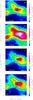 |
Fig. 1 Continuum-subtracted H2 1-0S(1) images of IRS54. Panels a) and c): average over two spectral channels at − 64 km s-1 and –30 km s-1 (panel a)), and +40 km s-1 and +75 km s-1 (panel c)). Panel b): single spectral channel at +6 km s-1. The velocities are corrected from an average cloud velocity of 3.5 km s-1 (Wouterloot et al. 2005; André et al. 2007). Panel d): average H2 1-0S(1) emission over the previous velocity channels. Overplotted are the locations of six spatial regions where spectra were extracted. For reference, contours of the continuum (near the H2 2.122 μm line) down to the FWHM size have been overplotted at the centre of every image (dashed-blue contours). Contours in all panels show values of 1.3, 2.9, 4.5, 5.3, 6.1, 7.7, 9.3 × 10⁻¹⁴ erg s-1 cm-2μm-1. |
The brightest lines present in the K-band SINFONI spectrum are H2 lines from different rovibrational levels and the Br γ line. Because both continuum and line emissions are observed simultaneously, an accurate subtraction of the continuum can be performed, allowing us to obtain very clean images of the different line-emitting regions. To better probe the jet morphology close to the central source, the continuum emission was removed from the IFS cube using the IRAF subroutine “CONTINUUM” iteratively along the dispersion axis at each spatial position of the datacube. All images shown in this letter have been continuum-subtracted using this method. In addition, integral field spectroscopy enables us to obtain precise positional measurements of emission knots relative to each other and to the source continuum. For instance, a ~16 mas positional accuracy can be obtained by taking our seeing conditions and a signal-to-noise ratio of only ~10 into account (position accuracy ~Seeing/(2.35 × SN); Davis et al. 2011).
3. Outflow physics and morphology
Integral field spectroscopic observations allow us to retrieve direct information about the morphology and kinematics of the H2 emission close to the Class I protostar IRS54. Indeed, the H2 2.122 μm line is one of the brightest lines tracing outflow activity in the K-band.
Figure 1 shows the averaged continuum-subtracted H2 1-0S(1) emission across the datacube (panel d), along with the blue- and red-shifted H2 outflow components (panels a and c). In addition, the H2 emission at rest velocity (corresponding to one pixel in the datacube dispersion direction) is shown in panel b. The H2 1-0S(1) spectral image in panel d was contructed by averaging five different velocity channels at the local standard of rest (from − 64 km s-1 to +75 km s-1), while the blue- and red-shifted images correspond to the averaged emission over two pixels in the dispersion direction (–64 km s-1 and –30 km s-1, and at +40 km s-1 and +75 km s-1). The figure shows a very complex H2 morphology with gas displaying an X-shaped spatial distribution superimposed on a more collimated structure, possibly jet-like (see discussion bellow), located westward of IRS54 and extending over ~1′′ (~120 AU). All regions show a knotty structure, with condensations A, B, C, E, and D displaced from the source (Δα, Δδ) at about (13, –04), (04, 05), (03, 04), (–01, 0), and (–03, 0), respectively (see panel d). The overall gas distribution is very similar to the one observed in molecular jets from embedded low-mass protostars, as usually traced by CO/molecular observations (e.g., Tafalla et al. 2004). In this case, however, two well-defined red- and blue-shifted lobes cannot be identified. As shown from the velocity channels represented from panels a to d, red- and blue-shifted emission can be roughly associated with the same spatial regions. It should be noted that the velocities of the channel maps do not correspond to the H2 2.122 μm line peak velocity at any spatial position. Indeed, this line shows a very broad profile with a full width zero intensity of ~200 km s-1, but with a peak velocity of ~0 km s-1 (see Fig. 2). This may suggest that the outflow lies very close to the plane of the sky.
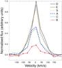 |
Fig. 2 Line profile of the H2 2.122 μm line extracted for six different spatial positions (see Fig. 1 and Table 1 for information about the spatial distribution of the different extracted areas). All line profiles are normalised to the flux of knot D. |
In addition, thanks to detecting several H2 lines, excitation diagrams could be constructed to derive the temperature, H2 column density, and extinction of the molecular gas (e.g., Caratti o Garatti et al. 2006; Garcia Lopez et al. 2010). The results are shown in Table 1. The H2 line fluxes (see Table A.1) were measured at each of the positions indicated in Fig. 1 by simulating “long-slit” spectra with a fixed slit width corresponding to an extraction aperture of 3 × 3 pixels. Temperature and N(H2) values range from ~1840 K to 3340 K and from 2.4 to 20 × 1016 cm-2. The visual extinction, temperature, and N(H2) are higher westward of IRS54, increasing along the jet-like structure towards the source position (knot D and on source), which suggests that the western lobe is the red-shifted lobe of the outflow and that the X-shaped and jet-like structures have different physical conditions. The extinction values found towards the source are very similar to those reported in previous works, where AV values ≳25 mag are reported (Haisch et al. 2004).
Finally, we note that the Br γ emission is not spatially resolved, and it matches the stellar continuum.
4. Accretion and ejection properties
From our observations, it is also possible to derive the accretion luminosity and the mass accretion and ejection rates of IRS54. Using the relation between the luminosity of the Br γ line (L(Br γ)) and the accretion luminosity (Lacc) derived by Calvet et al. (2004), we found an accretion luminosity of Lacc ~ 0.64 L⊙. The luminosity of the Br γ line was measured from the integrated flux across the Br γ line in our cube (F = 4.08 × 10⁻¹⁴ erg s-1 cm-2) and corrected by a visual extinction of 30 mag. Considering the modest bolometric luminosity of this source (Lbol ~ 0.78 L⊙; van Kempen et al. 2009), the accretion luminosity is very high, with an Lacc/Lbol value of ~80%, which is consistent with a very young and active YSO. This supports the idea that IRS54 is a young YSO (van Kempen et al. 2009) still accreting large amounts of circumstellar matter. Assuming Lbol = Lacc+L∗, we find a stellar luminosity of L∗ ~ 0.14 L⊙. We derive a stellar mass and radius of 0.1–0.2 M⊙ and ~2 R⊙ by placing the stellar luminosity into an HR diagram and considering the bithline locus using the evolutionary tracks of Siess et al. (2000) and Stahler (1988). This indicates that IRS54 has spectral type M and is a very low-mass star.
A mass accretion rate of ~3.0 × 10⁻⁷ M⊙ yr-1 is inferred from the observed Lacc, following the expression Ṁacc = (Lacc R∗/G M∗) × (1 − R∗/Ri), Ri being the inner radius of the accretion disk (with Ri = 5 R∗, see Gullbring et al. 1998). The derived value is higher than those found in more evolved objects of roughly the same mass (Natta et al. 2006; Gatti et al. 2006), again pointing to the young nature of this source.
H2 diagnostics.
The mass-loss rate carried by the warm molecular component (ṀH2) can be computed from the derived N(H2) values using the expression ṀH2 = 2 μ mH N(H2) A dvt/dlt (see, e.g., Davis et al. 2001, 2011). Here, A is the area of the emitting region, μ is the mean atomic weight, and dlt and dvt are the projected length and the tangential velocity. We have assumed that the area where the molecular hydrogen is emitted is equal to the extent of the flow along the jet axis from position S to D (~05) multiplied by the width of the flow (i.e. the seeing). We have considered an average N(H2) value for this region of ~1.7 × 1017 cm-2. To retrieve vt, the inclination angle of the outflow with respect to the line of sight should be known. As outlined before, the radial velocities suggest that the outflow is almost in the plane of the sky, and thus, an estimate of the jet velocity from an unknown flow angle is too uncertain. Therefore, we assume the width of the H2 lines presented in Fig. 2 as a lower limit to the jet velocity, i.e. ~200 km s-1. This gives a value of ṀH2 ≳ 1.6 × 10⁻¹⁰ M⊙ yr-1 which is about two orders of magnitude lower than expected if compared with the derived Ṁacc value (Ṁout/Ṁacc ~ 0.1). The computed ṀH2 value is also around two to three orders of magnitude lower than the ṀH2 value derived for low-mass Class I sources using the same technique (Davis et al. 2011). However, it is worth noting that these sources are likely to be more massive than ours. This suggests that (1) most of the outflow material is transported by a cooler and denser component than traced by the near-IR H2 lines, such as the H2 pure rotational lines (Caratti o Garatti et al. 2008); or (2) most of the H2 has been dissociated, and the jet is mainly atomic. The latter has been observed in other Class I jets, where the measured ṀH2 is around one order of magnitude lower than measured from the [Fe ii] emission (Davis et al. 2011; Nisini et al. 2005).
5. Discussion
Molecular outflows, H2 jets in particular, have been observed from Class 0 to Class II sources through a wide range of masses. Here, we show that MHEL regions are also common in the first evolutionary stages of VLMSs, suggesting that the same launching mechanism is acting from very low- to high-mass stars and across a wide range of evolutionary stages.
In general, MHEL properties are consistent with shock-heated gas from the inner regions of Herbig-Haro objects or from spatially extended wide-angle winds (Davis et al. 2001; Caratti o Garatti et al. 2006; Beck et al. 2008; Davis et al. 2011). The reported gas temperatures and excitation properties of IRS54 are consistent with shock-heated material, as well. Similar values have also been found in low-mass Class I sources and CTTSs (Beck et al. 2008; Davis et al. 2011). The overall outflow structure can be interpreted as the sum of H2 emission excited along a wide-angle cavity, plus the contribution from a jet-like structure. This latter structure is, however, only observed in one of the lobes. This probably indicates different excitation conditions for the two lobes of the jet, i.e. an asymmetric jet in which the blue-shifted lobe might have a higher velocity, dissociating the molecular H2 component. If this is the case, ionic/atomic emission should be present in the eastern jet. Velocity asymmetries have been observed before in other protostellar jets, such as RW Aur (e.g., Melnikov et al. 2009).
IRS 54 is known to possess a large-scale S-shaped bipolar jet as traced by a chain of H2 knots1 extending over several arcminutes (feature f08-01 in Khanzadyan et al. 2004). From wide-field H2 images, the jet appears to precess with a position angle (PA) changing from ~72° in the outermost knots passing through ~78° in the middle part of the jet down to 90° closest to the source (MHO 2129; see also Fig. B.1 in Jørgensen et al. 2009). The strong jet precession may then be at the origin of the outflow cavity, suggesting that the low-velocity H2 emission is gas excited along the cavity walls by the interaction of a wide-angle wind with the ambient material. On the other hand, the PA of the internal jet-like structure detected in our H2 spectral images is consistent with the PA of the innermost knots of the large-scale H2 jet (i.e., MHO 2129). This may support the idea that the denser and more reddened jet-like structure in our images is indeed the upstream region of the H2 jet observed in the wide-field images. Jet precession alone can, however, hardly account for all the observed features shown in Fig. 1. By assuming a lower limit to the jet velocity of ~200 km s-1, the dynamical age of condensations A, B, C, D, and E are around 3.9, 1.9, 1.4, 0.9, and 0.3 yr. This would lead to a precession period of about four years in order to generate the structures (A, B, and C) at each side of the so-called cavity (opening angle ~65°). This period is too short when compared with typical jet fast precession periods (Rosen & Smith 2004; Caratti o Garatti et al. 2008), and not consistent with the longer period suggested by the large-scale jet images (see f08-01 field in Khanzadyan et al. 2004).
On the other hand, a wide-angled wind might be able to explain both the broad line profiles presented in Fig. 2 and the observed features in Fig. 1. Considering the jet-like structure alone (condensations E and D), we have measured the H2 jet width as a function of the distance from the source (see, Fig. B.1). We estimate a full opening angle of the flow of ~23°, fitting a straight line to the points from 40 to 140 AU in Fig. B.1 (see Davis et al. 2011, for more details). Similar values are also found in jets from low-mass Class I sources and CTTSs, which show opening angles between 20° and 42° (Hartigan et al. 2004; Davis et al. 2011). Beyond ≳50 AU, the jet width slowly increases with distance (see Fig. B.1 and Hartigan et al. 2004; Davis et al. 2011) as expected for a free lateral expansion of a supersonic jet (Cabrit 2007). Therefore, the jet collimation must take place within the first ≲50 AU from the source, in agreement with MHD wind models (Dougados et al. 2004). Panoglou et al. (2012) show that molecular hydrogen can survive along MHD disk-wind streamlines. The presence of H2 emission detected at only ~48 AU from the source, together with the broad line profiles shown in Fig. 2, tend to favour the presence of an MHD disk-wind model. Nevertheless, a wide-angled wind alone cannot account for the precessing jet observed in the large-scale images. Therefore, a combination of both a wide-angled wind and a precessing jet is possibly the main mechanism behind the complex H2 structure in IRS54 (Fig. B.2).
6. Conclusions
In this letter, we present the first spatially resolved H2 emission (MHEL) region around IRS54, a Class I VLMS. The H2 emission was detected down to the first ~50 AU from the source, and it shows a very complex morphology. The emission
might be interpreted as coming from the interaction of a wide-angle wind with an outflow cavity and a molecular jet. In addition, the detection of several H2 line transitions and the Br γ line allows us to derive various accretion/ejection properties:
-
We computed the extinction, H2 column den-sity, and temperature values at different outflow spatial posi-tions from the analysis of excitation diagrams. The highestvalues are found westward of IRS54, increasing along the jet-like structure towards the source position. Average values ofAv ~ 28 mag, T = 2000–3000 K, and N(H2) ~ 1.7 × 1017 cm-2 are found along the jet-like structure (knots D and S).
-
We inferred an accretion luminosity and mass accretion rate of 0.64 L⊙ and 3 × 10⁻⁷ M⊙ yr-1 from the total flux of the Br γ emission. From the computed Lacc and the Lbol value found in literature, we derived L∗ ~ 0.14 L⊙, which yields a stellar mass of ~0.1–0.2 M⊙.The accretion luminosity accounts for ~80% of the total luminosity. This, together with the high Ṁacc value, points to the young nature of IRS54.
Online material
Appendix A: H2 line fluxes and spectra
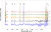 |
Fig. A.1 Continuum-subtracted spectra at five different positions along the outflow (see Fig. 1 and Table A.1). |
H2 line fluxes.
Appendix B: Outflow width and morphology
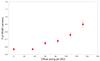 |
Fig. B.1 Width of the H2 1-0S(1) jet-like structure as a function of the distance from the source. The jet width has been estimated by extracting 2-pixel-wide vertical slices to the average H2 spectral image presented in Fig. 1 and fitting a single Gaussian function. Zero offsets correspond to the source positions. |
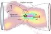 |
Fig. B.2 Sketch showing IRS54 outflow/jet morphology. |
Named MHO 2128-2131, see http://www.astro.ljmu.ac.uk/MHCat/
Acknowledgments
We thank the anonymous referee for the comments that helped improve the paper.
References
- André, P., Belloche, A., Motte, F., & Peretto, N. 2007, A&A, 472, 519 [NASA ADS] [CrossRef] [EDP Sciences] [Google Scholar]
- Arce, H. G., Shepherd, D., Gueth, F., et al. 2007, Protostars and Planets V, 245 [Google Scholar]
- Bachiller, R., & Tafalla, M. 1999, in NATO ASIC Proc. 540: The Origin of Stars and Planetary Systems, eds. C. J. Lada, & N. D. Kylafis, 227 [Google Scholar]
- Beck, T. L., McGregor, P. J., Takami, M., & Pyo, T.-S. 2008, ApJ, 676, 472 [NASA ADS] [CrossRef] [Google Scholar]
- Cabrit, S. 2007, in Lect. Notes Phys. (Berlin: Springer Verlag), eds. J. Ferreira, C. Dougados, & E. Whelan, 723, 21 [Google Scholar]
- Calvet, N., Muzerolle, J., Briceño, C., et al. 2004, AJ, 128, 1294 [NASA ADS] [CrossRef] [Google Scholar]
- Caratti o Garatti, A., Giannini, T., Nisini, B., & Lorenzetti, D. 2006, A&A, 449, 1077 [NASA ADS] [CrossRef] [EDP Sciences] [Google Scholar]
- Caratti o Garatti, A., Froebrich, D., Eislöffel, J., Giannini, T., & Nisini, B. 2008, A&A, 485, 137 [NASA ADS] [CrossRef] [EDP Sciences] [Google Scholar]
- Davis, C. J., Ray, T. P., Desroches, L., & Aspin, C. 2001, MNRAS, 326, 524 [NASA ADS] [CrossRef] [Google Scholar]
- Davis, C. J., Cervantes, B., Nisini, B., et al. 2011, A&A, 528, A3 [NASA ADS] [CrossRef] [EDP Sciences] [Google Scholar]
- Dougados, C., Cabrit, S., Ferreira, J., et al. 2004, Ap&SS, 292, 643 [NASA ADS] [CrossRef] [Google Scholar]
- Fernández, M., & Comerón, F. 2001, A&A, 380, 264 [NASA ADS] [CrossRef] [EDP Sciences] [Google Scholar]
- Garcia Lopez, R., Nisini, B., Giannini, T., et al. 2008, A&A, 487, 1019 [NASA ADS] [CrossRef] [EDP Sciences] [Google Scholar]
- Garcia Lopez, R., Nisini, B., Eislöffel, J., et al. 2010, A&A, 511, A5 [NASA ADS] [CrossRef] [EDP Sciences] [Google Scholar]
- Gatti, T., Testi, L., Natta, A., Randich, S., & Muzerolle, J. 2006, A&A, 460, 547 [NASA ADS] [CrossRef] [EDP Sciences] [Google Scholar]
- Gullbring, E., Hartmann, L., Briceno, C., & Calvet, N. 1998, ApJ, 492, 323 [NASA ADS] [CrossRef] [Google Scholar]
- Haisch, Jr., K. E., Greene, T. P., Barsony, M., & Stahler, S. W. 2004, AJ, 127, 1747 [NASA ADS] [CrossRef] [Google Scholar]
- Hartigan, P., Edwards, S., & Pierson, R. 2004, ApJ, 609, 261 [NASA ADS] [CrossRef] [Google Scholar]
- Jørgensen, J. K., van Dishoeck, E. F., Visser, R., et al. 2009, A&A, 507, 861 [NASA ADS] [CrossRef] [EDP Sciences] [Google Scholar]
- Khanzadyan, T., Gredel, R., Smith, M. D., & Stanke, T. 2004, A&A, 426, 171 [NASA ADS] [CrossRef] [EDP Sciences] [Google Scholar]
- Melnikov, S. Y., Eislöffel, J., Bacciotti, F., Woitas, J., & Ray, T. P. 2009, A&A, 506, 763 [NASA ADS] [CrossRef] [EDP Sciences] [Google Scholar]
- Natta, A., Testi, L., & Randich, S. 2006, A&A, 452, 245 [NASA ADS] [CrossRef] [EDP Sciences] [Google Scholar]
- Nisini, B., Bacciotti, F., Giannini, T., et al. 2005, A&A, 441, 159 (N05) [NASA ADS] [CrossRef] [EDP Sciences] [Google Scholar]
- Panoglou, D., Cabrit, S., Pineau Des Forêts, G., et al. 2012, A&A, 538, A2 [NASA ADS] [CrossRef] [EDP Sciences] [Google Scholar]
- Phan-Bao, N., Riaz, B., Lee, C.-F., et al. 2008, ApJ, 689, L141 [NASA ADS] [CrossRef] [Google Scholar]
- Phan-Bao, N., Lee, C.-F., Ho, P. T. P., & Tang, Y.-W. 2011, ApJ, 735, 14 [NASA ADS] [CrossRef] [Google Scholar]
- Rosen, A., & Smith, M. D. 2004, MNRAS, 347, 1097 [NASA ADS] [CrossRef] [Google Scholar]
- Siess, L., Dufour, E., & Forestini, M. 2000, A&A, 358, 593 [NASA ADS] [Google Scholar]
- Stahler, S. W. 1988, ApJ, 332, 804 [NASA ADS] [CrossRef] [Google Scholar]
- Tafalla, M., Santiago, J., Johnstone, D., & Bachiller, R. 2004, A&A, 423, L21 [NASA ADS] [CrossRef] [EDP Sciences] [Google Scholar]
- van Kempen, T. A., van Dishoeck, E. F., Hogerheijde, M. R., & Güsten, R. 2009, A&A, 508, 259 [Google Scholar]
- Whelan, E. T., Ray, T. P., Bacciotti, F., et al. 2005, Nature, 435, 652 [NASA ADS] [CrossRef] [PubMed] [Google Scholar]
- Whelan, E., Ray, T., Comeron, F., Bacciotti, F., & Kavanagh, P. 2012, ApJ, 761, 120 [NASA ADS] [CrossRef] [Google Scholar]
- Wouterloot, J. G. A., Brand, J., & Henkel, C. 2005, A&A, 430, 549 [NASA ADS] [CrossRef] [EDP Sciences] [Google Scholar]
All Tables
All Figures
|
Fig. 1 Continuum-subtracted H2 1-0S(1) images of IRS54. Panels a) and c): average over two spectral channels at − 64 km s-1 and –30 km s-1 (panel a)), and +40 km s-1 and +75 km s-1 (panel c)). Panel b): single spectral channel at +6 km s-1. The velocities are corrected from an average cloud velocity of 3.5 km s-1 (Wouterloot et al. 2005; André et al. 2007). Panel d): average H2 1-0S(1) emission over the previous velocity channels. Overplotted are the locations of six spatial regions where spectra were extracted. For reference, contours of the continuum (near the H2 2.122 μm line) down to the FWHM size have been overplotted at the centre of every image (dashed-blue contours). Contours in all panels show values of 1.3, 2.9, 4.5, 5.3, 6.1, 7.7, 9.3 × 10⁻¹⁴ erg s-1 cm-2μm-1. |
| In the text | |
|
Fig. 2 Line profile of the H2 2.122 μm line extracted for six different spatial positions (see Fig. 1 and Table 1 for information about the spatial distribution of the different extracted areas). All line profiles are normalised to the flux of knot D. |
| In the text | |
|
Fig. A.1 Continuum-subtracted spectra at five different positions along the outflow (see Fig. 1 and Table A.1). |
| In the text | |
|
Fig. B.1 Width of the H2 1-0S(1) jet-like structure as a function of the distance from the source. The jet width has been estimated by extracting 2-pixel-wide vertical slices to the average H2 spectral image presented in Fig. 1 and fitting a single Gaussian function. Zero offsets correspond to the source positions. |
| In the text | |
|
Fig. B.2 Sketch showing IRS54 outflow/jet morphology. |
| In the text | |
Current usage metrics show cumulative count of Article Views (full-text article views including HTML views, PDF and ePub downloads, according to the available data) and Abstracts Views on Vision4Press platform.
Data correspond to usage on the plateform after 2015. The current usage metrics is available 48-96 hours after online publication and is updated daily on week days.
Initial download of the metrics may take a while.