| Issue |
A&A
Volume 552, April 2013
|
|
|---|---|---|
| Article Number | A13 | |
| Number of page(s) | 13 | |
| Section | Stellar atmospheres | |
| DOI | https://doi.org/10.1051/0004-6361/201220813 | |
| Published online | 13 March 2013 | |
Pure-hydrogen 3D model atmospheres of cool white dwarfs
1 Zentrum für Astronomie der Universität Heidelberg, Landessternwarte, Königstuhl 12, 69117 Heidelberg, Germany
e-mail: This email address is being protected from spambots. You need JavaScript enabled to view it.
; This email address is being protected from spambots. You need JavaScript enabled to view it.
2 Leibniz-Institut für Astrophysik Potsdam, An der Sternwarte 16, 14482 Potsdam, Germany
e-mail: This email address is being protected from spambots. You need JavaScript enabled to view it.
3 Centre de Recherche Astrophysique de Lyon, UMR 5574: CNRS, Université de Lyon, École Normale Supérieure de Lyon, 46 allée d’Italie, 69364 Lyon Cedex 07, France
e-mail: This email address is being protected from spambots. You need JavaScript enabled to view it.
Received: 28 November 2012
Accepted: 7 February 2013
Abstract
A sequence of pure-hydrogen CO5BOLD 3D model atmospheres of DA white dwarfs is presented for a surface gravity of log g = 8 and effective temperatures from 6000 to 13 000 K. We show that convective properties, such as flow velocities, characteristic granulation size and intensity contrast of the granulation patterns, change significantly over this range. We demonstrate that these 3D simulations are not sensitive to numerical parameters unlike the 1D structures that considerably depend on the mixing-length parameters. We conclude that 3D spectra can be used directly in the spectroscopic analyses of DA white dwarfs. We confirm the result of an earlier preliminary study that 3D model spectra provide a much better characterization of the mass distribution of white dwarfs and that shortcomings of the 1D mixing-length theory are responsible for the spurious high-log g determinations of cool white dwarfs. In particular, the 1D theory is unable to account for the cooling effect of the convective overshoot in the upper atmospheres.
Key words: convection / line: profiles / stars: atmospheres / white dwarfs / hydrodynamics
© ESO, 2013
1. Introduction
The multidimensional radiation-hydrodynamics (RHD) treatment of convective motions in hydrogen-atmosphere DA white dwarfs was pioneered by the Kiel group some fifteen years ago (Ludwig et al. 1994; Steffen et al. 1995; Freytag et al. 1996). These studies have revealed that the differences between spectra computed on the basis of 2D RHD simulations and those computed from standard 1D hydrostatic models were small. However, recent research developments make it advisable to pursue the computation of RHD models. First of all, three-dimensional RHD computations (hereafter 3D simulations) became accurate enough to be the reference in quantitative spectroscopy, in particular for the abundance determinations in the Sun (Asplund et al. 2009; Caffau et al. 2011). Secondly, the spectroscopic technique in DA white dwarfs, which consists in comparing the observed line profiles of the Balmer series with the predictions of detailed model atmospheres (Weidemann & Koester 1980; Bergeron et al. 1992a), became more widely used, with larger samples (Eisenstein et al. 2006) and higher signal-to-noise ratio (S/N) observations (Gianninas et al. 2011). For high quality observations (S/N > 50), it is often quoted that the relative uncertainties in the atmospheric parameters, the effective temperature (Teff) and surface gravity (log g, in cgs units), are of the order of 1% (Liebert et al. 2005; Koester et al. 2009b). As a consequence, white dwarfs have been used as spectroscopic standards to achieve high-precision calibrations at the 1% level (see, e.g., Bohlin 2000).
It has been shown long ago that the spectroscopically determined masses of cool DA white dwarfs (Teff < 13 000 K) were as much as 20% higher than those of hotter DA white dwarfs (Bergeron et al. 1990, 1992a). This discrepancy is now observed in the spectroscopic mass distribution of all surveys of DA white dwarfs (Tremblay et al. 2011a; Gianninas et al. 2011). Multiple attempts were made to explain this behaviour (Koester et al. 2009a; Tremblay et al. 2010) but were unsuccessful. However, it was suggested that because convection becomes significant in the photosphere almost exactly as the so-called high-log g problem becomes apparent, the 1D mixing-length theory (MLT; Böhm-Vitense 1958) was likely the culprit. Therefore, Tremblay et al. (2011b, hereafter Paper I) computed the first four non-grey 3D model atmospheres of DA white dwarfs (12 800 > Teff (K) > 11 300 and log g = 8) using the CO5BOLD RHD code (Freytag et al. 2012). The code is usually applied to stars with deep convective envelopes where it is not possible for the simulation domain to span the full convection zone. However, the convection zone in these hot white dwarfs is in fact thinner than the simulation domain in the vertical direction.
The aim of Paper I was to predict quantitatively how the atmospheric parameters are changed by using 3D spectra instead of the standard 1D spectra. As a consequence, the methodological approach was to do a differential analysis, by comparing both the spectra computed from 3D structures, and 1D hydrostatic (LHD) structures (Caffau & Ludwig 2007) relying the same microphysics and opacity bins as the 3D simulations, with standard 1D spectra of white dwarfs (Tremblay et al. 2011a). It was found that the 3D log g corrections had the correct amplitude to solve the high-log g problem for DA white dwarfs in the range of Teff studied in the paper. It was concluded that a weakness in the 1D MLT theory was creating the high-log g problem.
Several aspects of the 3D calculations can be improved in order to understand to which extend these simulations can solve the high-log g problem, and ultimately, to use them in the spectroscopic analyses of white dwarfs. First of all, it is desirable to compute cooler 3D simulations, since the high-log g problem is most prominent around Teff = 10 000 K (see, e.g., Fig. 1 of Paper I). Furthermore, it is necessary to have 3D simulations containing realistic microphysical properties in order to compare them directly to white dwarf observations. For instance, the four 3D simulations computed in Paper I rely on an equation-of-state (EOS) and opacity table (including an opacity binning procedure) that have different microphysics in comparison to standard 1D model atmospheres.
We tackle these shortcomings in this work by producing an improved sequence of 12 DA model atmospheres, covering the range 13 000 > Teff (K) > 6000 at log g = 8. In Sect. 2, we discuss about the precision of our 3D simulations. In Sect. 3, we present the properties of our sequence of 3D computations. Model spectra are computed in Sect. 4 and improved 3D log g corrections are derived in relation to the high-log g problem. The conclusion follows in Sect. 5.
2. Establishing absolute properties
The main objective of our study is to produce 3D model atmospheres that represent real stellar conditions as closely as possible with the aim of performing direct comparisons of these models with observations. We must beforehand understand the sources of the differences between these 3D structures and standard 1D structures, both computed with established well-known codes. In other words, we must carefully compare the codes producing these model atmospheres. Several groups have in the past computed grids of 1D model atmospheres for DA white dwarfs (e.g., Bergeron et al. 1992a; Finley et al. 1997; Kowalski & Saumon 2006). Recent theoretical developments include the improved modelling of the Lyman quasi-molecular satellites (Allard et al. 2004), the calculation of the Ly-α red wing opacity due to H2-H collisions (Kowalski & Saumon 2006) and the publication of new Stark broadening profiles (Tremblay & Bergeron 2009) including in a consistent way the non-ideal gas effects of Hummer & Mihalas (1988). All of these improvements are now included in our 1D model atmosphere code described in Tremblay et al. (2011a) and references therein. We note that the D. Koester model atmosphere code includes very similar physics at the time of publication (see, e.g., Girven et al. 2011). Hence, while we specifically use the Tremblay et al. (2011a) grid in this work, it is appropriate to describe them from now on as standard 1D models.
The treatment of convection is obviously a genuine difference between the 3D CO5BOLD code and the standard 1D codes. As a consequence, it is difficult to isolate other possible differences between both codes. This hurdle is removed by using the 1D LHD code, in which microphysics and radiative transfer numerical schemes (e.g., the opacity binning) are identical to those included in the 3D simulations. In Fig. 1, we compare our latest 1D LHD structures and standard 1D structures, which shows that we were successful in explaining and eliminating as much as possible the differences between both codes. Our improvements made to the LHD code are described in this section.
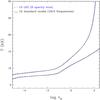 |
Fig. 1 Atmospheric temperature as a function of the logarithm of the Rosseland optical depth for DA models with effective temperatures of 8000 (bottom) and 12 000 K (top). We show the standard 1D structures (solid black line) from Tremblay et al. (2011a), recomputed with a slightly higher numerical precision, and the improved 1D LHD structures (dashed blue line) described in the text. |
2.1. Input microphysics
In Paper I, the CO5BOLD and LHD structures were based on different microphysics (Ludwig et al. 1994) in comparison to the one used in prevalent 1D white dwarf codes. The former codes rely on pre-computed EOS and opacity tables as input, and it is fairly straightforward to replace these tables with ones that are computed with the same microphysics as in standard 1D models. This is the first step of our improvement of the LHD structures. We found that the non-ideal EOS typically used in white dwarfs has a negligible effect on the predicted structures (for Teff > 6000 K and log τR < 3) compared to the ideal EOS utilised in Paper I. In the case of the improved opacities, the effect is mild, and it is shown in Sect. 4.3 that the corresponding log g correction is of the order of 0.03 dex.
We now look at the opacity binning approach, which is a known difference between the LHD and standard white dwarf codes. In Paper I, we used 7 band-averaged opacities to describe the band-integrated radiative transfer, based on the procedure laid out in Nordlund (1982); Ludwig et al. (1994) and Vögler et al. (2004). These include two bins dedicated to the Lyman pseudo-molecular satellites (Allard & Kielkopf 1982; Allard et al. 2004). The 1D models calculated in Tremblay et al. (2011a), on the other hand, employ 1813 carefully chosen frequencies for the radiative transfer (which is sufficient for the broad lines in DA stars).
Figure 2 presents the characteristic forming region (τλ = 1) of the emergent flux as a function of the wavelength. We rely on the Rosseland optical depth (τR) as the reference scale. Unsurprisingly, the lines are formed higher in the atmosphere than the continuum, since the opacity is larger at these wavelengths. We see that the atmospheric region within − 5 < log τR < 0 is relevant for the line formation.
We sort the wavelength-dependent opacities based on the Rosseland optical depth at which τλ = 1. In other words, the boundaries of the opacity bins could be represented by horizontal lines in Fig. 2. We use a total of 8 opacity bins in our calculations, by applying thresholds in log τR given by [∞,0.0, − 0.5, − 1.0, − 2.0, − 3.0, − 4.0, − ∞] and adding one bin for the Lyman satellites. We find that it is necessary to use at least one bin for each dex in τR to reproduce the standard 1D calculations in that τR region. We also split in two bins the critical − 1 < log τR < 0 region to be on the safe side. In all but two bins a switching between Rosseland and Planck averages is performed at a band-averaged Rosseland optical depth of 0.35. In the two bins gathering the largest line opacities, the Rosseland mean opacity is used throughout. We treat scattering as true absorption. We have verified with the Tremblay et al. (2011a) atmosphere code that this approximation has a negligible effect on the structure of convective DA white dwarfs. Figure 1 shows that we can reproduce very well the established 1D structures with our opacity tables. This is an important result, since it was not obvious that we could reproduce with accuracy the structures of standard 1D models with only a few opacity bins. We note, in comparison, that heating rates in the Sun are well reproduced with a 9-bin/12-group scheme (Freytag et al. 2012).
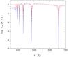 |
Fig. 2 Value of the Rosseland optical depth at which the plasma becomes optically thin (τλ = 1) at a particular wavelength for 1D model atmospheres at 6000 (red, solid), 10 000 (black, dotted) and 12 000 K (blue, dashed). |
2.2. Treatment of convection
One aspect that could explain differences between the LHD and standard structures is a difference in the physical parameters that are allowed to vary. Unfortunately, we discovered such incompatibility which is related to the MLT convection input parameters used to compute LHD structures. The LHD code setup in this study relies on the ML2/α = 0.8 parameterisation of the MLT that is used in the most recent white dwarf models (Tremblay et al. 2010), where the calibration of the mixing-length parameter α results from a comparison of near-UV and optically determined Teff. For completeness, we summarise in Table 1 the a,b and c parameters that are used to define the ML2 treatment of the MLT equations (see, e.g., Mihalas 1978; Tassoul et al. 1990; Bergeron et al. 1992b; Koester et al. 1994; Ludwig et al. 1999). There is a fourth parameter that was introduced early in the usage of the MLT theory (Vitense 1953) to allow for optically thin convective cells (see Eq. (7.72) of Mihalas 1978). This parameter is defined as d in the white dwarf field (see Eq. (4) of Bergeron et al. 1992b), and a f4 parameter, specified in a different way but recovering the Mihalas (1978) relation if f4 = 2, is defined in Table A1 of Ludwig et al. (1999). By changing the value of f4, the convective efficiency is modified in the transition between the optically thin and thick regions, which is the region of line formation. Therefore, this extra parameter can have a major effect on the predicted structures and spectra.
Adopted parameterisation of MLT.
In Paper I, the LHD models were computed with optically thick convective cells (f4 = 0) while in the present work, LHD models are allowed to have optically thin cells (f4 = 2). As a result the LHD code is now based on an implementation of the MLT theory that is exactly the same as in commonly used white dwarf models. The effect on the 3D log g corrections is discussed in Sect. 4. We point out that 3D simulations are completely unaffected by the MLT parameterisation.
3D model atmospheres.
2.3. Numerical precision
Finally, we had to increase the numerical precision in order to provide the best match between the LHD and standard structures. We found that at least 200 depth points must be used with the LHD code in order to recover the Tremblay et al. (2011a) structures. Furthermore, we find with both codes that the equation of radiative transfer must be solved for at least five angles. We stress that our results in terms of the numerical precision of the LHD code can not easily be transferred to the CO5BOLD code, because of the completely different treatment of convection. Instead, we show in Sect. 4.3 that the sensitivities of the 3D structures to different numerical parameters is very small and we conclude that our CO5BOLD code setup provides the required high precision.
3. 3D model atmospheres
We have computed a set of twelve 3D DA model atmospheres with the CO5BOLD code1 covering the range 13 000 > Teff (K) > 6000 at log g = 8.0. Table 2 gives a summary of the properties of these simulations. We have used the new EOS and opacity tables that were discussed in Sect. 2. We relied upon four different opacity tables, with the opacity bins sorted based on a 6000, 8000, 10 000 and 12 000 K 1D reference model atmosphere, respectively. The implementation of the boundary conditions is described in detail in Freytag et al. (2012, see Sect. 3.2) and CO5BOLD solar models rely on the same conditions. In brief, the lateral boundaries are periodic, and the top boundary is open to material flows and radiation. The bottom layer is open to convective flows (and radiation) in all but the three hottest simulations, and a zero total mass flux is enforced. We specify the entropy of the ascending material to obtain approximately the desired Teff value (derived from the emergent stellar flux). The entropy of the deep layers is increasing monotonically with Teff, hence there is a unique relation between the entropy at the bottom boundary and the effective temperature of a simulation. This control of the Teff of a model (i.e. the temporal and spatial average of the emergent radiative flux) is indirect and Teff is not an input parameter2. In contrast, the bottom layer is closed with imposed zero vertical velocities (but open to radiation) for the three hottest simulations, in which case we impose the radiative flux according to the diffusion approximation.
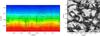 |
Fig. 3 Snapshot of the 3D white dwarf simulation at Teff ~ 8000 K and log g = 8. Left: temperature structure for a slice in the horizontal-vertical xz plane through a box with coordinates x,y,z (in km). The temperature is colour coded from 14 000 (red) to 3000 K (blue). The arrows represent relative convective velocities, while thick lines correspond to contours of constant Rosseland optical depth, with values given in the figure. Right: emergent bolometric intensity at the top of the horizontal xy plane. The rms intensity contrast with respect to the mean intensity is 7.6%. The length of the bar in the top right is 10 times the pressure scale height at τR = 2/3. |
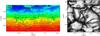 |
Fig. 4 Similar to Fig. 3 but for the simulation at Teff ~ 10 000 K. Left: the temperature is colour coded from 17 000 (red) to 5000 K (blue). Right: the rms intensity contrast is 14.4%. |
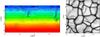 |
Fig. 5 Similar to Fig. 3 but for the simulation at Teff ~ 12 000 K. Left: the temperature is colour coded from 60 000 (red) to 7000 K (blue). Right: the rms intensity contrast is 18.8%. |
We typically started our simulations by scaling approximately another model from the grid. As long as the programme runs smoothly, the initial structure does not matter much (Freytag et al. 2012) for space- and time-averaged quantities. We first computed grey models for 10 s, and then switched on the non-grey radiative transfer for 10 s or more. More details about the time evolution of our simulations is given is Sect. 3.3.
We adopt a grid of 150 × 150 × 150 points in the x,y and z directions, where z is used for the vertical direction and points towards the exterior of the star. Compared to the simulations computed in Paper I, the vertical number of points was increased from 100 to 150. The geometrical dimensions are given in Table 2. We fixed the bottom layer at log τR = 3 for all simulations, well below the photosphere3. One exception is the third hottest model (Teff ~ 12 000 K) for which we recomputed a more extended simulation with a bottom boundary at log τR = 3.1. The bottom of the convective zone was too close to the simulation boundary at log τR = 3.0, which was artificially damping the convective velocities by a small amount. Nevertheless, we find that our two simulations with an unequal vertical extent show very little differences except for the sub-photospheric convective velocities. In all models, the top boundary reaches a space- and time-averaged value of no more than log τR ~ − 5. In Table 2 we also show the number of pressure scale heights between the photosphere and the bottom boundary that are covered by the simulations. It demonstrates that convective eddies reaching the photosphere are unlikely to be impacted by boundary conditions. The grid spacing in the z direction is non-equidistant. The horizontal geometrical dimensions are further in discussed in Sect. 3.4.
In terms of solving the hydrodynamical equations, the van Leer slope limiter was used in Paper I, but we have now switched to a less dissipative 2nd-order reconstruction method. Furthermore, regarding the time integration scheme, we now adopt the corner-transport upwind (CTU) method (Colella 1990).
It is well known that the flows in stellar atmospheres are characterized by very large Reynolds numbers (Re > 1010), and white dwarfs are not an exception. This implies that the flows are highly turbulent, and that the turbulent kinetic energy is then dissipated into heat at the Komolgorov microscale (d ~ HpRe− 3/4), i.e. on scales much smaller than the resolution of our grid. As a consequence, only the largest flow structures are resolved, and the small-scale kinetic energy is dissipated at the grid scale, either by the Roe solver itself or by an additional artificial tensor viscosity. The granules are the large flow structures that contribute to the global convective energy exchanges in the atmospheres, and as long as they are well resolved, the numerical treatment of the energy dissipation at smaller scales has very little effect on the predicted structures. Hence, viscosity is not a free parameter like, for instance, the mixing-length parameters. In Paper I, artificial viscosity was added, but with our new setup of the numerical schemes, we could compute all simulations without this explicit viscosity. This allows resolving a bit further the flows for which the spatial scale is close to the resolution of the box. Finally, we note that the radiation pressure is negligible for these models.
Figures 3 to 5 present the final snapshots for three of our simulations at Teff ~ 8000, 10 000 and 12 000 K. The first series of plots (left panels) presents the atmospheric structures in terms of temperature contours and velocity fields as a function of the geometrical depth (z) and one of the horizontal direction (x). We also show surfaces of constant Rosseland optical depth over which the mean structures are computed throughout this study.
In all snapshots, significant velocities are observed in the upper layers (τR ≲ 10-3) even though these regions are stable to convection. The presence of oscillating waves is the main explanation for this behaviour, and it is difficult to differentiate these waves from the exponentially decaying convective flows (overshoot layer), which transport energy outside of the convective zone (see Sect. 3.2). Another obvious observation is that the velocity field is significantly different for the hotter 12 000 K simulation. It is seen that the downdrafts are concentrated in narrow lanes in comparison to the cooler models. Furthermore, roughly the lower third of the 12 000 K simulation, in terms of geometrical depth, is stable to convection. However, large downdrafts, such as the one on the far right of Fig. 5, reach high τR values. The root-mean-square (rms) vertical velocities actually remain well above zero up to τR ~ 103 because of these downdrafts.
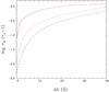 |
Fig. 6 Similar to Fig. 2 but in the wavelength range, with respect to the line centre, of the red wing of Hδ. |
The second series of plots (right panels) presents the emergent frequency integrated (bolometric) intensity. It is shown that the granulation size is changing significantly over the range of Teff. Once again, the 12 000 K simulation stands out with narrower cool downdrafts and smoother hot cells. The size, shape and contrast of the granulation patterns will be discussed in more detail in Sect. 3.4.
3.1. Mean structures
We have shown in Sect. 2 that by using the proper EOS and opacity tables, it is possible to reproduce standard white dwarf model atmospheres with the LHD code. Given that CO5BOLD employs the same microphysics and radiative transfer schemes as LHD, we can conclude that CO5BOLD reaches a similar precision, and possibly a better accuracy due to the improved convection treatment, in comparison to the current 1D models. We now compare directly the results from the 3D simulations with the 1D models of Tremblay et al. (2011a).
It was demonstrated in Paper I (Fig. 4) that in the case of DA white dwarfs, 3D spectral synthesis produces the same result as computing one ⟨ 3D ⟩ spectrum from a single ⟨ 3D ⟩ structure, which is the temporal and spatial average of a 3D simulation over surfaces of constant Rosseland optical depth. The mean temperature and pressure structures, and the atmospheric parameters (Teff and log g), are the quantities necessary to produce model spectra from the 3D simulations, which is the objective of Sect. 4. We derived mean T and P values from the average of T4 and P over surfaces of constant τR. We selected 12 random snapshots in the last 2.5 s of the simulations to make the temporal average. We determined the Teff values identified in Table 2 from the mean emergent flux of the 12 snapshots selected for the τR average. The rms variation of Teff with time is always much less than 1%. In contrast, log g is a fixed quantity in the hydrodynamical equations.
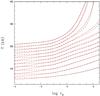 |
Fig. 7 Temperature structures versus log τR for ⟨ 3D ⟩ (red, solid) and 1D (black, dashed) model atmospheres. The temperature scale is correct for the 6000 K model (bottom curve), but other structures are shifted by 1 kK relative to each others for clarity. |
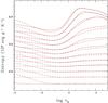 |
Fig. 8 Entropy as a function of log τR for our sequence of ⟨ 3D ⟩ (red, solid) and 1D models (black, dashed), with the coolest model at the bottom, and the hottest model at the top. The entropy scale is correct for the 6000 K model, but other structures were shifted by 0.1 unit for clarity. |
To understand the differences between ⟨ 3D ⟩ and 1D models, it is useful to look at other mean quantities. Therefore, we computed the mean entropy and rms velocities at constant optical depth, and different energy fluxes described below at constant geometrical depth. Figure 6 illustrates that the characteristic depth of the formation of Hδ, taken as a typical line, is within the range − 2 < log τR < 0. Hence this region of the photosphere is the most critical for the predicted spectra.
In Figs. 7 and 8, we compare the ⟨ 3D ⟩ and 1D structures in terms of the temperature and entropy, respectively. The 1D models are drawn from the grid of Tremblay et al. (2011a) with the ML2/α = 0.8 parameterisation of the MLT. Compared to the temperature, the entropy values are more sensitive to differences between ⟨ 3D ⟩ and 1D structures. Furthermore, the presence of a negative or positive entropy gradient (as a function of τR) shows whether a layer is stable or unstable to convection, respectively. It is observed that in stability terms, the top of the convective zone, and even the bottom of the zone for the three hottest structures, are at similar optical depths in ⟨ 3D ⟩ and 1D models. In the upper part of the atmospheres, the entropy gradient (in absolute value) and the temperatures are always much smaller in ⟨ 3D ⟩ structures, which is the result of convective overshoot. This overshoot layer is able to cool the upper layers because of a weak radiative coupling (see Sect. 3.3). In comparison, the 1D models are stable to convection and in radiative equilibrium.
In Fig. 9, we present the ratio of the convective flux to the total energy flux as a function of optical depth. The convective flux is the sum of the enthalpy, gravitational energy and kinetic energy fluxes. The shape of the convective zones as described by the convective flux is also similar between ⟨ 3D ⟩ and 1D models. One reason is that the overshoot in the upper layers acts in optically thin regions, and transports very little flux. For the three hottest models, however, the convective zone is systematically deeper for the ⟨ 3D ⟩ models in part because an overshoot layer is present at the bottom of the convection zone where it is able to transport energy. This is in qualitative agreement with the results from pulsation studies in which a slightly more efficient MLT parameterisation (ML2/α = 1.0) is used to describe the bottom of the convective zones (Fontaine & Brassard 2008). We note that larger than average differences in the ⟨ 3D ⟩ and 1D temperature structures at log τR > 1 for the hot models are due to the transition from convective to radiative layers. In general, the transition region from convective to radiative flux transport is smoother in ⟨ 3D ⟩ structures according to Fig. 9, which explains why ⟨ 3D ⟩ structures have smoother temperature gradients in the photosphere as reported by Fig. 7.
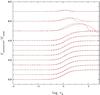 |
Fig. 9 Ratio of the convective to the total energy flux as a function of log τR for our sequence of ⟨ 3D ⟩ (red, solid) and 1D models (black, dashed), with the coolest model at the bottom, and the hottest model at the top. The ratio is exact for the 6000 K model, but other structures were shifted by 0.5 up to 11 500 K, and by 1.0 above that temperature, for clarity. |
Interestingly, the ⟨ 3D ⟩ and 1D models are the most similar at the boundaries of our computed sequence and the maximum differences between 1D and ⟨ 3D ⟩ models in the photosphere are detected in the middle of our sequence at Teff ~ 9000 − 10 000 K. At Teff ~ 6000 K, convection is almost fully adiabatic everywhere in the atmosphere, and since 1D and 3D models are based on the same input microphysics, it is expected that the adiabatic gradient, hence the structures, will be the same. For the hottest model (Teff ~ 13 000 K), the maximum convective flux becomes small, and the atmosphere is leading towards the fully radiative regime. Nevertheless, it is remarkable that the entropy gradients are still substantially different in the upper layers, which suggests that the convective overshoot is still significant at this temperature. However, part of the differences between the 1D and 3D Teff structures may also be caused by the distinct treatment of the radiative transfer.
3.2. Convective velocities
Another relevant aspect of the 3D simulations are the convective velocities. We present the rms vertical and horizontal velocities in Figs. 10 and 11. Due to the symmetry of the simulations, x and y velocities are nearly identical and we only show the former component. Our sequence of models exhibits smooth changes of the velocities between adjacent Teff values, which further confirms that our structures are well converged. The vertical velocities in Fig. 10 are the most interesting since we can relate them to the convective energy flux. The maximum vertical velocities are observed in the 11 500 and 12 000 K simulations and the values decrease in a regular way in cooler and hotter models. The velocities in the coolest computation at 6000 K are only a small fraction of the maximum velocities observed in our sequence, which illustrates the fact that only mild convection is needed to transport the small total energy flux at 6000 K.
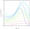 |
Fig. 10 Vertical rms velocity vz as a function of log τR for our sequence of ⟨ 3D ⟩ models from 6000 (lowest, red curve) over 10 000 (top, light blue curve) to 13 000 K (dark blue curve). |
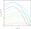 |
Fig. 11 Horizontal rms velocity vx as a function of log τR for our sequence of ⟨ 3D ⟩ models from 6000 (lowest, red curve) to 13 000 K (dark blue). |
The overshoot layer at the bottom of the convective zones is clearly seen in terms of the convective velocities. For the three hottest simulations, the velocities remain clearly above zero even at the bottom of the simulations (log τR ~ 3) while Fig. 8 shows, from the change of sign in the entropy gradient, that the layers become stable to convection at log τR ~ 1.1, 1.5 and 2.2 for the 13 000, 12 500 and 12 000 K simulations, respectively. Clearly, the overshoot layers extend, in log τR, at least 1 dex and up to 2 dex below the region unstable to convection. However, Fig. 9 illustrates that the overshoot layers transport very little convective energy flux except in the vicinity of the convective zone. Clearly, the relevance of the overshooting depends on the physical processes that are studied. For instance, we believe that in diffusion or convective mixing studies, a proper account of the overshoot layer is essential, as also concluded by Freytag et al. (1996) from 2D simulations.
Figures 10 and 11 would also suggest large overshoot layers above the convective zone, but we must be very cautious about this interpretation. Indeed, p-mode oscillations, with periods that are related to the geometry of the computational box (and boundary conditions), occur in all of our calculations. The effect of these oscillations is largely removed from all the mean quantities by the temporal average, except in the case of rms velocities. The amplitude of the p-mode oscillations is larger in the upper layers, where the pressure restoring force is lower (v ∝ P− 1/2 for undamped oscillations). In Fig. 10, the increase of the vertical velocities at log τR < − 2 is caused by these oscillations. Methods have been proposed to filter these oscillations (Ludwig et al. 2002) in order to look at the exponential overshoot more clearly. However, for the purpose of this work, the effect of overshooting into the upper layers can be more easily seen from the temperature and entropy structures.
The turbulent pressure  is a significant fraction of the local gas pressure in convective white dwarfs. This fraction reaches values of ~10% for the hottest simulations of our grid. The turbulent pressure derived from the RHD simulations illustrates the deviation from hydrostatic equilibrium. A proper account of the turbulent pressure in hydrostatic 1D models might help to improve the agreement between 1D and ⟨ 3D ⟩ structures.
3.3. Characteristic timescales
We note that three of our simulations (12 500 > Teff (K) > 11 500) are within the ZZ Ceti instability strip (Gianninas et al. 2011). It would be adequate to rely on our 3D structures as input for asteroseismic studies although the coolest ZZ Ceti star in our grid (11 500 K) is still convective at the bottom of the simulation. One option would be to compute RHD simulations that reach the bottom of the convective zone for all pulsating white dwarfs and then combine the RHD results with 1D interior structures. Such an application has been performed once by Gautschy et al. (1996) and it would be appropriate to update this analysis with our improved and less dissipative 3D calculations. Alternatively, Ludwig et al. (1999) have shown that it is generally possible to match a 3D structure including a convective bottom layer with an unique 1D structure model by relying on the asymptotic value of the spatially resolved entropy.
The study of time-resolved white dwarf model atmospheres with hydrodynamical simulations is unparalleled by 1D models. We note that this time resolution is of interest for asteroseismic studies. It has been understood long ago that convective processes were fairly rapid in ZZ Ceti white dwarfs compared to the typically observed pulsation periods in the range of 100−1000 s (Fontaine & Brassard 2008). As a consequence, non-adiabatic pulsation codes have adopted the concept of instantaneous reaction of the convection to the pulsations (Brassard & Fontaine 1997). The impact of time-resolved convection on asteroseismology of ZZ Ceti stars has recently been studied by van Grootel et al. (2012) using perturbations in the mixing-length equations. However, they show that the differences are small compared to the instantaneous reaction approximation.
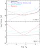 |
Fig. 12 Timescales for the ⟨ 3D ⟩ structure of a 12 000 (top panel) and 8000 K (bottom panel) DA white dwarf as a function of log τR. The different timescales are identified in the legend, and correspond to the advective timescale (black, solid), the Kevin-Helmholtz timescale (blue, dotted), the Brunt-Väisälä timescale (cyan, short dashed) and the radiative timescale (red, long dashed). |
In Fig. 12, we present four characteristic timescales as a function of the optical depth in the atmosphere of a 12 000 and 8000 K white dwarf. The timescales have been evaluated under simplifying assumptions, and should therefore be taken as order-of-magnitude estimates only. The timescales are defined as follow (see also Ludwig et al. 2002; Freytag et al. 2012): 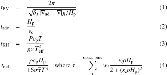 where
where  denotes the thermal expansion coefficient at constant pressure, ∇ad the adiabatic gradient, ∇ the actual temperature gradient, vc the rms convective velocity, cp the specific heat per gram, σ the Stefan-Boltzmann constant.
  is the characteristic optical depth of a disturbance of a size Hp, with κi the mean bin opacity per gram, and wi the weight of the opacity bin (see Eq. (A.4) of Ludwig & Kučinskas 2012).
First of all, the Brunt-Väisälä timescale (tBV) is related to the period of the oscillations due to the buoyancy force in regions stable to convection and the convective growth time for convectively unstable regions. The spikes observed for this quantity are related to the boundaries of the convective layers. The advective timescale (tadv), or the turnover timescale inside the convection zone, is related to the characteristic time for a convective mass element to move a distance of one pressure scale height. This timescale varies with depth from 10-2 to 1 s and it does not change significantly between the 8000 and 12 000 K simulations.
The Kelvin-Helmholtz timescale (tKH) is the thermal energy content (per unit area) divided by the total energy flux and describes the thermal relaxation (trough radiative diffusion). This timescale reaches values of the order of 15 s for the deeper layers of both the 8000 and 12 000 K models. However, in simulations below 12 000 K, the bottom layer is convective, and close to 100% of the flux is transported by convection. When the convective flux is much larger than the radiative flux at the bottom layer, the structure of the atmosphere is expected to adjust on the advective timescale. For the three hottest simulations with a radiative bottom layer, we have verified that in practice, the total flux is stable after a few seconds of computation in all layers, perhaps due to the presence of convective overshoot and a correct initial guess of the structure of the deepest layers.
The radiative timescale (trad) refers to the characteristic time for the decay of local temperature perturbations through radiative transfer. The radiative timescale is of the order of the advective timescale at 12 000 K, which is also the case for the 8000 K model, but only in the photosphere. The Péclet number in the photosphere, which is the ratio of the radiative timescale to the advective timescale, is changing from a value above to below unity between the cooler and hotter simulations, respectively. This implies that the evolution of convective cells in the photosphere will be largely influenced by radiation in the hot models in our grid, whereas for the cool models, convective cells are more directly governed by quasi-adiabatic expansion and compression. In the convective zone of the 12 000 K simulation, characteristic of a ZZ Ceti star, all timescales are lower than one second, which confirms that the reaction of the convective zone to changing conditions in the radiative layer just below will be rather instantaneous on the timescales of the pulsations.
In the 8000 K model, the radiative timescale is rather large at the top and bottom layers. At the bottom layer, energy is transported by convection and the large radiative timescale simply implies that the energy in the convective cells will hardly be lost by radiation. The upper layers above log τR ~ − 0.5 are, however, stable to convection. Hence Fig. 12 suggests that these layers may take up to 100 s to reach radiative equilibrium. The radiation field becomes weaker in cooler white dwarfs, and the decreasing line opacity creates upper layers that do not interact much with radiation. This contributes in creating the long observed radiative timescales. A similar phenomenon was observed for metal-poor dwarfs (Asplund & Garcia Perez 2001).
To make sure that our simulations have relaxed in the upper layers, we performed non-grey 2D simulations for 50 s for the three models between 7000 and 9000 K, and for 90 s for the model at 6000 K. The upper layers never actually reach a radiative equilibrium like in the 1D models. Instead the convective overshoot causes the entropy gradient in the upper layers to relax to a near-adiabatic structure, as seen in Fig. 8. We used the final 2D structures as initial conditions4 for the much more time consuming non-grey 3D simulations.
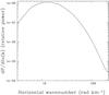 |
Fig. 13 Mean power spectrum as a function of the horizontal wavenumber (2π/λ) averaged over 250 snapshots of the (bolometric) intensity map of the 10 000 K 3D simulation. |
All non-grey 3D simulations were run for 10 s, which ensures that we typically cover about 100 advective timescales in the photosphere. We have verified that all simulations are relaxed in the last five seconds of computation and that they show no systematic and non-oscillatory change of their properties in all layers. We note that the four cooler simulations might still have an imprint of the 2D initial conditions in the upper layers because of the large radiative timescales.
The numerical time step is limited by the global minimum of the radiative and Courant-Friedrichs-Lewy timescales (tCFL = Δx/ [cs + vc], where cs the adiabatic sound speed). The latter corresponds the travel time of the shortest wave across a grid cell of dimension Δx. Typically, our time steps are of the order 10-4 − 10-5 s, and therefore the total number of steps is tsim/Δt ~ 105 − 106.
3.4. Characteristic length scales
We have previously discussed the vertical extent of our simulations which is naturally derived from our requirement to have the full atmospheres. However, the horizontal dimensions of the simulations are not well defined a priori. The 3D simulations have horizontal sizes, while such thing does not exist in 1D plane-parallel models. From physical considerations in the formation, transport and dissipation of convective cells, one can assume that the vertical size of the cells will be of the order of the local pressure scale height. However, calculations of stellar RHD models have shown that granular patterns have larger horizontal dimensions of the order of 10 times the local value of Hp (Freytag et al. 1997).
In Fig. 13, we present the power spectrum as a function of the horizontal wavenumber, for the emergent intensity in 250 different snapshots of the 10 000 K simulation (Fig. 4 gives one example of a snapshot). We display power per logarithmic wavenumber interval for a more direct identification of the power carrying scales (Ludwig et al. 2002). We remind the reader that the smallest wavenumber on the left in Fig. 13 represents a sinusoidal pattern with one hot crest and one cool crest (compared to the mean intensity). Ideally, our simulations should include at least of the order of 3 × 3 hot cells to have a good representation of the atmosphere, and have a sufficient resolution for each cell. We only qualitatively ensured that it was the case since we can derive the power spectra only after the simulations. The characteristic granulation is typically well resolved although because of the limitation of the Fourier analysis to identify granules and possible effects from the numerical parameters, the characteristic dimensions should be taken as estimates only. We note that we can not derive a single power law to describe the formation of smaller cells or sub-cells with a high wavenumber, much like in main-sequence simulations (Ludwig et al. 2002).
Figure 14 presents the characteristic size of the convective cells in our sequence of simulations, derived as the wavelength of the peak of the power spectra which we found were well fitted by a parabola. It is clearly seen that the cell dimensions are not well scaled by the pressure scale height in the photosphere, also shown in the figure. The characteristic size of the granulation patterns increases much more rapidly with Teff than what we would expect from simple thermodynamics considerations. The convective velocities and the associated Mach number are significantly increasing with Teff, and we suggest that it has an effect on the size of the convective cells by allowing for faster moving and thinner downdrafts. Furthermore, the timescales analysis of Sect. 3.3 suggests that the variation of the Péclet number is part of the explanation. The regime of regular bright and dark cells at cool temperatures (see, e.g., Fig. 3), where the advection dominates, change to the regime of large bright cells and narrow dark lanes at hotter temperatures (Fig. 5) when the radiation dominates.
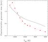 |
Fig. 14 Characteristic granular size (maximum of the mean power spectrum) as a function of Teff for our sequence of 3D simulations. The points are connected for clarity. The solid line is eight times the pressure scale height at τR = 2/3. |
Also of interest is the intensity contrast of the granulation patterns with respect to the mean intensity. This quantity can be derived from the intensity snapshots such as the ones shown in Figs. 3–5. The rms intensity contrast, a 3D effect that can not be easily predicted from existing 1D structures, is presented in Fig. 15. It is seen that the contrast varies from 1 to 20% in our sequence. In all but the three coolest models, the intensity contrast is in the 10–20% range. Very similar values of the intensity contrast are found for F, G and K dwarfs (see Fig. 15 of Freytag et al. 2012). We find that the granulation is visually similar in the Sun and a ~11 000 K white dwarf. In cooler white dwarfs, the granulation appears less structured in comparison to K main-sequence stars (see Fig. 3). We note that cool white dwarfs have a wide entropy minimum, which implies that the upper boundary of the convective zone is not well defined and that granulation patterns may form in a more extended optical depth range than dwarfs. This is a possible explanation for the fuzziness of granulation in cool white dwarfs. A careful study of the granulation patterns as a function of Teff, log g and metallicity for stars and white dwarfs would be useful to understand these structures.
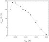 |
Fig. 15 rms intensity contrast divided by the mean intensity as a function of Teff for our sequence of 3D simulations. The points are connected for clarity. |
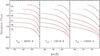 |
Fig. 16 Comparison of the blue wing of six Balmer line profiles (Hα to H8) calculated from ⟨ 3D ⟩ structures (red, solid) and standard 1D structures (black, dashed) for three models from our sequence identified in Table 2. Teff values are shown on the different panels. All line profiles were normalized to a unity continuum at a fixed distance from the line centre. All spectra were convolved with a Gaussian profile with a resolution of 6 Å to represent typical observations. |
We mention that at 13 000 K, the intensity contrast is still high, while the convective flux is fairly low according to Fig. 9. It appears that because the total energy flux is large in the atmosphere, large temperature differences are necessary to transport even a small amount of convective flux. However, the differences between 1D and ⟨ 3D ⟩ models are small according to Fig. 7. This may not be entirely surprising, since the weak convective flux is unlikely to have a global impact on the largely radiative structures. At the opposite cool end of our sequence, the 6000 K simulation features an intensity contrast of about 1%. It suggests again that convection is very efficient to transport the small total flux in this regime with only very small temperature variations. In between these two extremes, the increasing total flux contributes to enhance the contrast. Furthermore, as Teff is increasing, the Rosseland opacity is also increasing in the photospheres. This implies lower characteristic densities in the photospheres and higher convective velocities. This effect also contributes in enhancing the fluctuations.
Finally, we recall here that despite the significant variations in the spatially resolved intensity or flux, results of Paper I have shown that the mean wavelength-dependent flux is almost exactly equal to the same quantity computed from mean ⟨ 3D ⟩ structures. Hence the 3D fluctuations impact only indirectly the predicted spectra of white dwarfs through global modifications of the structures. In the following, the 3D simulations are therefore represented by their mean structures.
4. Astrophysical applications and discussion
4.1. Model spectra
Our sequence of 3D model atmospheres can be used as input for spectral synthesis as done in Paper I. We have shown in Sect. 2 that our 3D simulations are based on the same input microphysics as the standard 1D models, hence we can use the 1D model atmosphere code of Tremblay et al. (2011a) to compute ⟨ 3D ⟩ spectra, from ⟨ 3D ⟩ structures, that can be compared directly to observations. However, since our sequence of 3D calculations is limited to one log g value, we can not fit actual observations and we will still rely on a ⟨ 3D ⟩−1D differential approach to look at the 3D effects. We compare in Fig. 16 the ⟨ 3D ⟩ and 1D spectra for three characteristic simulations from our sequence of model atmospheres identified in Table 2. For clarity, only the blue wings of the lines are shown since the comparison is similar for the red wings. We must conclude, like in Paper I, that the differences are fairly subtle between the predicted ⟨ 3D ⟩ and 1D spectra, and that we must be careful about drawing conclusions about the atmospheric parameter corrections.
We find that the largest differences between ⟨ 3D ⟩ and 1D spectra are in the middle of our sequence, at Teff ~ 10 000 K, which is also the region where the structures are the most different (see Fig. 7) and where the high-log g problem is the most significant (see Fig. 1 of Paper I). One surprising result is that the higher lines of the series are significantly impacted by 3D effects. Since the higher series members are formed in a narrow region of the photosphere, one would expect that 3D effects decrease for these lines. The reason for this behaviour is that the strength of the higher lines is sensitive to the non-ideal effects (Hummer & Mihalas 1988; Tremblay & Bergeron 2009) in comparison to the lower lines. The non-ideal effects are in turn sensitive to the density in the atmospheres, and ⟨ 3D ⟩ structures have systematically cooler temperatures and higher densities in the upper layers due to the convective overshoot. These higher densities enhance the non-ideal effects and reduce the line strengths in comparison to the 1D predictions.
The cores of Hα and to a lesser degree Hβ are significantly deeper in ⟨ 3D ⟩ spectra. These cores are formed very high in the atmospheres, where the ⟨ 3D ⟩ structures deviate significantly from their 1D counterparts due to the overshoot cooling. Since spectroscopic analyses of white dwarfs with 1D models provide good fits to the line centres, the predictions from the ⟨ 3D ⟩ spectra should be regarded with caution. We believe that the lower temperatures predicted by our 3D simulations are real, although we can not rule out that shortcomings in radiative transfer or missing physics (e.g. magnetic fields or shock formation) might have an impact on this issue. We have verified with the TLUSTY code (Hubeny & Lanz 1995) that the 1D NLTE effects are restricted to the very centre of the lower lines (Δλ < 1 Å) in this regime of Teff and that they contribute to further enhance the absorption. Therefore, it seems unlikely that NLTE effects can help in explaining the differences between ⟨ 3D ⟩ and 1D line cores. As a conservative measure, we remove the line centres (| Δλ | < 1.5 Å) in our derivation of the 3D atmospheric parameter corrections.
4.2. Application to the high-log g problem
We derive here 3D atmospheric parameter corrections that are defined as the differences in Teff and log g when we fit the normalized line profiles of the ⟨ 3D ⟩ spectra with our grid of standard 1D models. More specifically, the corrections are defined as 1D−⟨ 3D ⟩, since we are interested in how much the atmospheric parameters of real stars would change when using ⟨ 3D ⟩ model spectra. In Fig. 17 and in Table 2, we present the 3D log g corrections. As in Paper I, we find that the corrections are negative for all spectra (i.e., the 3D simulations predict lower surface gravities), which is in the appropriate direction to correct the high-log g problem. We note that the 3D log g corrections are smaller in absolute value than those found in Paper I in the range of Teff in common between both studies, i.e. the four hottest simulations. This is a direct consequence of the fact that the 1D LHD models used in Paper I had optically thick convective cells everywhere in the atmosphere and were inconsistent with standard 1D models (see Sect. 2.2).
Also given in Fig. 17 are the observed shifts in log g derived from the spectroscopic analyses of the DA white dwarfs in the Sloan Digital Sky Survey (Tremblay et al. 2011a) and White Dwarf Catalog (Gianninas et al. 2011). These shifts correspond to the corrections required, in a bin of 1000 K around the simulation temperature, to match the mean mass value obtained from hot DA stars. We can see that the 3D corrections describe well the shape of the high-log g problem, with maximum corrections at Teff ~ 10 000 K where the problem is the largest. Also, the 3D corrections have about the right amplitude everywhere to solve the high-log g problem. Knowledge of the 3D log g corrections at log g = 7.5 and 8.5, and ultimately the spectroscopic fit of observations will be necessary to further constrain the log g values predicted by the 3D simulations. However, our results confirm the conclusion of Paper I that 1D MLT convection is the main reason for the high-log g problem, and that 3D model atmospheres provide a more stable surface gravity distribution as a function of the effective temperature.
We find that the 3D Teff corrections are mild, with an average of −230 K for the simulations in our sequence, hence the 3D effects are mostly log g effects. We believe that an actual comparison with observations will be necessary to interpret further the Teff shifts.
4.3. Sensitivity to numerics
In order to understand the precision of our 3D simulations and the uncertainty of our log g corrections, we computed a series of 9 simulations with the same input parameters, except for one modification as given Table 3. All simulations were computed at Teff ~ 10 000 K and log g = 8 for 5 s (at least one order of magnitude larger than both trad and tadv in the photosphere), with the converged model from our regular sequence as the starting model. We derived the mean temperature and pressure structures from 6 snapshots, and computed spectra using the same approach as we did for our regular sequence. In Table 3, we present how the 3D log g corrections are changed by our modifications.
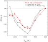 |
Fig. 17 3D log g corrections (red filled circles) as a function of Teff. In comparison, we show the shifts in surface gravity required to obtain a stable log g distribution as a function of Teff using the samples of the SDSS (open circles) and Gianninas et al. (2011; open squares). The points are connected for clarity. |
Sequence of 3D simulations with alternative parameters.
The first category of modifications (simulations A to G) can be classified as tolerable, i.e. from the physical constraints derived in this paper, these could be valid alternative input parameters for models in the regular sequence. We have A) increased the horizontal geometrical dimensions x and y by 25% (hence lowered the horizontal resolution); B) decreased the vertical resolution by using 100 grid points instead of 150; C) cut a section of atmosphere by changing the maximum value of log τR from 3.0 to 2.8; D) changed the top boundary condition by increasing by 10% the temperature of the incoming flow, E) used the Van Leer slope limiter, as in Paper I, instead of the less dissipative 2nd order method, F) used the more aggressive Piecewise Parabolic reconstruction (Colella 1984); and G) added artificial viscosity as in Paper I. According to Table 3, all of these modifications have no significant effect on the predicted gravities. This is a very important result, which confirms that the unresolved turbulent energy dissipation is not an issue for the predicted Balmer lines.
The simulations H and I include modifications that presumably result in a significantly less accurate account of the physical processes in comparison to the models in our regular sequence. We computed a 2D simulation by removing one of the horizontal direction. We find that the log g correction is changed by +0.06 dex, which is a moderate but significant effect. This result is meaningful since 2D models have been used in this work to provide relaxed upper layers for cool simulations (see Sect. 3.3). In fact, since 2D simulations are an order of magnitude faster to compute than 3D models, they are an interesting resource for applications where the geometrical dimensions or calculation times are larger than those in our sequence of 3D simulations. While these 2D calculations may not be as accurate as the 3D setup to predict the Balmer line spectra, they still appear to provide a very good physical description of the atmospheres. We note that early works on RHD models of white dwarfs were done with 2D simulations. Our result shows that their 2D approximation was adequate to derive white dwarf properties.
We close this section with the simulation I where we relied on the opacity table first computed by Ludwig et al. (1994) and also used in Paper I. We find that the log g correction is only changed by +0.03 dex. Therefore, we conclude that the opacity binning procedure was already very well tuned in previous works on RHD models of white dwarfs.
5. Conclusion
We computed a sequence of twelve 3D model atmospheres with the CO5BOLD radiation-hydrodynamics code. These simulations were made in the range 13 000 > Teff (K) > 6000 and at log g = 8 for pure-hydrogen atmospheres. We relied on EOS and opacity tables that have the same microphysics as in standard 1D models of white dwarfs, and we have verified that our models are expected to have the same precision as prevalent 1D structures. As a consequence, our sequence of 3D simulations is now expected to predict realistic absolute properties and can ultimately be compared with observations. We have demonstrated that the 3D simulations depend only weakly on numerical parameters by running a set of alternative simulations with modified parameters. This is unlike 1D models for which the free parameters in the mixing-length theory have a significant impact on the predicted structures.
We derived ⟨ 3D ⟩ spectra of the Balmer lines that we compared with those predicted from standard 1D white dwarf models. We found that the 3D log g corrections are the largest at around Teff ~ 10 000 K and that they have the right amplitude as a function of Teff to draw the conclusion that the source of the long-standing high-log g problem is the inability of the mixing-length theory to properly account for the convective energy transport. We will follow this study with the calculation of sequences of simulations at log g = 7.0, 7.5, 8.5 and 9.0. It will then be possible to apply the 3D model atmospheres in the spectroscopic analysis of DA white dwarf samples.
We rely on the January 2012 version of the code which is similar to the version described in Freytag et al. (2012). We utilise some new features that we describe in this section.
For clarity, we use round numbers in the discussion of the models in Table 2, but all calculations are done with the exact Teff values.
We define the photosphere as the line-forming regions as opposed to the atmosphere which is the full simulation.
We copied all quantities of the 2D snapshots in the third dimension, except for the velocities which were taken from a previously computed 3D snapshot.
Acknowledgments
P.-E.T. is supported by the Alexander von Humboldt Foundation. 3D model calculations have been performed on CALYS, a mini-cluster of 320 nodes built at Université de Montréal with the financial help of the Fondation Canadienne pour l’Innovation. We thank Prof. G. Fontaine for making CALYS available to us. We are also most grateful to Dr. P. Brassard for technical help. This work was supported by Sonderforschungsbereich SFB 881 “The Milky Way System” (Subproject A4) of the German Research Foundation (DFG). B.F. acknowledges financial support from the Agence Nationale de la Recherche (ANR), and the “Programme Nationale de Physique Stellaire” (PNPS) of CNRS/INSU, France.
References
- Allard, N. F., & Kielkopf, J. F. 1982, Rev. Mod. Phys., 54, 1103 [NASA ADS] [CrossRef] [Google Scholar]
- Allard, N. F., Kielkopf, J. F., & Loeillet, B. 2004, A&A, 424, 347 [NASA ADS] [CrossRef] [EDP Sciences] [Google Scholar]
- Asplund, M., & Garcia Perez, A. E. 2001, A&A, 372, 601 [NASA ADS] [CrossRef] [EDP Sciences] [Google Scholar]
- Asplund, M., Grevesse, N., Sauval, A. J., & Scott, P. 2009, ARA&A, 47, 481 [NASA ADS] [CrossRef] [Google Scholar]
- Bergeron, P., Wesemael, F., Fontaine, G., & Liebert, J. 1990, ApJ, 351, L21 [NASA ADS] [CrossRef] [Google Scholar]
- Bergeron, P., Saffer, R. A., & Liebert, J. 1992a, ApJ, 394, 228 [NASA ADS] [CrossRef] [Google Scholar]
- Bergeron, P., Wesemael, F., & Fontaine, G. 1992b, ApJ, 387, 288 [NASA ADS] [CrossRef] [Google Scholar]
- Bohlin, R. C. 2000, AJ, 120, 437 [NASA ADS] [CrossRef] [Google Scholar]
- Böhm-Vitense, E. 1958, ZAp, 46, 108 [NASA ADS] [Google Scholar]
- Brassard, P., & Fontaine, G. 1997, in Proc. 10th European Workshop on White Dwarfs, eds. J. Isern, M. Hernanz, & E. Gracia-Berro (Dordrecht: Kluwer), 214, 451 [Google Scholar]
- Caffau, E., & Ludwig, H.-G. 2007, A&A, 467, L11 [NASA ADS] [CrossRef] [EDP Sciences] [Google Scholar]
- Caffau, E., Ludwig, H.-G., Steffen, M., Freytag, B., & Bonifacio, P. 2011, Sol. Phys., 268, 255 [NASA ADS] [CrossRef] [Google Scholar]
- Colella, P. 1990, J. Comput. Phys., 87, 171 [NASA ADS] [CrossRef] [Google Scholar]
- Colella, P., & Woodward, P. R. 1984, J. Chem. Phys., 54, 174 [Google Scholar]
- Eisenstein, D. J., Liebert, J., Harris, H. C., et al. 2006, ApJS, 167, 40 [NASA ADS] [CrossRef] [Google Scholar]
- Finley, D. S., Koester, D., & Basri, G. 1997, ApJ, 488, 375 [NASA ADS] [CrossRef] [Google Scholar]
- Fontaine, G., & Brassard, P. 2008, PASP, 120, 1043 [NASA ADS] [CrossRef] [Google Scholar]
- Freytag, B., Ludwig, H.-G., & Steffen, M. 1996, A&A, 313, 497 [Google Scholar]
- Freytag, B., Holweger, H., Steffen, M., & Ludwig, H.-G. 1997, in Science with the VLT Interferometer, ed. F. Paresce (New York: Springer), 316 [Google Scholar]
- Freytag, B., Steffen, M., Ludwig, H.-G., et al. 2012, J. Comput. Phys., 231, 919 [Google Scholar]
- Gautschy, A., Ludwig, H.-G., & Freytag, B. 1996, A&A, 311, 493 [NASA ADS] [Google Scholar]
- Gianninas, A., Bergeron, P., & Ruiz, M. T. 2011, ApJ, 743, 138 [NASA ADS] [CrossRef] [Google Scholar]
- Girven, J., Gänsicke, B. T., Steeghs, D., & Koester, D. 2011, MNRAS, 417, 1210 [NASA ADS] [CrossRef] [Google Scholar]
- Hubeny, I., & Lanz, T. 1995, ApJ, 439, 875 [Google Scholar]
- Hummer, D. G., & Mihalas, D. 1988, ApJ, 331, 794 [NASA ADS] [CrossRef] [Google Scholar]
- Koester, D., Allard, N. F., & Vauclair, G. 1994, A&A, 291, L9 [NASA ADS] [Google Scholar]
- Koester, D., Kepler, S. O., Kleinman, S. J., & Nitta, A. 2009a, J. Phys.: Conf. Ser., 172, 012006 [Google Scholar]
- Koester, D., Voss, B., Napiwotzki, R., et al. 2009b, A&A, 505, 441 [NASA ADS] [CrossRef] [EDP Sciences] [Google Scholar]
- Kowalski, P. M., & Saumon, D. 2006, ApJ, 651, L137 [Google Scholar]
- Liebert, J., Bergeron, P., & Holberg, J. B. 2005, ApJS, 156, 47 [NASA ADS] [CrossRef] [Google Scholar]
- Ludwig, H.-G., & Kučinskas, A. 2012, A&A, 547, A118 [NASA ADS] [CrossRef] [EDP Sciences] [Google Scholar]
- Ludwig, H.-G., Jordan, S., & Steffen, M. 1994, A&A, 284, 105 [NASA ADS] [Google Scholar]
- Ludwig, H.-G., Freytag, B., & Steffen, M. 1999, A&A, 346, 111 [NASA ADS] [Google Scholar]
- Ludwig, H.-G., Allard, F., & Hauschildt, P. H. 2002, A&A, 395, 99 [NASA ADS] [CrossRef] [EDP Sciences] [Google Scholar]
- Mihalas, D. 1978, Stellar atmospheres, 2nd edn. (San Francisco: W. H. Freeman and Co.) [Google Scholar]
- Nordlund, Å. 1982, A&A, 107, 1 [NASA ADS] [Google Scholar]
- Steffen, M., Ludwig, H.-G., & Freytag, B. 1995, A&A, 300, 473 [Google Scholar]
- Tassoul, M., Fontaine, G., & Winget, D. E. 1990, ApJS, 72, 335 [Google Scholar]
- Tremblay, P.-E., & Bergeron, P. 2009, ApJ, 696, 1755 [NASA ADS] [CrossRef] [Google Scholar]
- Tremblay, P.-E., Bergeron, P., Kalirai, J. S., & Gianninas, A. 2010, ApJ, 712, 1345 [NASA ADS] [CrossRef] [Google Scholar]
- Tremblay, P.-E., Bergeron, P., & Gianninas, A. 2011a, ApJ, 730, 128 [NASA ADS] [CrossRef] [Google Scholar]
- Tremblay, P.-E., Ludwig, H.-G., Steffen, M., Bergeron, P., & Freytag, B. 2011b, A&A, 531, L19 (Paper I) [NASA ADS] [CrossRef] [EDP Sciences] [Google Scholar]
- Vitense, E. 1953, ZAp, 32, 135 [Google Scholar]
- Vögler, A., Bruls, J. H. M. J., & Schüssler, M. 2004, A&A, 421, 741 [NASA ADS] [CrossRef] [EDP Sciences] [Google Scholar]
- Weidemann, V., & Koester, D. 1980, A&A, 85, 208 [NASA ADS] [Google Scholar]
- van Grootel, V., Dupret, M.-A., Fontaine, G., et al. 2012, A&A, 539, A87 [NASA ADS] [CrossRef] [EDP Sciences] [Google Scholar]
All Tables
All Figures
|
Fig. 1 Atmospheric temperature as a function of the logarithm of the Rosseland optical depth for DA models with effective temperatures of 8000 (bottom) and 12 000 K (top). We show the standard 1D structures (solid black line) from Tremblay et al. (2011a), recomputed with a slightly higher numerical precision, and the improved 1D LHD structures (dashed blue line) described in the text. |
| In the text | |
|
Fig. 2 Value of the Rosseland optical depth at which the plasma becomes optically thin (τλ = 1) at a particular wavelength for 1D model atmospheres at 6000 (red, solid), 10 000 (black, dotted) and 12 000 K (blue, dashed). |
| In the text | |
|
Fig. 3 Snapshot of the 3D white dwarf simulation at Teff ~ 8000 K and log g = 8. Left: temperature structure for a slice in the horizontal-vertical xz plane through a box with coordinates x,y,z (in km). The temperature is colour coded from 14 000 (red) to 3000 K (blue). The arrows represent relative convective velocities, while thick lines correspond to contours of constant Rosseland optical depth, with values given in the figure. Right: emergent bolometric intensity at the top of the horizontal xy plane. The rms intensity contrast with respect to the mean intensity is 7.6%. The length of the bar in the top right is 10 times the pressure scale height at τR = 2/3. |
| In the text | |
|
Fig. 4 Similar to Fig. 3 but for the simulation at Teff ~ 10 000 K. Left: the temperature is colour coded from 17 000 (red) to 5000 K (blue). Right: the rms intensity contrast is 14.4%. |
| In the text | |
|
Fig. 5 Similar to Fig. 3 but for the simulation at Teff ~ 12 000 K. Left: the temperature is colour coded from 60 000 (red) to 7000 K (blue). Right: the rms intensity contrast is 18.8%. |
| In the text | |
|
Fig. 6 Similar to Fig. 2 but in the wavelength range, with respect to the line centre, of the red wing of Hδ. |
| In the text | |
|
Fig. 7 Temperature structures versus log τR for ⟨ 3D ⟩ (red, solid) and 1D (black, dashed) model atmospheres. The temperature scale is correct for the 6000 K model (bottom curve), but other structures are shifted by 1 kK relative to each others for clarity. |
| In the text | |
|
Fig. 8 Entropy as a function of log τR for our sequence of ⟨ 3D ⟩ (red, solid) and 1D models (black, dashed), with the coolest model at the bottom, and the hottest model at the top. The entropy scale is correct for the 6000 K model, but other structures were shifted by 0.1 unit for clarity. |
| In the text | |
|
Fig. 9 Ratio of the convective to the total energy flux as a function of log τR for our sequence of ⟨ 3D ⟩ (red, solid) and 1D models (black, dashed), with the coolest model at the bottom, and the hottest model at the top. The ratio is exact for the 6000 K model, but other structures were shifted by 0.5 up to 11 500 K, and by 1.0 above that temperature, for clarity. |
| In the text | |
|
Fig. 10 Vertical rms velocity vz as a function of log τR for our sequence of ⟨ 3D ⟩ models from 6000 (lowest, red curve) over 10 000 (top, light blue curve) to 13 000 K (dark blue curve). |
| In the text | |
|
Fig. 11 Horizontal rms velocity vx as a function of log τR for our sequence of ⟨ 3D ⟩ models from 6000 (lowest, red curve) to 13 000 K (dark blue). |
| In the text | |
|
Fig. 12 Timescales for the ⟨ 3D ⟩ structure of a 12 000 (top panel) and 8000 K (bottom panel) DA white dwarf as a function of log τR. The different timescales are identified in the legend, and correspond to the advective timescale (black, solid), the Kevin-Helmholtz timescale (blue, dotted), the Brunt-Väisälä timescale (cyan, short dashed) and the radiative timescale (red, long dashed). |
| In the text | |
|
Fig. 13 Mean power spectrum as a function of the horizontal wavenumber (2π/λ) averaged over 250 snapshots of the (bolometric) intensity map of the 10 000 K 3D simulation. |
| In the text | |
|
Fig. 14 Characteristic granular size (maximum of the mean power spectrum) as a function of Teff for our sequence of 3D simulations. The points are connected for clarity. The solid line is eight times the pressure scale height at τR = 2/3. |
| In the text | |
|
Fig. 15 rms intensity contrast divided by the mean intensity as a function of Teff for our sequence of 3D simulations. The points are connected for clarity. |
| In the text | |
|
Fig. 16 Comparison of the blue wing of six Balmer line profiles (Hα to H8) calculated from ⟨ 3D ⟩ structures (red, solid) and standard 1D structures (black, dashed) for three models from our sequence identified in Table 2. Teff values are shown on the different panels. All line profiles were normalized to a unity continuum at a fixed distance from the line centre. All spectra were convolved with a Gaussian profile with a resolution of 6 Å to represent typical observations. |
| In the text | |
|
Fig. 17 3D log g corrections (red filled circles) as a function of Teff. In comparison, we show the shifts in surface gravity required to obtain a stable log g distribution as a function of Teff using the samples of the SDSS (open circles) and Gianninas et al. (2011; open squares). The points are connected for clarity. |
| In the text | |
Current usage metrics show cumulative count of Article Views (full-text article views including HTML views, PDF and ePub downloads, according to the available data) and Abstracts Views on Vision4Press platform.
Data correspond to usage on the plateform after 2015. The current usage metrics is available 48-96 hours after online publication and is updated daily on week days.
Initial download of the metrics may take a while.