| Issue |
A&A
Volume 552, April 2013
|
|
|---|---|---|
| Article Number | A140 | |
| Number of page(s) | 25 | |
| Section | Extragalactic astronomy | |
| DOI | https://doi.org/10.1051/0004-6361/201220073 | |
| Published online | 17 April 2013 | |
Spectral energy distributions of H ii regions in M 33 (HerM33es) ⋆
1 Dept. Física Teórica y del Cosmos, Universidad de Granada, 18071 Granada, Spain
e-mail: This email address is being protected from spambots. You need JavaScript enabled to view it.
2 Instituto Radioastronomía Milimétrica (IRAM), Av. Divina Pastora 7, Núcleo Central, 18012 Granada, Spain
3 Department of Astronomy, University of Massachusetts, Amherst, MA 01003, USA
4 Institute for Astronomy, Astrophysics, Space Applications & Remote Sensing, National Observatory of Athens, P. Penteli, 15236 Athens, Greece
5 Aix Marseille Université, CNRS, LAM (Laboratoire d’Astrophysique de Marseille) UMR 7326, 13388 Marseille, France
6 Observatoire de Paris, LERMA, 61 Av. de l’Observatoire, 75014 Paris, France
7 Leiden Observatory, Leiden University, PO Box 9513, 2300 RA Leiden, The Netherlands
8 Max Planck Institut für Astronomie, Königstuhl 17, 69117 Heidelberg, Germany
9 Laboratoire d’Astrophysique de Bordeaux, Université Bordeaux 1, Observatoire de Bordeaux, OASU, UMR 5804, CNRS/INSU, BP 89, 33270 Floirac, France
10 IPAC, MS 100–22 California Institute of Technology, Pasadena, CA 91125, USA
11 Tata Institute of Fundamental Research, Homi Bhabha Road, 4000005 Mumbai, India
Received: 22 July 2012
Accepted: 23 January 2013
Abstract
Aims. Within the framework of the Herschel M 33 extended survey HerM33es and in combination with multi-wavelength data we study the spectral energy distribution (SED) of a set of H ii regions in the Local Group galaxy M 33 as a function of the morphology. We analyse the emission distribution in regions with different morphologies and present models to infer the Hα emission measure observed for H ii regions with well defined morphology.
Methods. We present a catalogue of 119 H ii regions morphologically classified: 9 filled, 47 mixed, 36 shell, and 27 clear shell H ii regions. For each object we extracted the photometry at twelve available wavelength bands, covering a wide wavelength range from FUV-1516 Å (GALEX) to IR-250 μm (Herschel), and we obtained the SED for each object. We also obtained emission line profiles in vertical and horizontal directions across the regions to study the location of the stellar, ionised gas, and dust components. We constructed a simple geometrical model for the clear shell regions, whose properties allowed us to infer the electron density of these regions.
Results. We find trends for the SEDs related to the morphology of the regions, showing that the star and gas-dust configuration affects the ratios of the emission in different bands. The mixed and filled regions show higher emission at 24 μm, corresponding to warm dust, than the shells and clear shells. This could be due to the proximity of the dust to the stellar clusters in the case of filled and mixed regions. The far-IR peak for shells and clear shells seems to be located towards longer wavelengths, indicating that the dust is colder for this type of object. The logarithmic 100 μm/70 μm ratio for filled and mixed regions remains constant over one order of magnitude in Hα and FUV surface brightness, while the shells and clear shells exhibit a wider range of values of almost two orders of magnitude. We derive dust masses and dust temperatures for each H ii region by fitting the individual SEDs with dust models proposed in the literature. The derived dust mass range is between 102−104 M⊙ and the cold dust temperature spans Tcold ~ 12−27 K. The spherical geometrical model proposed for the Hα clear shells is confirmed by the emission profile obtained from the observations and is used to infer the electron density within the envelope: the typical electron density is 0.7 ± 0.3 cm-3, while filled regions can reach values that are two to five times higher.
Key words: galaxies: individual: M 33 / galaxies: ISM / Local Group / dust, extinction / HII regions / ISM: bubbles
Appendices are available in electronic form at http://www.aanda.org
© ESO, 2013
1. Introduction
The interstellar regions of hydrogen ionised by massive stars are normally called H ii regions. The classical view of an H ii region is a sphere of ionised gas whose radius is obtained by the balance between the number of ionisation and recombination processes occurring in the gas. In a general picture the H ii region components are the central ionising stars, a bulk of ionised gas that can be mixed with interstellar dust, and a photodissociation region (PDR) surrounding the ionised gas cloud and tracing the boundaries between the H ii region and the molecular cloud (e.g. Osterbrock & Ferland 2006).
The properties of H ii regions can be described by the nature of the stellar population that ionises the gas and the physical conditions of the interstellar medium (ISM) where the stars are formed. Based on these two aspects, we find H ii regions with a broad range of luminosities, shapes, and sizes: from small single-ionised regions to large ensembles of knots of star formation intertwined with ionised gas filling the gaps between knots. The morphology of the regions, described by the appearance in Hα images, can therefore vary significantly from small concentrated Hα distributions to more diffuse shell-like structures.
The physical properties of H ii regions have been extensively studied observationally using Hα images, in order to obtain luminosity functions, mean electron density, and radii (e.g. Kennicutt 1984; Shields 1990); optical spectroscopy to obtain electron density and temperature, metallicity, and extinction (e.g. McCall et al. 1985; Vílchez et al. 1988; Oey et al. 2000; Oey & Shields 2000); or broad-band images that allow us to study the content of their stellar population (e.g. Grossi et al. 2010). All these different approaches can be combined to gain a better general picture of H ii regions.
Since the recent launch of the Spitzer telescope, a new wavelength window has been opened to analyse the physical properties of H ii regions. Numerous observational studies have been performed in nearby H ii regions where the spatial resolution of the Spitzer data allows us to differentiate between the emission distribution of the polycyclic aromatic hydrocarbon (PAH) features, described by the 8 μm Spitzer band and the emission of very small grains (VSG) given by the 24 μm Spitzer band (among others, for Galactic H ii regions, Watson et al. 2008; Paladini et al. 2012, for the Large Magellanic Cloud, Meixner et al. 2006; Churchwell et al. 2006, and for H ii regions in M 33, Relaño & Kennicutt 2009; Verley et al. 2009; Martínez-Galarza et al. 2012). Churchwell et al. (2006) reveal the existence of 322 partial and close ring bubbles in the Milky Way using infrared images from Spitzer, and they argue that the bubbles are formed in general by hot young stars in massive star-forming regions. In M 33, Boulesteix et al. (1974) presented a catalogue of 369 H ii regions over the whole disk of the galaxy and showed there are some ring-like H ii regions in the outer parts of the disk. These authors propose that these regions are late stages in the lives of the expanding ionised regions. HI observations of M 33 (Deul & den Hartog 1990) reveal HI holes over the disk of the galaxy: the small (diameters <500 pc) HI holes correlate well with OB associations and, to a lesser extent, with H ii regions; however, the large holes (diameters >500 pc) show an anti-correlation with H ii regions and OB associations. Expanding ionised Hα shells have been found in a significant fraction of the H ii region population in late-type galaxies (Relaño et al. 2005). This can be interpreted in terms of an evolutionary scenario where the precursors of the HI holes would be the expanding ionised Hα shells (Relaño et al. 2007, and see also Walch et al. 2012).
The high-resolution data from Herschel instrument (Pilbratt et al. 2010) cover a new IR-wavelength range that has not been available before. The combination of data from UV (GALEX) to IR (Herschel) offers us a unique opportunity to study the SEDs of H ii regions with the widest wavelength range currently available. Using new Herschel observations, recent studies of a set of Galactic H ii regions with shell morphology have already been performed (Anderson et al. 2012; Paladini et al. 2012). Within the Key Project HerM33es (Kramer et al. 2010), a set of H ii regions has been recently shown in the northern part of M 33 to have an IR emission distribution in the Herschel bands that clearly follows the shell structure described by the Hα emission (Verley et al. 2010). While there is no emission in the 24 μm band in these regions, cool dust emitting in the 250, 350, and 500 μm is observed around the Hα ring structure. The 24 μm emission distribution for these objects is very different from the distribution presented in large H ii complexes where a spatial correlation between the emission in the 24 μm band and Hα emission has been observed (e.g. Verley et al. 2007; Relaño & Kennicutt 2009).
Recently, a study of the star-forming regions in the Magellanic Clouds has analysed the relation of the amount of flux at the different wavelengths using SED analysis (Lawton et al. 2010). These authors find that the H ii region SEDs peak at 70 μm, and they have obtained a total-IR (TIR) luminosity from the SED analysis for each H ii region. Unfortunately, this study does not cover the optical and ultraviolet (UV) part of the spectrum, which is crucial for studying the amount of stellar radiation that can heat the dust.
We study here the dust emission distribution, as well as the dust physical properties, in a large sample of H ii regions in M 33, looking for trends with morphology. M 33, one of the disk galaxies in the Local Group with a significant amount of star formation, is the most suitable object to perform such as multi-wavelength study. The spatial resolution for the bands covering from UV (GALEX) to IR (Herschel, key project HerM33es, Kramer et al. 2010) allows us to study the interior of the H ii regions in this galaxy and to extract the SED of individual objects. The analysis will help us to better understand the interplay between star formation and dust in different H ii region types.
The paper is organised as follows. In Sect. 2 we present the data we use here, from UV (GALEX) to far-IR (FIR) (Herschel). Section 3 is devoted to explaining the methodology applied to select and classify the H ii region sample and to obtaining the photometry of the objects. In Sect. 4 we present the SEDs for each H ii region and draw conclusions on the SED trends related to the morphology of the objects, and in Sect. 5 we study the physical properties of the dust for H ii regions with different morphology. Section 6 is devoted to analysing the emission distribution of each band within the individual regions and to deriving the electron density for a set of the regions with different morphologies. In Sect. 7 we discuss the results, and in Sect. 8 we summarise the main conclusions of this paper.
2. The data
In this section we describe the multi-wavelength data set that has been compiled for this study. A summary of all the images used here, along with their angular resolutions is given in Table 1.
2.1. Far and near ultraviolet images
To investigate the continuum UV emission of M 33, we used the data from GALEX (Martin et al. 2005), in particular the data distributed by de Paz et al. (2007). A description of GALEX observations in far–UV (FUV, 1350–1750 Å) and near-UV (NUV, 1750–2750 Å) relative to M 33 and of the data reduction and calibration procedure can be found in Thilker et al. (2005). The angular resolution of these images is 4 4 for FUV and 54 for NUV.
Summary of the multi-wavelength set of data.
2.2. Hα images
To trace the ionised gas, we used the narrow-line Hα image of M 33 obtained by Greenawalt (1998). The reduction process, using standard IRAF1 procedures to subtract the continuum emission, is described in detail in Hoopes & Walterbos (2000). The total field of view of the image is 1.75 × 1.75 deg2 (2048 × 2048 pixels with a pixel scale of 203) with a 66 resolution.
The Hα image from the “Survey of Local Group Galaxies” (Massey et al. 2006) is used here to check for the existence of shells and to revise the morphological classification (see Sect. 3.1), because it has a much better angular resolution (08) and pixel scale (027). Unfortunately, this image is saturated in the central parts of the most luminous H ii regions, therefore the photometry has been extracted from the Hα image by Hoopes & Walterbos (2000).
2.3. Infrared images
Dust emission can be investigated through the mid-IR (MIR) and FIR data of M 33 obtained with the Spitzer Infrared Array Camera (IRAC) and Multiband Imaging Photometer (MIPS; Werner et al. 2004; Fazio et al. 2004; Rieke et al. 2004). The complete set of IRAC (3.6, 4.5, 5.8, and 8.0 μm) and MIPS (24, 70, and 160 μm) images of M 33 is described in Verley et al. (2007, 2009): the Mopex software (Makovoz & Khan 2005) was used to gather and reduce the basic calibrated data (BCD). We chose a common pixel size equal to 12 for all images. The images were background subtracted, as explained in Verley et al. (2007). The spatial resolutions measured on the images are 25, 29, 30, 30 for IRAC 3.6, 4.5, 5.8, 8.0 μm, respectively; and 63, 160, and 400 for MIPS 24, 70, and 160 μm, respectively. The complete field-of-view observed by Spitzer is very large and allows us to achieve high redundancy and a complete picture of the star-forming disk of M 33, despite its relatively large extension on the sky. The Herschel observations of M 33 were carried out in January 2010, covering a field of 1.36 square degrees. PACS (100 and 160 μm) and SPIRE (250, 350, and 500 μm) were obtained in parallel mode with a scanning speed of 20′′ s-1. The PACS reduction has been performed using the map-making software Scanamorphos (Roussel 2012) as described in Boquien et al. (2011). The SPIRE reduction has been done using the Herschel data processing system (HIPE, Ott 2010, 2011), and the maps were created using a “naive” mapping projection (Verley et al. 2010; Boquien et al. 2011; Xilouris et al. 2012). The spatial resolution of the Herschel data are 77 and 112 for PACS 100 μm and 160 μm and 212, 272, and 460 for 250 μm, 350 μm, and 500 μm, respectively. Due to the significant improvement in spatial resolution of the PACS images, we use here the PACS 100 μm and 160 μm images rather than the MIPS 70 μm and 160 μm.
3. Methodology
In this section we explain how the sample of H ii regions was selected and how we performed the photometry that allowed us to obtain the SED for each object.
3.1. Sample of H ii regions
We visually selected a sample of H ii regions and classified them to fulfil the following criteria: filled regions are objects showing a compact knot of emission, mixed regions are those presenting several compact knots and filamentary structures joining the different knots, and shells are regions showing arcs in the form of a shell. We added another classification for the special case where we saw complete and closed shells, these objects are called clear shells. We used the Hα image from Hoopes & Walterbos (2000) to select the regions and classify their morphology. In a further step, we checked for the classification with the high-resolution Hα image of Massey et al. (2006). From the 119 selected H ii regions, 9 are filled, 47 are mixed, 36 are shell, and 27 are clear shell H ii regions.
 |
Fig. 1 Location of the H ii region sample on the continuum-subtracted Hα image of M 33 from Hoopes & Walterbos (2000). The radii of the regions correspond to the aperture radii used to obtain the photometry. Colour code is as follows: filled (blue), mixed (green), shell (yellow) and clear shell (red) regions. |
In Fig. 1 we show the continuum-subtracted Hα image and the location of our H ii region sample. A colour code was used to show the different morphological classes: blue, green, yellow, and red stand for filled, mixed, shell, and clear shell H ii regions, respectively. An example of H ii regions for each morphology can be seen in Fig. 2, and the WCS coordinates, aperture size, and classification are presented in Table B.1.
 |
Fig. 2 Examples of H ii regions for each classification (see Sect. 3.1 for details on how the classification was performed). The circles correspond to the aperture used to obtain the photometry. The aperture radii are given in Col. 4 of Table B.1. |
The H ii region sample is by no means complete, since we chose a set of objects isolated enough to distinguish morphology. Therefore, we did not attempt to derive any results based on the completeness of the H ii region population of the galaxy, we instead inferred conclusions from the comparison of the SED behaviour of H ii regions with different Hα morphologies. Our sample of H ii regions presents common objects with previous M 33 source catalogues given in the literature. Using a tolerance of 120 pc, the 119 sources of the present study overlap with 45 H ii regions in Hodge et al. (1999), 7 star clusters in Chandar et al. (2001), 16 star clusters in Grossi et al. (2010), 67 sources selected at 24 μm Verley et al. (2007) and 38 Giant Molecular Clouds in Gratier et al. (2012). The main location difference with Hodge et al. (1999) and Verley et al. (2007) is that the present study have more objects towards the outskirts of the galaxy because we are selecting isolated H ii regions for which clear morphological classification can be carried out. The star clusters in common with Grossi et al. (2010) show ages between 1.5 and 15 Myr. In Fig. 3 we show the Hα (left) and 24 μm (right) luminosity distribution of our sample. The luminosities span a range of more than two orders of magnitude in Hα and 24 μm bands. The covered luminosity range of our sample is typical of the H ii regions of spiral galaxies (e.g. Rozas et al. 1996).
 |
Fig. 3 Histograms of the Hα (left) and 24 μm (right) luminosities of our H ii region sample and the aperture sizes used to perform the photometry. |
We defined the photometric apertures for each H ii region using the Hα image from Hoopes & Walterbos (2000) in order to include the total emission of the region. We also compared these apertures with the 24 μm image to ensure that the emission in this band was also included in the selected aperture. It is important to note that the H ii regions were selected in a visual way, choosing those that are isolated and have clear morphology. Therefore, the photometric aperture size is in some way arbitrary and defines what we think an H ii region is by showing one of the morphological types analysed in this study. The selected photometric apertures should not be confused with the actual sizes of the H ii regions. A histogram of the aperture radii of the classified H ii regions is shown in Fig. 4. There is a relation between the photometric aperture size and the morphology of the regions: while most filled regions have radii smaller than ~150 pc, the mixed ones are larger, followed by the shells with radii up to 250 pc. Clear shell regions have much larger radii, up to 270 pc. The large mixed H ii region with 280 pc radii is the largest star-forming region in M 33, NGC 604.
There is a relation between the location of the regions on the galaxy disk and the morphological classification. Most of the clear shells are seen in the outer parts of the galaxy (see e.g. the northern and western outer parts of Fig. 1). However, to check whether we are biased by the crowding effects near the centre of the galaxy while defining our sample, we created a set of ten fake shells with different radii and luminosities in our Hα image and redid the morphological classification. We were able to recover only one of the fake inserted shells. This simple exercise shows that our selection has been done to create a clear defined classification to study the trends of the SED with the morphology, rather than to attempt a study of the complete H ii region population of M 33.
3.2. Photometry
Owing to the spatial resolutions and pixel scales of the different images, we performed some technical steps before obtaining the photometry of the regions in each band. We first subtracted the sky level in each image when this task was not originally done by the instrument pipelines. Since the angular resolution of the SPIRE 350 and 500 μm maps are 272 and 460, respectively, we decided to discard them and used the SPIRE 250 μm as our reference map, degrading all the other maps of our set to a resolution of 212, the SPIRE 250 μm spatial resolution. Keeping a final resolution to better than 212 is important in this project since we want to be able to disentangle the structure of shells, which would disappear if we degrade our maps to a lower resolution. We also registered our set of images to the SPIRE 250 μm image, with a final pixel size of 6.0′′. Although we still could perform an analysis of the SEDs without the 250 μm data, the flux at this band is necessary in order to estimate the dust mass and dust temperature for the individual H ii regions (see Sect. 5).
The photometry was performed with the IRAF task phot. The total flux within the visually defined aperture of each source was measured in all the bands. To eliminate the contribution of the diffuse medium to the measured fluxes, we subtracted a local background value for each region. The local background is defined as the mode value of the pixels within a ring whose inner radii is located five pixels away from the circular aperture and with a five-pixel width. The mode was obtained after rejecting all the pixels with values higher than two times the standard deviation value within the sky ring. We chose different widths and inner radii to define the sky annulus and find differences in the sky values of ~5–20%. The regions with absolute fluxes lower than their errors were assigned an upper limit of three times the estimated uncertainty in the flux. Those regions with negative fluxes showing absolute values higher than the corresponding errors are discarded from the study. In Table B.2 we show the fluxes for each band, together with the corresponding errors.
 |
Fig. 4 Histogram of the H ii region photometric aperture radii of the classified object sample in M 33. The photometric aperture was defined using the Hα image from Hoopes & Walterbos (2000) (see Sect. 3.2 for more details). |
4. Spectral energy distributions
We obtained the SEDs for each H ii region in our sample. The result is shown in Fig. 5: in the left-hand panel we represent the total flux versus the wavelength, and in the right-hand panel we show the surface brightness (SB). The regions corresponding to each morphology are colour-coded: blue, green, yellow, and red correspond to filled, mixed, shell, and clear shell, respectively. The thicker lines correspond to the SEDs obtained using the median values at each band for all the H ii regions in each morphological sample. When calculating the median value at each band, the upper limit fluxes (see Sect. 3.2) were discarded.
 |
Fig. 5 SED for our set of H ii regions. Left panel: SEDs derived using the fluxes of the regions, a median value for the fluxes uncertainties is shown in the lower left corner. Right panel: surface brightness is used to obtain the SEDs. The thick lines correspond to the SEDs obtained using the median values at each band for all the H ii regions in each morphological sample. |
 |
Fig. 6 SED for our set of H ii regions normalised to the emission in the 24 μm band from Spitzer (left panel) and to the FUV emission from GALEX (right panel). The normalisation emphasises the IR part of the SED showing the different behaviours for filled and mixed regions and shell and clear shells objects. The thick lines correspond to the SEDs obtained using the median values at each band for all the H ii regions in each morphological sample. |
Several trends can be seen in these figures showing the difference in behaviour between the filled-mixed H ii regions and the shell-like objects. The H ii regions classified as mixed are the most luminous in all bands, which reflects that these H ii regions are formed by several knots of Hα emission and correspond to large H ii region complexes (see left panel of Fig. 5). However, in the right-hand panel of Fig. 5 we see that the filled and mixed regions are the ones with higher SB. Interestingly, the IR flux for filled, shells, and clear shells are very similar, but the SB of the shells and clear shells is lower than SB of filled and mixed regions. This could be interpreted by a pure geometrical argument because shells and clear shells cover a larger area than filled regions. Because the fluxes between the filled, shell, and clear shell regions is very similar (left panel of Fig. 5), but the SBs change (filled and mixed regions show similar SB, while the shells and clear shells show lower SB than the filled and mixed ones, see right panel of Fig. 5), we suggest that the filled regions could be the previous stages of the shell and clear shell objects. The explanation is that the total flux would be conserved in all the regions, but when the region ages and expands the SB lowers (as is happening for the shells and clear shells). Mixed regions would also fit in this picture as they are typically formed by several filled regions. Their total flux should be higher than the filled regions, but the SB should be the same as the filled regions.
Another interesting point that the SB SEDs show is the low SB at 24 μm for shells and clear shells (right panel of Fig. 5). The mixed and filled regions show higher emission of hot dust than the shells and clear shells, which may be due to the proximity of the dust to the power sources in the filled and mixed regions. Besides this, the slightly steeper slopes for the shells and clear shells between 24 μm and 70 μm imply that the relative fraction of cold and hot dust could be higher for shells and clear shells than for filled and mixed regions.
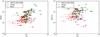 |
Fig. 7 Hα (left) and FUV (right) surface brightness as a function of P24. Colour code: red corresponds to shells and clear shells, blue to filled and green to mixed regions. |
The SED trends in the IR part of the spectrum are emphasised when we normalise the SEDs to the 24 μm fluxes (left panel of Fig. 6). Filled and mixed regions follow the same pattern and have the similar normalised fluxes in the MIPS, PACS, and SPIRE bands, while shells and clear shells have in general higher fluxes for these bands. In the right-hand panel of Fig. 6 we show the SED normalised to the FUV flux from GALEX. Filled regions show the highest FIR fluxes in this normalisation. This shows that in the filled regions the dust is so close to the central stars that it is very efficiently heated, while shells and clear shells present less fluxes in this normalisation because the dust is in general distributed farther away from the central stars. Also, in right-hand panel of Fig. 6 we see that the FIR peak for shells and clear shells seems to be located towards longer wavelengths, indicating that the dust is colder for this type of object. In a sample of 16 Galactic H ii regions Paladini et al. (2012) found that the SED peak of the H ii regions is located at ~70 μm, while the SEDs obtained with larger apertures including the PDR peak at ~160 μm. Indeed the SEDs of shells and clear shells might include a higher fraction of PDR, and thereby shifting the peak towards longer wavelengths. In a study of the SEDs for a set of H ii regions in the Magellanic Clouds, Lawton et al. (2010) also conclude that most of the SEDs peaks around 70 μm. Here we show that the peak of the IR SEDs is closer to the 100 μm band than to the 70 μm one. The behaviour of the SED in the IR part of the spectrum is studied in more detail in Sect. 5.2.
 |
Fig. 8 P24 (top) and P8 (bottom) versus R71 for DL07 dust models with qPAH = 0.47% (left column) and 4.6% (right column). A value of Umax = 106U has been considered for all models. Colour code: red corresponds to shells and clear shells, blue to filled, and green to mixed regions. |
5. Dust physical properties
In this section we apply models from (Draine & Li 2007, hereafter DL07) to study the contribution of the interstellar radiation field (ISRF) to the heating of dust for each H ii region type and to estimate the dust mass for each individual H ii region.
5.1. Analysis of the stellar radiation field
The ratio of the surface brightness in different IR bands may bring information about the dust properties. We devote this section to studying the properties of the dust for our objects and investigating possible relations between the dust properties and the region’s morphologies. To compare the emission of the dust in the IR bands, we subtracted the stellar emission in the 8 μm and 24 μm bands. We used the 3.6 μm image and the prescription given by Helou et al. (2004) to obtain a pure dust (non-stellar) emission at 8 μm ( ) and at 24 μm (
 ).
).  DL07 suggest three ratios to describe the properties of the dust (see Eqs. (3)–(5)). In these equations, 1) P8 corresponds to the emission of the PAHs; and 2) P24 traces the thermal hot dust. These quantities are normalised to the νFν(71 μm) + νFν(160 μm), which is a proxy of the total dust luminosity in high-intensity radiation fields. 3) The ratio R71 is sensitive to the temperature of the dust grains dominating the FIR, and therefore is an indicator of the intensity of the starlight heating the dust:
  In Fig. 7 we show Hα (left) and FUV (right) SB versus P24 for H ii regions with different morphologies. P24 seems to correlate with the SB(Hα) better than with SB(FUV). This seems plausible since P24 traces the hot dust, which is related to a younger stellar population, hence to Hα emission. However, an extinction effect that is higher for FUV than for Hα might also be affecting both diagrams. The mixed regions occupy the top-right-hand part of the diagram in the left-hand panel, corresponding to higher SB(Hα) and higher P24, while the shells and clear shells show low values of SB(Hα) and P24.
To understand better how the dust behaves in regions of different morphologies we applied the DL07 models to our set of H ii regions. Their models reproduce the emission of the dust exposed to a range of stellar radiation fields. The models separate the emission contribution of the dust in the diffuse ISM, heated by a general diffuse radiation field2 (Umin), from the emission of the dust close to young massive stars, where the stellar radiation field (Umax) is much more intense. The term (1 − γ) is the fraction of the dust mass exposed to a diffuse interstellar radiation field, Umin, while γ would be the corresponding fraction for dust mass exposed to Umax. The models are parameterised by qPAH, the fraction of dust mass in the form of PAHs, along with Umin, Umax, and γ.
In Fig. 8 we show P24 (top) and P8 (bottom) versus R71 with models from DL07 over-plotted. The right-hand column shows the models with a fraction of dust mass in PAHs, qPAH, of 4.6%, while the fraction is 0.47% in the left-hand column. The fraction qPAH = 4.6% represents a low limit for our data: most of the regions show a higher PAH fraction than 4.6% (see bottom right panel of Fig. 8). Since there are no DL07 models with qPAH > 4.6%, a comparison with our data for higher PAH fraction cannot be carried out, so we proceed the comparison using a fraction of dust mass of 4.6% (see Sect. 5.3).
In Fig. 8 (top right) we show P24 versus R71 for qPAH = 4.6%. The plot shows that a typical fraction of a maximum of ~6% (i.e. values of γ less than 0.06) of the radiation field heating the dust in the shells and clear shells corresponds to young stars. There are some regions showing higher fraction of the radiation field heating the dust because of young stars (values of γ higher than 0.10), these are mixed or filled regions. This would show the effect of the relative location of the dust and stars in heating the dust: in filled regions the ionised gas and the dust is very close to the stars that can heat the dust, while in the shells the gas and the dust are located farther away from the stars. In the latter case, the stars are less able to heat the dust located at farther distances, while in the former case the stars are more efficient to heat the dust located nearby. Therefore, thanks to the dust-gas and star configuration, a low fraction of radiation field coming from young stars is expected to heat the dust in regions with a shell morphology. Likewise, the shell and clear shell regions have larger radii and therefore extend in general over a larger area in the disk than filled regions (see Fig. 4), so they can be affected by a higher fraction of general diffuse radiation field.
 |
Fig. 9 Left: the 100 μm/70 μm ratio versus the Hα surface brightness for the H ii region sample. Colour code is the same as in Figs. 7 and 8. Right: the 100 μm/70 μm ratio versus the FUV surface brightness. |
The mixed regions and the majority of filled regions can be described well by a relatively constrained value of Umin ~ 0.5–2 (see Fig. 8, top right), showing that the radiation field coming from the diffuse part of the galaxy that corresponds to an older stellar population, is low for these regions. However, for shell and clear shell regions when we move down in the diagram (corresponding to lower values of gamma and therefore higher fractions of radiation field coming from the diffuse medium), we see a spread in the distribution of data. The explanation for this spread for the shell and clear shell regions is that these low-luminosity objects are very affected by the conditions of the ISRF in their surroundings.
We would like to mention here that the comparison of DL07 dust models with the observations of our set of H ii regions presented here is merely qualitative. Our intention is to find general differences in the dust-heating mechanisms in each classification that can help us perform a more detailed study for each individual region. Detailed models of individual H ii regions with different morphology are in progress (Relaño et al., in prep.).
Using the plots in Fig. 8 we are also able to constrain the fraction of the total radiation field corresponding to the old stellar population of the galaxy disk. We find an upper limit of Umin = 5. For the case of the radiation field coming from young stars (Umax), the constraint cannot be applied since the models are degenerated for values higher than Umax ~ 106 − 107. The behaviour of the P24 versus R71 diagram is expected because M 33 is a galaxy with a moderate SFR (~0.5 M⊙ yr -1, Verley et al. 2009). For a more passive galaxy with a lower SFR, we would have data in the lower part of Fig. 8 (top-right) and lower Umax would be needed to explain the data, while for a starburst galaxy higher values of Umax would be required.
5.2. Morphology and dust colour temperature
The dust temperature can be estimated using the ratio of bands close to the peak of the IR SED. The ratios 100 μm/70 μm, 160 μm/70 μm, or 100 μm/160 μm usually trace the temperature of the warm dust emitting from 24 μm to 160 μm, while the cold dust is traced by wavelengths larger than 160 μm. With the new window opened by the Herschel observations, the temperature of the cold dust can be estimated using 250 μm/350 μm and 350 μm/500 μm ratios (e.g. Bendo et al. 2012). In a sample of disk galaxies, Bendo et al. (2012) find that the 70 μm/160 μm ratio for individual locations across the galaxy disk shows a correlation with Hα emission: 70 μm/160 μm ratio is increasing at high Hα surface brightness. A similar result was shown in Boquien et al. (2010, 2011) for star-forming regions and for individual locations within the disk of M 33, respectively. This would indicate that the dust would be hotter at more intense radiation fields, which would be the case if the radiation coming from the stars within the H ii regions were the dominant factor to consider when describing the heating of the warm dust. However, at low Hα surface brightness, a higher dispersion in the correlation is found, showing that in this regime other mechanisms besides the radiation coming from the stars are affecting the heating of the warm dust.
In Fig. 9 we show the logarithmic 100 μm/70 μm ratio versus the logarithmic Hα (left) and FUV (right) surface brightness. In general, the same correlation as the one found by Bendo et al. (2012) and Boquien et al. (2010, 2011) is seen in these figures. However, the logarithmic 100 μm/70 μm ratio remains constant for filled and mixed regions over one order of magnitude in surface brightness, and therefore, the warm dust temperature tends to be constant for filled and mixed H ii regions. For shells and clear shells the logarithmic 100 μm/70 μm ratio shows a wider range of values of almost two orders of magnitude. This could mean that for filled and mixed objects, the dust is so close to the stars within the regions that it is very efficiently heated and reaches a very well defined, narrow range of temperature, independently of the radiation field intensity. For shells and clear shells, other parameters may affect the dust-heating mechanism. It could probably be the location of the dust relative to the stars or the evolutionary state of the stellar population within the region that may lead to a dispersion in the correlation at low-intensity radiation fields.
5.3. Dust mass
 |
Fig. 10 SED for a sample of H ii regions fitted with DL07 dust models. Values for the reduced chi-square are: 0.84, 0.72, 0.53, 1.07 for H ii regions 1, 24, 22, and 76, respectively. |
We estimate the dust mass for the H ii regions fitting DL07 models to the SED of each individual H ii region. Since the combination of radiation fields suggested by DL07 does not seem to represent the radiation field heating the dust within the individual H ii regions well (see Fig. 8), we decided to use a single radiation field U to describe the stellar field of the region. The PAH fraction was fixed to the highest value provided by the models, qPAH = 4.6%. We only used bands with wavelengths longer than 8 μm, because the PAH features, traced by IRAC 3.6 μm-8 μm, do not strongly influence the derivation of the dust mass (see Aniano et al. 2012). Since we are interested in deriving the dust mass and compare it with the dust temperature traced by 250 μm/160 μm ratio, we only fitted the H ii regions with reliable fluxes in the 160 μm and 250 μm bands (see Sect. 3.2).
In Fig. 10 we show some examples of the fit performed for the individual H ii regions. In general the models fit even the IRAC bands that were not included in the fit procedure relatively well. We find dust masses in the range of 102−104 M⊙ (see Fig. 11), which are consistent with dust mass estimates for the most luminous H ii regions in other galaxies using DL07 models (NGC 6822, Galametz et al. 2010). The dust masses derived here correspond to the total dust mass included within the aperture chosen to extract the photometry. At the spatial resolution provided by Herschel data we cannot infer whether the dust is completely or partially mixed with the ionised gas within the region.
In Fig. 11 we show the logarithmic 250 μm/160 μm ratio versus the dust mass for our H ii region sample. The logarithmic 250 μm/160 μm ratios are within the range –0.5 to 0.5, which corresponds to a dust temperature range of 10–30 K (see Eq. (6) in Galametz et al. 2012). This range of dust temperature agrees with the range of temperatures shown in the map of M 33 in Braine et al. (2010) derived using the 350 μm/250 μm ratio and a modified blackbody fit. The range also agrees with the estimates of the cold dust temperature provided by Xilouris et al. (2012) for individual locations in M 33 and by Paladini et al. (2012) for Galactic H ii regions using a combination of two modified blackbodies describing the warm and cold dust temperature. Using 250 μm/160 μm as an estimator of the dust temperature we show in Fig. 11 that the shell and clear shell regions tend to have lower dust temperature than the filled and mixed regions. In Table B.3 we show the dust mass derived for each H ii region with reliable 250 μm and 160 μm fluxes. We also present an estimate of the dust temperature provided by the models using the relation given in Galametz et al. (2012):  , where in our case Umin corresponds to the single radiation field, U, used in the fit. The cold dust temperature is within the range of Tcold ~ 12 − 27 K.
 |
Fig. 11 160 μm/250 μm ratio versus the dust mass for the H ii region sample. Colour code is the same as in Fig. 7. |
6. Multi-wavelength profiles of Hα shells
We analyse the observed distribution of the multi-wavelength emission along the observed profiles (Sect. 6.1). We propose a three-dimensional model for the clear shells that is validated by the distribution of the Hα emission in the envelope (Sect. 6.2); finally, based on this geometrical model, we are able to estimate the electron density (Sect. 6.3) in the envelope of the shells and compare it with the electron density measured in filled regions.
6.1. Profile analysis
We performed a multi-wavelength study of the emission distribution in the H ii regions in each morphological classification. The idea was to look for trends in the spatial distribution of the emission at each wavelength to infer the location of the different gas, dust, and stellar components in the regions. From UV-GALEX to the 250 μm from Herschel, we obtained profiles into two directions for each H ii region: horizontal (east-west) and vertical (north-south), encompassing the centre of the selected H ii region. Each profile corresponds to the integration of 4 pixels (~24′′) width. In Figs. A.1 and A.2, we show the emission line profiles of two of the H ii regions classified as clear shells and in Figs. A.3 and A.4 of two examples of filled H ii regions.
Several trends are clearly seen from the set of analysed profiles and the examples shown here are representative of these trends. The Hα profiles of the clear shells show the characteristic double peak of the shell emission when the shell is spatially resolved at the 212 resolution of our set of images. The typical sizes of the resolved shells (marked as the spatial separation of the two peaks) are ~300 pc (~75′′) while the unresolved shells (those regions classified as clear shells but not spatially resolved are classified as shells because they show shell structure in the high-resolution Hα image of Massey et al. 2006) have typical sizes of ~100 pc (~25′′). The sizes of the Hα shells agree with the vertical scale length of 300 pc obtained for the ionised gas disk from a Fourier analysis by Combes et al. (2012). Indeed, these authors find that the ionised gas lies in a thicker layer than do stellar (≈50 pc) or neutral gaseous (≈100 pc) disks. The Fourier transform analysis results in one single mean value for the break scale at any given wavelength, but it is probable that the flaring of the ionised gas disk confines the ionised gas in a thinner layer towards the centre of the galaxy and in a thicker layer towards the outskirts. Through a wavelet analysis of the Hα map of M 33, Tabatabaei et al. (2007) find that shells can be as large as 500 pc. This agrees with our study and could explain why the shells and clear shells, as a mean, could reach larger radii at large galactocentric radius. This confirms the trends in larger H ii region radii at larger distance from the M 33 nucleus, shown by Boulesteix et al. (1974).
In the lower panels of Figs. A.1 and A.2 we show the dust emission distribution in the shells. The emission in all IR bands clearly follows the Hα shape of the shell. At 24 μm and 250 μm the emission decays in the centre of the shell, and it is clearly enhanced at the boundaries (see Fig. A.2). The same trend is seen for 70 μm, 100 μm, and 160 μm, but is not as clear as for 24 μm and 250 μm emissions. The emission of the old stars (3.6 μm and 4.5 μm) usually follows a different distribution with their maxima generally displaced from the Hα maxima (see middle panel of Fig. A.1). The emission of the PAH at 8 μm is marked by the location of the shell boundaries.
The emission distribution at all wavelengths (FUV/NUV and dust emission) for the filled regions follows the Hα emission quite clearly. The typical size of the filled regions is 20′′, corresponding to the spatial resolution. However, we know that these are filled H ii regions and not shells because the classification was checked with the high-resolution Hα images of the Local Group Galaxies Survey (Massey et al. 2006). The Hα emission line profiles show the same functional form as those modelled by Draine (2011) when assuming that the radiation pressure is acting on the gas and dust within the H ii region. He parameterises the existence of the cavity depending on the value of Qonrms, which is the number of ionising photons times the electron density of the region. That we already see the cavities in the Hα emission line profiles at values much lower of Qonrms than model predictions shows that the radiation pressure is not the only effect acting here, as is the case of the Galactic H ii region N49 (Draine 2011).
6.2. Geometrical models of clear shells
Most of the shells and clear shells that can be observed in M 33 appear as circular in projection onto the plan of the sky, while the galaxy presents an inclination of 56° (Regan & Vogel 1994). Using a simple geometrical argument, one can infer that their geometrical shape, in three dimensions, is spherical: if this was not the case, one would expect the projection to change from shell to shell and that statistically, most of the shells would appear in projection as ellipses or any other form depending on the particular conditions of the shell and its surrounding ISM.
Following this assumption, we tried to reproduce one of the clearest shells in our sample, lying away from the grand design structures of the galaxy that may add noise to the data by artificially increasing or decreasing some background emission and breaking the symmetry. We constructed our model in order to reproduce the clear shell 87 as closely as possible, located in the northern part of the galaxy, at about 6–7 kpc from the M 33 centre. The Hα horizontal profile of this shell is presented in Fig. A.1 (upper left panel). The data shows that the maxima of the Hα emission are located at a radius of about 120 pc from the centre of the shell and that the width of the shell is about 60 pc. Pure geometry (see Fig. 12) in the optically thin limit tells us that the locations of the maxima (about 120 pc in this example) would trace the inner boundary limit of the shell, while the outer boundary is given by the full width of the two horns (a radius of about 180 pc in the present case).
To test this hypothesis, we performed simple geometrical models, beginning with the simplest assumption: an empty sphere bounded by a spherical shell of constant width and density. The profile of constant density is shown in Fig. 13 (left profile). The centre of the envelope is set at a radius of 150 pc from the centre of the shell, and its full width is 60 pc. In the optically thin case, the profile obtained by a slit placed in front of the centre of the shell is shown in the upper panel of Fig. 14, where the profile has been normalised to its maximum intensity. The first striking result is how well this very simple model reproduces the main features observed in the data (see the upper panel of Fig. A.1). In particular, the central dip feature, a decrease of roughly 50% with respect to the peaks, seen in the model is also seen in all the shells and clear shells in our catalogues. This is a direct consequence of the spherical assumption for the geometry of the shell and envelope, and it is the first time that this has been proved on such an amount of shells and clear shells.
Nevertheless, this first result shows that the assumption of a constant density profile is only an approximation. Indeed, the two horns of the profile show very steep departures at the locations of the outer boundaries of the envelope, as well as very sharp turnarounds at the maxima, i.e. the location of the inner boundary of the envelope. Both features are due to the discrete form of the function used for the constant density profile. To reproduce more physical shells, these very sharp edges for the envelope need to be smoothed. For instance, a density profile following a Gaussian (normal) distribution could be more appropriate and realistic. This Gaussian function reads as  (6)where parameter μ is the mean (location of the peak, at a radius of 150 pc from the centre of the shell) and σ, 15 pc, is the standard deviation (i.e. a measure of the full-width at half-maximum of the distribution is
  pc). The central profile in Fig. 13 shows its density distribution. The profile obtained by a slit placed in front of the centre of the shell is shown in the middle panel of Fig. 14. Qualitatively, the observed profile is similar to the previous one, but the profile looks more like the real one, showing a smoother distribution. However, in the profile obtained from the data, the outer boundaries of the envelope still appear less sharp, displaying two very well marked wings that are not reproduced well by the Gaussian density distribution.
 |
Fig. 12 Model of one clear shell. The clear shell is modelled by a pure sphere (central blue sphere in the figure; the width of the shell is not represented for sake of clarity). The projection of the shell on the sky will always appear as circular, independently of the galaxy inclination (represented by the circle projected on the plane on the sky, between the observer and the modelled shell). The density profile obtained by collecting the light through a slit placed in front of the circular projection and encompassing its centre is also represented (see the projected 2D profile in the bottom of the figure, placed here also for sake of clarity). |
To reproduce this feature, while keeping the smooth profile obtained with the Gaussian density profile, we can use a Cauchy-Lorentz distribution, which reads as ![Mathematical equation: \begin{eqnarray} \label{eq:cauchy} f(x) = { 1 \over \pi } \left[ { \gamma \over (x - x_0)^2 + \gamma^2 } \right] \end{eqnarray}](/articles/aa/full_html/2013/04/aa20073-12/aa20073-12-eq50.png) (7)where x0 is the location parameter specifying the location of the peak of the distribution (a radius of 150 pc from the centre of the shell), and γ is the scale parameter that specifies the half-width at half-maximum (i.e. 15 pc) in Eq. (7). Following the Cauchy-Lorentz profile, this translates into a full width of 60 pc at a level of 20% of its maximum, where 80% of the flux is enclosed. The larger extension of the Lorentz distribution succeeds in reproducing the wings seen in the integrated profile (see the bottom panel of Fig. 14). A side effect of the large extension of the wings is that more matter also accumulates towards the centre of the shell, and as a consequence, the centre of the profile reaches a level of 50% of the peaks, while it was 42% for the Gaussian distribution.
(7)where x0 is the location parameter specifying the location of the peak of the distribution (a radius of 150 pc from the centre of the shell), and γ is the scale parameter that specifies the half-width at half-maximum (i.e. 15 pc) in Eq. (7). Following the Cauchy-Lorentz profile, this translates into a full width of 60 pc at a level of 20% of its maximum, where 80% of the flux is enclosed. The larger extension of the Lorentz distribution succeeds in reproducing the wings seen in the integrated profile (see the bottom panel of Fig. 14). A side effect of the large extension of the wings is that more matter also accumulates towards the centre of the shell, and as a consequence, the centre of the profile reaches a level of 50% of the peaks, while it was 42% for the Gaussian distribution.
We have to note that the images have been degraded to the Herschel SPIRE 250 μm resolution, so the observed profiles only indicate of the general behaviour of the density distribution. We verified that the degradation to a lower resolution did not significantly change the loci of the shell boundaries and maxima. In fact, examining the highest resolution images currently available in Hα (see Fig. 15, Local Group Survey, from Massey et al. 2006) shows that the envelope is composed of lots of filaments superimposed on the underlying distribution that we have modelled. In almost all the other shells, while looking at high resolution, we can distinguish various envelopes with different radii and generally centred on the same UV stellar clusters. The ubiquity of these features could indicate that clusters of new stars periodically trigger new generations of star formation in envelopes around them, but more detailed models are needed to corroborate this hypothesis.
 |
Fig. 13 Density distribution of the shells. The left (grey) profile is used for the model of constant density. The central (blue) profile follows a Gaussian distribution. The right (green) profile follows a Cauchy-Lorentz distribution. The three profiles are artificially shifted along the abscissa for the clarity of the plot. |
 |
Fig. 14 Model of clear shell number 87. The profiles obtained by a slit placed in front of the centre of the shell. Upper panel: constant density. Middle panel: Gaussian density. Bottom panel: Cauchy-Lorentz density. The stamps are 800 pc wide. |
 |
Fig. 15 Hα image of clear shell number 87 (Massey et al. 2006). |
6.3. Electron density of clear shells and filled regions
Since we have shown in the previous section that the geometry of the clear shells can be well represented by a spherical shell, we can exploit this feature in order to infer more physical conditions about the shells. For instance, because we know the length of the emission distribution, we can infer the electron density in the envelope. To do so, we selected only the five clear shells that had a good enough homogeneous and projected circular shape to be able to reasonably estimate the size of the emission distribution along the line of sight. The emission measure (EM) was measured in the very centre of the clear shell, and the size of the emitting regions was estimated by adding the two thickness of the clear shell in the outer west and east parts, and we obtained the electron density, ne, using a constant and a Cauchy-Lorentz profile. We list in Table 2 the constant electron density, ne const., as well as the maximum of the Cauchy-Lorentz distribution of the electron density, ne max, for five clear shells.
Electron density of clear shells.
Electron density of filled regions.
Unlike for the shell study, we do not know the size of emission distribution along the line of sight for filled regions. Since it is not possible to directly measure the linear size of the line of emission, we concentrated on filled, circular regions and added the hypothesis that the H ii region is spherical in three dimensions. The full extent from west to east will thus provide us an estimation of the linear size of the emission along the line of sight. This hypothesis has already been widely used in previous studies (Magrini et al. 2007; Esteban et al. 2009). In Table 3, we list the obtained electron density of 11 filled regions.
The electron densities for filled and clear shell H ii regions are comparable. Nevertheless, the electron density in filled H ii regions may be two to five times higher with respect to the envelope of the shells. This may be expected in the sense that filled regions are more compact than the shells for which the large space covered may have decreased the electron density.
We compared our results with other works on the same galaxy that employed different methods (using mainly spectroscopic data) and obtained consistent results. Magrini et al. (2007) obtained spectroscopically the electron density for 72 emission-line objects, including mainly H ii regions. We have five H ii regions in common with their work. Although they could only give upper limits for the majority of their regions, we find that our results are statistically compatible (they found that the majority of their H ii regions have ne < 10), and in particular, we are able to give the electron densities for five regions, in agreement with the upper limits given by Magrini et al. (2007) for these five sources. The five H ii regions in common are the filled regions number 23, 77, 102, 5, and the clear shell number 32, which correspond to their sources CPSDP 194, VGHC 2-84, BCLMP 717b, BCLMP 238, and M33SNR 25, respectively. The upper limits they obtained are listed in Tables 2 and 3> for the corresponding sources.
Esteban et al. (2009) derived the electron density for the bright H ii regions NGC 595 and NGC 604, from Keck I spectrophotometric data. For NGC 595, they find electron densities of 270 ± 180 from [N i], 260 ± 30 from [O ii], 700 ± 370 from [Cl iii], and less than 100 from [S ii]. For NGC 604, they find electron densities of 140 ± 100 from [N i], 270 ± 30 from [O ii],  from [Cl iii], and less than 100 from [S ii].
We note that the spectroscopic values for the electron densities in the works by Magrini et al. (2007) and Esteban et al. (2009) are not directly comparable to the electron densities obtained from our photometric data. The electron density derived from spectroscopic observations corresponds to the density of the clumps within the region. Here, we derive a mean value for the electron density (rms density) for the whole envelope. Moreover, in a photometric sample of H ii regions in the galaxy NGC 1530, Relaño & Beckman (2005) find mean electron densities for the shells of typically 10 cm-3, one order of magnitude higher than the ones obtained in M 33. The difference comes from the size considered for the envelope. While we consider the full extension of the envelope, Relaño & Beckman (2005) take only the size of the brightest filaments into account, 4.5 pc. The compact and clear shell regions follow the size-density relation for extragalactic H ii regions described by Hunt & Hirashita (2009) and Draine (2011) for dust H ii regions. With a diameter of the order of 100 pc and densities of the order of 1 cm-3, the H ii regions considered in the present study are among the largest and least dense within the dynamical range displayed in Fig. 2 of Hunt & Hirashita (2009) and in Fig. 11 of Draine (2011). Indeed, they more particularly match the zone defined by the H ii regions of nearby galaxies studied by Kennicutt (1984).
7. Discussion
H ii regions are formed of hydrogen that has been ionised by the radiation coming from the central massive stars. During their short life, massive stars are able to generate the radiation that ionises the hydrogen (Vacca et al. 1996; Martins et al. 2002), but they also emit stellar winds that interact with the gas surrounding them (Dyson 1979; Dyson & Williams 1980; Kudritzki 2002). The effect of the stellar winds in the region is to create a cavity or shell structure, sweeping the gas around the stars with typical expansion velocities of around ~50 km s -1 (Chu & Kennicutt 1994; Relaño & Beckman 2005). There is also evidence that the ionised shells are related to shell structures in the IR bands that trace the emission of the dust (e.g. Watson et al. 2008; Verley et al. 2010), and in some cases the compression of the interstellar gas surrounding the shell can produce new star formation events called triggered star formation (McCray & Kafatos 1987; Scoville et al. 2001). Observational evidence of triggered star formation based on data from Herschel has been recently found in Galactic H ii regions (e.g. Zavagno et al. 2010a,b).
The mass-loss rate of the massive stars increases at ~3 Myr and is maintained at a high rate until ~40 Myr, when it decays very strongly (Leitherer et al. 1999). During this time, supernova explosions can occur, adding more kinetic energy to the previously formed shell. In this scenario, in a young and already formed H ii region, the central stars will be ionising the gas around them, but their stellar winds have not had time to produce a shell of swept gas. In this case the H ii region would look like a filled knot of ionised gas emitting at Hα. After ~3–4 Myr, the bubble will be created by the stellar winds, and a shell of ionised gas will expand into the ISM. The size and the expansion velocity of the shell will depend on the amount of kinetic energy provided by the central stars, and the evolution will depend on the physical conditions of the ISM surrounding it. If the gas in the ISM is tenuous and the pressure low, then the shell will be able to expand more easily, and large shell structures could be created. Whitmore et al. (2011) have recently suggested there is a relation between the region morphology and the age of the central cluster. Very young (less than a few Myr) clusters would show the Hα emission of the ionised gas coincident with the cluster stars, clusters ≈5 Myr would have the gas emission located in small shell structures around the stars, and in still older clusters (≈5–10 Myr) the Hα emission would show even larger shell structures. If no Hα emission is associated with the cluster this should be older than ≈10 Myr.
We can give an estimate of the age of the clear shells based on the kinematics of the ionised gas. Using Hα Fabry-Perot spectroscopy, Relaño & Beckman (2005) find that the Hα emission line profiles of the H ii region populations of three late-type spiral galaxies show evidence of a shell of ionised gas expanding in the ISM with expansion velocities ranging from 40 to 90 km s -1 and mean values of ~50–60 km s -1. Assuming an expansion velocity of ~50 km s -1 for the ionised shells and taking a typical radius for the observed shells of ~200 pc into account (see Fig. 4), we derive a kinematic age for the cluster of ~4 Myr, which agrees with the timescale provided by Whitmore et al. (2011).
We also find evidence of a secondary generation of stars within the shells. In the top left-hand panel of Fig. A.1, we see the emission distribution of Hα and FUV for one example of a clear shell: Hα tracing the boundary of the shell with the two horns of emission and a centred peak of FUV (and also NUV) corresponding to the stellar clusters. However, we also see a knot of FUV (and NUV) in the right peak of Hα emission, which would correspond to the emission of newborn stars within the shell. This H ii region might be old enough to have triggered star formation within the swept shell, and therefore part of the shell is being ionised by this secondary generation of stars. This phenomenology is observed in 12 clear shells. Some cases are very clear, while others (7 out of 12) are marginal detections. The marginal detections depend on both the geometry of the clear shell, since not all the clear shells are completely spherical, and the exact location where the profiles have been extracted.
8. Summary and conclusions
We select 119 H ii regions in the Local Group spiral galaxy M 33, and classify them according to their morphology: filled, mixed, shell, and clear shell H ii regions. Using a multi-wavelength set of data from FUV (1516 Å) to IR (SPIRE 250 μm), we study their SED, the influence of the stellar radiation field, and their intensity profiles. Here are our main conclusions.
-
An analysis of the SED of each region shows that regions be-longing to one group show roughly the same features. Besides,these features are different from one classified group to another,showing that the dominant physical processes vary among thedifferent morphologies. The SED, normalised to the emissionat 24 μm, shows that the FIR peak for shells andclear shells seems to be located towards longer wavelengths,indicating that the dust is colder for this type of object. In the SEDnormalised to the FUV flux filled regions present the highest FIRfluxes, which shows that in these regions the dust is so close to thecentral stars that it is very efficiently heated, while shells and clearshells present less flux in this normalisation because the dust isin general distributed farther away from the central stars in theseregions.
-
The warm dust colour temperature traced by the 100 μm/ 70 μm ratio shows that two regimes are in place. The filled and mixed regions show a well constrained value of the logarithmic 100 μm/70 μm ratio over one order of magnitude in Hα and FUV surface brightness, while the shells and clear shells show a wider range of values of this ratio of almost two orders of magnitude. The spatial relation between the stars and dust could have an effect on the heating mechanism of the dust in the H ii regions.
-
We estimate the dust mass fitting DL07 models to the SED of each individual region. We find dust masses within the range 102−104 M⊙, consistent with those derived for H ii regions in other galaxies using the same models. The 250 μm/160 μm ratio, an estimator of the temperature of the cold dust, shows that shells and clear shells tend to have lower cold dust temperatures than mixed and filled regions. An estimate of the cold dust temperature for each H ii region using the same dust models gives a range of Tcold ~ 12−27 K for the whole sample.
-
For all the wavelength bands available in this study we extract east-west and north-south profiles of each H ii region individually. For filled regions the emission at all bands occurs at the same location. In contrast, clear shell regions generally show the two horns describing the shells. For some cases, we find evidence that current star formation takes place within the envelope (possibly due to triggered star formation processes).
-
Concentrating on the Hα emission, we propose that the clear shells that appear circular on the plane of the sky are the result of the line-of-sight projection of three-dimensional spherical shells. We find that the density within the envelope of the shells follows a Cauchy-Lorentz distribution more closely rather than constant or Gaussian density distributions. Nevertheless, high-resolution images show that this averaged density distribution is in fact the result of lots of high- and low-density filamentary structures.
-
Knowing the real Hα structure in three dimensions allows us to measure the electron density in the clearest shells because we are able to estimate the length of the emission distribution. From five clear shells, the mean electron density is ne = 0.7 ± 0.3 cm-3. The electron density in the clear shells is thus comparable to the one we obtained from eleven filled regions, although some filled regions could reach electron densities two to five times higher than the one found in the envelope of clear shells. Since we are using photometric data, these electron density estimations are only global averages because the bright filaments within the envelope would result in higher electron densities with respect to the faintest zones in between. Nevertheless, our estimations are compatible with spectroscopic work done in the literature (Magrini et al. 2007; Esteban et al. 2009) for H ii regions in M 33.
Online material
Appendix A: Two-dimensions multi-wavelength projected profiles of H ii regions
 |
Fig. A.1 Emission line profiles for H ii region 87 classified as clear shell in the horizontal (left) and vertical (right) directions. For clarity, the profiles are separated into three panels (top: Hα, FUV, NUV; middle: 3.6 μm, 4.5 μm, 5.8 μm, 8.0 μm; bottom: 24 μm, 70 μm, 100 μm, 160 μm, 250 μm). The small box in top left corner in each panel shows the location of the profile overlaid on the region, the images correspond to Hα, 4.5 μm, and 250 μm for the top, middle, and bottom panels, respectively. All the profiles are normalised to their maxima. The Hα profile is depicted in grey in all the panels for reference. |
Appendix B: Tables
Selection of Hii regions.
Dust properties of H ii regions.
IRAF is distributed by the National Optical Astronomy Observatories, which are operated by the Association of Universities for Research in Astronomy, Inc., under cooperative agreement with the National Science Foundation.
The values given here for the radiation field are scaled to the interstellar radiation field for the solar neighbourhood estimated by Mathis et al. (1983),  . The specific energy density of the star is taken to be
  with U a dimensionless scaling factor.
Acknowledgments
Part of this research has been supported by the ERG HER-SFR from the EC. This work was partially supported by a Junta de Andalucía Grant FQM108, a Spanish MEC Grant AYA-2007-67625-C02-02, and the Juan de la Cierva fellowship programme. This research made use of APLpy, an open-source plotting package for Python hosted at http://aplpy.github.com; of TOPCAT & STIL: Starlink Table/VOTable Processing Software (Taylor 2005); of Matplotlib (Hunter 2007), a suite of open-source python modules that provide a framework for creating scientific plots.
References
- Anderson, L. D., Zavagno, A., Deharveng, L., et al. 2012, A&A, 542, A10 [NASA ADS] [CrossRef] [EDP Sciences] [Google Scholar]
- Aniano, G., Draine, B. T., Calzetti, D., et al. 2012, ApJ, 756, 138 [NASA ADS] [CrossRef] [Google Scholar]
- Bendo, G. J., Boselli, A., Dariush, A., et al. 2012, MNRAS, 419, 1833 [NASA ADS] [CrossRef] [Google Scholar]
- Boquien, M., Calzetti, D., Kramer, C., et al. 2010, A&A, 518, L70 [NASA ADS] [CrossRef] [EDP Sciences] [Google Scholar]
- Boquien, M., Calzetti, D., Combes, F., et al. 2011, AJ, 142, 111 [NASA ADS] [CrossRef] [Google Scholar]
- Boulesteix, J., Courtes, G., Laval, A., Monnet, G., & Petit, H. 1974, A&A, 37, 33 [NASA ADS] [Google Scholar]
- Braine, J., Gratier, P., Kramer, C., et al. 2010, A&A, 518, L69 [NASA ADS] [CrossRef] [EDP Sciences] [Google Scholar]
- Chandar, R., Bianchi, L., & Ford, H. C. 2001, A&A, 366, 498 [NASA ADS] [CrossRef] [EDP Sciences] [Google Scholar]
- Chu, Y.-H., & Kennicutt, R. C. 1994, ApJ, 425, 720 [NASA ADS] [CrossRef] [Google Scholar]
- Churchwell, E., Povich, M. S., Allen, D., et al. 2006, ApJ, 649, 759 [NASA ADS] [CrossRef] [Google Scholar]
- Combes, F., Boquien, M., Kramer, C., et al. 2012, A&A, 539, A67 [NASA ADS] [CrossRef] [EDP Sciences] [Google Scholar]
- de Paz, A. G., Boissier, S., Madore, B. F., et al. 2007, ApJS, 173, 185 [NASA ADS] [CrossRef] [Google Scholar]
- Deul, E. R., & den Hartog, R. H. 1990, A&A, 229, 362 [NASA ADS] [Google Scholar]
- Draine, B. T. 2011, ApJ, 732, 100 [NASA ADS] [CrossRef] [Google Scholar]
- Draine, B. T., & Li, A. 2007, ApJ, 657, 810 [NASA ADS] [CrossRef] [Google Scholar]
- Dyson, J. E. 1979, A&A, 73, 132 [NASA ADS] [Google Scholar]
- Dyson, J. E., & Williams, D. A. 1980, Physics of the interstellar medium (New York) [Google Scholar]
- Esteban, C., Bresolin, F., Peimbert, M., et al. 2009, ApJ, 700, 654 [NASA ADS] [CrossRef] [Google Scholar]
- Fazio, G. G., Hora, J. L., Allen, L. E., et al. 2004, ApJS, 154, 10 [NASA ADS] [CrossRef] [Google Scholar]
- Galametz, M., Madden, S. C., Galliano, F., et al. 2010, A&A, 518, L55 [NASA ADS] [CrossRef] [EDP Sciences] [Google Scholar]
- Galametz, M., Kennicutt, R. C., Albrecht, M., et al. 2012, MNRAS, 425, 763 [NASA ADS] [CrossRef] [Google Scholar]
- Gratier, P., Braine, J., Rodriguez-Fernandez, N. J., et al. 2012, A&A, 542, A108 [NASA ADS] [CrossRef] [EDP Sciences] [Google Scholar]
- Greenawalt, B. E. 1998, Ph.D. Thesis, New Mexico state University [Google Scholar]
- Grossi, M., Corbelli, E., Giovanardi, C., et al. 2010, A&A, 521, A41 [NASA ADS] [CrossRef] [EDP Sciences] [Google Scholar]
- Helou, G., Roussel, H., Appleton, P., et al. 2004, ApJS, 154, 253 [NASA ADS] [CrossRef] [MathSciNet] [Google Scholar]
- Hodge, P. W., Balsley, J., Wyder, T. K., & Skelton, B. P. 1999, PASP, 111, 685 [NASA ADS] [CrossRef] [Google Scholar]
- Hoopes, C. G., & Walterbos, R. A. M. 2000, ApJ, 541, 597 [NASA ADS] [CrossRef] [Google Scholar]
- Hunt, L. K., & Hirashita, H. 2009, A&A, 507, 1327 [NASA ADS] [CrossRef] [EDP Sciences] [Google Scholar]
- Hunter, J. D. 2007, Comput. Sci. Eng., 9, 90 [Google Scholar]
- Kennicutt, Jr., R. C. 1984, ApJ, 287, 116 [NASA ADS] [CrossRef] [Google Scholar]
- Kramer, C., Buchbender, C., Xilouris, E. M., et al. 2010, A&A, 518, L67 [NASA ADS] [CrossRef] [EDP Sciences] [Google Scholar]
- Kudritzki, R. P. 2002, ApJ, 577, 389 [NASA ADS] [CrossRef] [Google Scholar]
- Lawton, B., Gordon, K. D., Babler, B., et al. 2010, ApJ, 716, 453 [NASA ADS] [CrossRef] [Google Scholar]
- Leitherer, C., Schaerer, D., Goldader, J. D., et al. 1999, ApJS, 123, 3 [NASA ADS] [CrossRef] [Google Scholar]
- Magrini, L., Vílchez, J. M., Mampaso, A., et al. 2007, A&A, 470, 865 [NASA ADS] [CrossRef] [EDP Sciences] [Google Scholar]
- Makovoz, D., & Khan, I. 2005, in Astronomical Data Analysis Software and Systems XIV, ASP Conf. Ser., 347, 81 [NASA ADS] [Google Scholar]
- Martin, D. C., Fanson, J., Schiminovich, D., et al. 2005, ApJ, 619, L1 [Google Scholar]
- Martínez-Galarza, J. R., Hunter, D., Groves, B., & Brandl, B. 2012, ApJ, 761, 3 [NASA ADS] [CrossRef] [Google Scholar]
- Martins, F., Schaerer, D., & Hillier, D. J. 2002, A&A, 382, 999 [NASA ADS] [CrossRef] [EDP Sciences] [Google Scholar]
- Massey, P., Olsen, K. A. G., Hodge, P. W., et al. 2006, AJ, 131, 2478 [NASA ADS] [CrossRef] [Google Scholar]
- Mathis, J. S., Mezger, P. G., & Panagia, N. 1983, A&A, 128, 212 [NASA ADS] [Google Scholar]
- McCall, M. L., Rybski, P. M., & Shields, G. A. 1985, ApJS, 57, 1 [NASA ADS] [CrossRef] [Google Scholar]
- McCray, R., & Kafatos, M. 1987, ApJ, 317, 190 [NASA ADS] [CrossRef] [Google Scholar]
- Meixner, M., Gordon, K. D., Indebetouw, R., et al. 2006, AJ, 132, 2268 [NASA ADS] [CrossRef] [Google Scholar]
- Oey, M. S., & Shields, J. C. 2000, ApJ, 539, 687 [NASA ADS] [CrossRef] [Google Scholar]
- Oey, M. S., Dopita, M. A., Shields, J. C., et al. 2000, ApJS, 128, 511 [NASA ADS] [CrossRef] [Google Scholar]
- Osterbrock, D. E., & Ferland, G. J. 2006, Astrophysics of gaseous nebulae and active galactic nuclei, 2nd edn. (Sausalito, CA: University Science Books) [Google Scholar]
- Ott, S. 2010, in Astronomical Data Analysis Software and Systems XIX, eds. Y. Mizumoto, K.-I. Morita, & M. Ohishi, ASP Conf. Ser., 434, 139 [Google Scholar]
- Ott, S. 2011, in Astronomical Data Analysis Software and Systems XX, eds. I. N. Evans, A. Accomazzi, D. J. Mink, & A. H. Rots, ASP Conf. Ser., 442, 347 [Google Scholar]
- Paladini, R., Umana, G., Veneziani, M., et al. 2012, ApJ, 760, 149 [NASA ADS] [CrossRef] [Google Scholar]
- Pilbratt, G. L., Riedinger, J. R., Passvogel, T., et al. 2010, A&A, 518, L1 [CrossRef] [EDP Sciences] [Google Scholar]
- Regan, M. W., & Vogel, S. N. 1994, ApJ, 434, 536 [NASA ADS] [CrossRef] [Google Scholar]
- Relaño, M., & Beckman, J. E. 2005, A&A, 430, 911 [NASA ADS] [CrossRef] [EDP Sciences] [Google Scholar]
- Relaño, M., & Kennicutt, R. C. 2009, ApJ, 699, 1125 [NASA ADS] [CrossRef] [Google Scholar]
- Relaño, M., Beckman, J. E., Zurita, A., et al. 2005, A&A, 431, 235 [NASA ADS] [CrossRef] [EDP Sciences] [Google Scholar]
- Relaño, M., Beckman, J. E., Daigle, O., et al. 2007, A&A, 467, 1117 [NASA ADS] [CrossRef] [EDP Sciences] [Google Scholar]
- Rieke, G. H., Young, E. T., Engelbracht, C. W., et al. 2004, ApJS, 154, 25 [NASA ADS] [CrossRef] [Google Scholar]
- Roussel, H. 2012 [arXiv:1205.2576] [Google Scholar]
- Rozas, M., Beckman, J. E., & Knapen, J. H. 1996, A&A, 307, 735 [NASA ADS] [Google Scholar]
- Scoville, N. Z., Polletta, M., Ewald, S., et al. 2001, AJ, 122, 3017 [NASA ADS] [CrossRef] [Google Scholar]
- Shields, G. A. 1990, IN: (A91-28201 10-90), Palo Alto, ARA&A, 28, 525 [NASA ADS] [CrossRef] [Google Scholar]
- Tabatabaei, F. S., Beck, R., Krause, M., et al. 2007, A&A, 466, 509 [NASA ADS] [CrossRef] [EDP Sciences] [Google Scholar]
- Taylor, M. B. 2005, in Astronomical Data Analysis Software and Systems XIV, eds. P. Shopbell, M. Britton, & R. Ebert, ASP Conf. Ser., 347, 29 [Google Scholar]
- Thilker, D. A., Hoopes, C. G., Bianchi, L., et al. 2005, ApJ, 619, L67 [NASA ADS] [CrossRef] [Google Scholar]
- Vacca, W. D., Garmany, C. D., & Shull, J. M. 1996, ApJ, 460, 914 [NASA ADS] [CrossRef] [Google Scholar]
- Verley, S., Hunt, L. K., Corbelli, E., et al. 2007, A&A, 476, 1161 [NASA ADS] [CrossRef] [EDP Sciences] [Google Scholar]
- Verley, S., Corbelli, E., Giovanardi, C., et al. 2009, A&A, 493, 453 [NASA ADS] [CrossRef] [EDP Sciences] [Google Scholar]
- Verley, S., Relaño, M., Kramer, C., et al. 2010, A&A, 518, L68 [NASA ADS] [CrossRef] [EDP Sciences] [Google Scholar]
- Vílchez, J., Pagel, B. E. J., Díaz, A., et al. 1988, MNRAS, 235, 633 [NASA ADS] [CrossRef] [Google Scholar]
- Walch, S. K., Whitworth, A. P., Bisbas, T., Wünsch, R., & Hubber, D. 2012, MNRAS, 427, 625 [NASA ADS] [CrossRef] [Google Scholar]
- Watson, C., Povich, M. S., Churchwell, E. B., et al. 2008, ApJ, 681, 1341 [NASA ADS] [CrossRef] [Google Scholar]
- Werner, M. W., Roellig, T. L., Low, F. J., et al. 2004, ApJS, 154, 1 [Google Scholar]
- Whitmore, B. C., Chandar, R., Kim, H., et al. 2011, ApJ, 729, 78 [NASA ADS] [CrossRef] [Google Scholar]
- Xilouris, E. M., Tabatabaei, F. S., Boquien, M., et al. 2012, A&A, 543, A74 [NASA ADS] [CrossRef] [EDP Sciences] [Google Scholar]
- Zavagno, A., Anderson, L. D., Russeil, D., et al. 2010a, A&A, 518, L101 [NASA ADS] [CrossRef] [EDP Sciences] [Google Scholar]
- Zavagno, A., Russeil, D., Motte, F., et al. 2010b, A&A, 518, L81 [NASA ADS] [CrossRef] [EDP Sciences] [Google Scholar]
All Tables
All Figures
|
Fig. 1 Location of the H ii region sample on the continuum-subtracted Hα image of M 33 from Hoopes & Walterbos (2000). The radii of the regions correspond to the aperture radii used to obtain the photometry. Colour code is as follows: filled (blue), mixed (green), shell (yellow) and clear shell (red) regions. |
| In the text | |
|
Fig. 2 Examples of H ii regions for each classification (see Sect. 3.1 for details on how the classification was performed). The circles correspond to the aperture used to obtain the photometry. The aperture radii are given in Col. 4 of Table B.1. |
| In the text | |
|
Fig. 3 Histograms of the Hα (left) and 24 μm (right) luminosities of our H ii region sample and the aperture sizes used to perform the photometry. |
| In the text | |
|
Fig. 4 Histogram of the H ii region photometric aperture radii of the classified object sample in M 33. The photometric aperture was defined using the Hα image from Hoopes & Walterbos (2000) (see Sect. 3.2 for more details). |
| In the text | |
|
Fig. 5 SED for our set of H ii regions. Left panel: SEDs derived using the fluxes of the regions, a median value for the fluxes uncertainties is shown in the lower left corner. Right panel: surface brightness is used to obtain the SEDs. The thick lines correspond to the SEDs obtained using the median values at each band for all the H ii regions in each morphological sample. |
| In the text | |
|
Fig. 6 SED for our set of H ii regions normalised to the emission in the 24 μm band from Spitzer (left panel) and to the FUV emission from GALEX (right panel). The normalisation emphasises the IR part of the SED showing the different behaviours for filled and mixed regions and shell and clear shells objects. The thick lines correspond to the SEDs obtained using the median values at each band for all the H ii regions in each morphological sample. |
| In the text | |
|
Fig. 7 Hα (left) and FUV (right) surface brightness as a function of P24. Colour code: red corresponds to shells and clear shells, blue to filled and green to mixed regions. |
| In the text | |
|
Fig. 8 P24 (top) and P8 (bottom) versus R71 for DL07 dust models with qPAH = 0.47% (left column) and 4.6% (right column). A value of Umax = 106U has been considered for all models. Colour code: red corresponds to shells and clear shells, blue to filled, and green to mixed regions. |
| In the text | |
|
Fig. 9 Left: the 100 μm/70 μm ratio versus the Hα surface brightness for the H ii region sample. Colour code is the same as in Figs. 7 and 8. Right: the 100 μm/70 μm ratio versus the FUV surface brightness. |
| In the text | |
|
Fig. 10 SED for a sample of H ii regions fitted with DL07 dust models. Values for the reduced chi-square are: 0.84, 0.72, 0.53, 1.07 for H ii regions 1, 24, 22, and 76, respectively. |
| In the text | |
|
Fig. 11 160 μm/250 μm ratio versus the dust mass for the H ii region sample. Colour code is the same as in Fig. 7. |
| In the text | |
|
Fig. 12 Model of one clear shell. The clear shell is modelled by a pure sphere (central blue sphere in the figure; the width of the shell is not represented for sake of clarity). The projection of the shell on the sky will always appear as circular, independently of the galaxy inclination (represented by the circle projected on the plane on the sky, between the observer and the modelled shell). The density profile obtained by collecting the light through a slit placed in front of the circular projection and encompassing its centre is also represented (see the projected 2D profile in the bottom of the figure, placed here also for sake of clarity). |
| In the text | |
|
Fig. 13 Density distribution of the shells. The left (grey) profile is used for the model of constant density. The central (blue) profile follows a Gaussian distribution. The right (green) profile follows a Cauchy-Lorentz distribution. The three profiles are artificially shifted along the abscissa for the clarity of the plot. |
| In the text | |
|
Fig. 14 Model of clear shell number 87. The profiles obtained by a slit placed in front of the centre of the shell. Upper panel: constant density. Middle panel: Gaussian density. Bottom panel: Cauchy-Lorentz density. The stamps are 800 pc wide. |
| In the text | |
|
Fig. 15 Hα image of clear shell number 87 (Massey et al. 2006). |
| In the text | |
|
Fig. A.1 Emission line profiles for H ii region 87 classified as clear shell in the horizontal (left) and vertical (right) directions. For clarity, the profiles are separated into three panels (top: Hα, FUV, NUV; middle: 3.6 μm, 4.5 μm, 5.8 μm, 8.0 μm; bottom: 24 μm, 70 μm, 100 μm, 160 μm, 250 μm). The small box in top left corner in each panel shows the location of the profile overlaid on the region, the images correspond to Hα, 4.5 μm, and 250 μm for the top, middle, and bottom panels, respectively. All the profiles are normalised to their maxima. The Hα profile is depicted in grey in all the panels for reference. |
| In the text | |
 |
Fig. A.2 Same as Fig. A.1 for H ii region number 48 classified as clear shell. |
| In the text | |
 |
Fig. A.3 Same as Fig. A.1 for H ii region number 23 classified as filled. |
| In the text | |
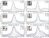 |
Fig. A.4 Same as Fig. A.1 for H ii region number 35 classified as filled. |
| In the text | |
Current usage metrics show cumulative count of Article Views (full-text article views including HTML views, PDF and ePub downloads, according to the available data) and Abstracts Views on Vision4Press platform.
Data correspond to usage on the plateform after 2015. The current usage metrics is available 48-96 hours after online publication and is updated daily on week days.
Initial download of the metrics may take a while.