| Issue |
A&A
Volume 552, April 2013
|
|
|---|---|---|
| Article Number | A56 | |
| Number of page(s) | 45 | |
| Section | Interstellar and circumstellar matter | |
| DOI | https://doi.org/10.1051/0004-6361/201219929 | |
| Published online | 25 March 2013 | |
OH far-infrared emission from low- and intermediate-mass protostars surveyed with Herschel-PACS⋆,⋆⋆
1
Institute for Astronomy, ETH Zurich, 8093
Zurich,
Switzerland
2
Centre for Star and Planet Formation, Natural History Museum of
Denmark, University of Copenhagen, Øster Voldgade 5–7, 1350
København K,
Denmark
e-mail: This email address is being protected from spambots. You need JavaScript enabled to view it.
3
Max Planck Institut für Extraterrestrische Physik,
Giessenbachstrasse 1,
85748
Garching,
Germany
4
Kavli Institute for Astronomy and Astrophysics at Peking
University, 100871
Beijing, PR
China
5
Leiden Observatory, Leiden University,
PO Box 9513, 2300 RA
Leiden, The
Netherlands
6
Centro de Astrobiología, CSIC-INTA, Carretera de Ajalvir, Km 4,
Torrejón de Ardoz, 28850
Madrid,
Spain
7
Department of Physics and Astronomy, Denison
University, Granville, OH,
43023,
USA
8
Department of Physics and Astronomy, University of
Waterloo, Waterloo,
Ontario, N2L 3G1, Canada
9
Université de Bordeaux, Laboratoire d’Astrophysique de Bordeaux,
CNRS/INSU, UMR 5804, Floirac, France
10
INAF – Osservatorio Astronomico di Roma,
00040
Monte Porzio Catone,
Italy
11
Department of Astronomy, Stockholm University,
AlbaNova, 106 91
Stockholm,
Sweden
Received:
1
July
2012
Accepted:
18
December
2012
Abstract
Context. The OH radical is a key species in the water chemistry network of star-forming regions, because its presence is tightly related to the formation and destruction of water. Previous studies of the OH far-infrared emission from low- and intermediate-mass protostars suggest that the OH emission mainly originates from shocked gas and not from the quiescent protostellar envelopes.
Aims. We aim to study the excitation of OH in embedded low- and intermediate-mass protostars, determine the influence of source parameters on the strength of the emission, investigate the spatial extent of the OH emission, and further constrain its origin.
Methods. This paper presents OH observations from 23 low- and intermediate-mass young stellar objects obtained with the PACS integral field spectrometer on-board Herschel in the context of the “Water In Star-forming regions with Herschel” (WISH) key program. Radiative transfer codes are used to model the OH excitation.
Results. Most low-mass sources have compact OH emission (≲5000 AU scale), whereas the OH lines in most intermediate-mass sources are extended over the whole 47.″0 × 47.″0 PACS detector field-of-view (≳20 000 AU). The strength of the OH emission is correlated with various source properties such as the bolometric luminosity and the envelope mass, but also with the [OI] and H2O emission. Rotational diagrams for sources with many OH lines show that the level populations of OH can be approximated by a Boltzmann distribution with an excitation temperature at around 70 K. Radiative transfer models of spherically symmetric envelopes cannot reproduce the OH emission fluxes nor their broad line widths, strongly suggesting an outflow origin. Slab excitation models indicate that the observed excitation temperature can either be reached if the OH molecules are exposed to a strong far-infrared continuum radiation field or if the gas temperature and density are sufficiently high. Using realistic source parameters and radiation fields, it is shown for the case of Ser SMM1 that radiative pumping plays an important role in transitions arising from upper level energies higher than 300 K. The compact emission in the low-mass sources and the required presence of a strong radiation field and/or a high density to excite the OH molecules points toward an origin in shocks in the inner envelope close to the protostar.
Key words: astrochemistry / stars: formation / ISM: molecules / ISM: jets and outflows
Herschel is an ESA space observatory with science instruments provided by European-led Principal Investigator consortia and with important participation from NASA.
Appendices are only available in electronic form at http://www.aanda.org
© ESO, 2013
1. Introduction
Oxygen is the most abundant element in the interstellar medium apart from hydrogen and helium. Many oxygen-bearing species, most importantly water and its precursors, have a very limited observability from the ground because of atmospheric constraints. The Herschel Space Observatory (Pilbratt et al. 2010) outperforms previous space-borne facilities in sensitivity as well as spatial and spectral resolution. It is thus well suited to study the water chemistry in young stellar objects (YSOs) in more detail. Because water undergoes large gas-phase abundance variations with varying temperature or radiation field, it is an excellent probe of the physical conditions and dynamics in star-forming regions (Kristensen et al. 2012; van Dishoeck et al. 2011).
A key connecting piece between atomic oxygen and water is the hydroxyl radical (OH). In the high-temperature gas-phase chemistry regime (T > 230 K), all available gas-phase oxygen is first driven into OH and then into water by the O + H2 → OH + H and subsequent OH + H2 → H2O + H reactions. The importance of the backward reaction H2O + H → OH + H2 depends on the atomic to molecular hydrogen ratio and therefore on the local UV field or shock velocity. H2 is dissociated in J-type shocks when the velocity exceeds ∼25 km s-1 (e.g. Hollenbach & McKee 1980). OH is also a byproduct of the H2O photo-dissociation process. Thus, OH is most abundant in regions with physical conditions different from those favoring the formation and existence of water and it therefore provides a complementary view of oxygen in the gas phase. In addition to its importance in the oxygen and water chemistry, OH also contributes to the FIR cooling budget of warm gas in embedded YSOs (e.g., Neufeld & Dalgarno 1989b; Kaufman & Neufeld 1996; Nisini et al. 2002; Karska et al. 2013). The goal of the “Water In Star-forming regions with Herschel” (WISH, van Dishoeck et al. 2011) Herschel key program is to study the H2O and associated OH chemistry for a comprehensive picture of H2O during protostellar evolution.
Detections of OH far-infrared (FIR) transitions from star-forming regions were made previously with the Kuiper Airborne Observatory (e.g. Melnick et al. 1987; Betz & Boreiko 1989), the Infrared Space Observatory (e.g. Ceccarelli et al. 1998; Giannini et al. 2001; Larsson et al. 2002; Goicoechea & Cernicharo 2002; Goicoechea et al. 2004, 2006), Herschel (e.g. van Kempen et al. 2010a; Wampfler et al. 2010, 2011; Goicoechea et al. 2011), and recently SOFIA (Csengeri et al. 2012; Wiesemeyer et al. 2012). Masers of OH hyperfine transitions are also commonly observed toward high-mass star-forming regions at cm wavelengths, but are not detected from low- and intermediate-mass protostars. Because this work focuses on low- and intermediate-mass YSOs, we will not discuss OH maser emission (a detailed overview can be found in e.g. Elitzur 1992).
From first Herschel results using the Photodetector Array Camera and Spectrometer (PACS, Poglitsch et al. 2010), van Kempen et al. (2010b) found that the OH emission from the low-mass class I YSO HH 46 is not spatially extended, in contrast to the H2O and high-J CO emission from the same source. They speculated that at least parts of the OH emission could stem from a dissociative shock caused by the impact of the wind or jet on the dense inner envelope. Spectrally resolved Herschel observations of OH with the Heterodyne Instrument for the Far-Infrared (HIFI, de Graauw et al. 2010) support an outflow scenario based on the inferred broad line widths of more than 10 km s-1 (Wampfler et al. 2010, 2011). Furthermore, analysis of OH PACS lines from a set of six low- and intermediate-mass protostars yielded similar excitation conditions of OH in all these sources (Wampfler et al. 2010). A tentative correlation of the OH line luminosities with the [OI] luminosities as well as the bolometric luminosities of the protostars were found, indicating that the observed OH emission might originate from a dissociative shock.
In this paper we present Herschel-PACS observations of OH in an extended sample of 23 low-and intermediate-mass YSOs. Our first goal is to test whether the tentative correlations from earlier work can be confirmed and to determine the influence of different source properties on the strength of the emission. The second goal is to study the OH excitation and the spatial extent of the OH emission in the target sources. A detailed analysis of the OH excitation and spatial extent is important to determine the origin of the OH emission and whether this is consistent with the picture from H2O observations.
The paper is organized as follows: Section 2 describes the source sample, the observations, and the data reduction methods. In Sect. 3 we present the observational results. Section 4 contains a discussion of spherically symmetric envelope models for OH (Sect. 4.1), the description and results of slab radiative transfer models to study the OH excitation in the outflow (Sect. 4.2), as well as the discussion and data interpretation (Sect. 4.3). Finally, the conclusions are summarized in Sect. 5.
Coordinates, distance, bolometric luminosity, and envelope masses of the low-mass class 0, class I, and intermediate-mass protostars in the sample.
Molecular data from the LAMDA database (Schöier et al. 2005) for the OH transitions detected with PACS.
2. Observations and data reduction
Observations of 23 low- and intermediate-mass YSOs were carried out with the Photodetector Array Camera and Spectrometer (PACS, Poglitsch et al. 2010) on the Herschel Space Observatory. All observations were obtained within WISH (van Dishoeck et al. 2011) except for IRAS 12496-7650 (DK Cha, van Kempen et al. 2010a), which was observed in the “Dust, Ice and Gas In Time” key program (DIGIT, PI N. Evans). The coordinates and properties of the targets can be found in Table 1 and the data identity numbers (obsids), observing modes, and the pipeline versions are given in Table A.1 in the appendix.
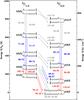 |
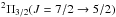
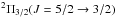
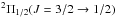
Fig. 1 OH transitions accessible with Herschel-PACS. Wavelengths are given in units of microns. Transitions that were observed for the entire source sample are shown in red. Transitions targeted only in the fraction of sources observed in range scan mode are depicted in blue if detected from at least one source and in gray if undetected. |
Two different observing modes are available for the PACS spectrometer, line and range
spectroscopy. The “range spectroscopy” mode provides a full scan of the
50−220 μm wavelength regime. The “line spectroscopy” mode covers only
small windows around selected target lines, but generally at higher spectral sampling and
sensitivity than range spectroscopy. The majority of the sources in our sample have been
observed with the PACS line spectroscopy mode, targeting four main OH rotational doublets:
 at 79 μm,
 at 84 μm,
 at 119 μm, and
 at 163 μm. The integration
time and the noise level for all sources observed in line spectroscopy mode is similar. NGC
1333 IRAS 4A and NGC 1333 IRAS 4B have been observed in both line and full range
spectroscopy. Range spectroscopy only was used for NGC 1333 IRAS 2A, Ser SMM 1, and DK Cha.
An illustration of the OH pure rotational transitions that are accessible with PACS on-board
Herschel is provided in Fig. 1. An
overview on the molecular data used in this work can be found in Table 2.
at 163 μm. The integration
time and the noise level for all sources observed in line spectroscopy mode is similar. NGC
1333 IRAS 4A and NGC 1333 IRAS 4B have been observed in both line and full range
spectroscopy. Range spectroscopy only was used for NGC 1333 IRAS 2A, Ser SMM 1, and DK Cha.
An illustration of the OH pure rotational transitions that are accessible with PACS on-board
Herschel is provided in Fig. 1. An
overview on the molecular data used in this work can be found in Table 2.
The full spectral scan of DK Cha was presented previously in van Kempen et al. (2010a) and the line spectroscopy of HH 46 and NGC 7129 FIRS 2 in van Kempen et al. (2010b) and Fich et al. (2010), respectively. These three spectra plus IRAS 15398, TMR 1, and NGC 1333 IRAS 2A were part of the sample analyzed in our previous work (Wampfler et al. 2010). We have now re-reduced all spectra with a newer version of the PACS pipeline and calibration files. The full spectral scans of NGC 1333 IRAS 4B and Ser SMM1 are discussed in great detail in Herczeg et al. (2012) and Goicoechea et al. (2012), respectively.
The PACS spectrometer is an integral field spectrometer and operates simultaneously in a
blue and a red channel. The detector consist of 5 by 5 square spatial pixels (“spaxels”)
with a pixel size of 9 4. The Herschel half power
beam width is smaller than a spaxel in the blue wavelength regime, but exceeds the spaxel
size on the sky in the red part of the spectrum. The spatial resolution is therefore limited
by the pixel size for short wavelengths and by the diffraction beam pattern at longer
wavelengths. The spectral resolution depends on the grating order and varies from
R = 3000−4000 at wavelengths
λ < 100 μm to
R = 1000−2000 for
λ > 100 μm. All individual OH lines
are therefore unresolved and at the lower resolutions, even blending of the OH doublets
occurs, mostly at 79 μm and 119 μm. When doublet
components are blended, they were assumed to be of equal strength in the analysis.
4. The Herschel half power
beam width is smaller than a spaxel in the blue wavelength regime, but exceeds the spaxel
size on the sky in the red part of the spectrum. The spatial resolution is therefore limited
by the pixel size for short wavelengths and by the diffraction beam pattern at longer
wavelengths. The spectral resolution depends on the grating order and varies from
R = 3000−4000 at wavelengths
λ < 100 μm to
R = 1000−2000 for
λ > 100 μm. All individual OH lines
are therefore unresolved and at the lower resolutions, even blending of the OH doublets
occurs, mostly at 79 μm and 119 μm. When doublet
components are blended, they were assumed to be of equal strength in the analysis.
The spectra were reduced with the Herschel interactive processing environment (HIPE, Ott 2010), versions 8 (for line scans) and 6 (for range scans). The wavelength grid was rebinned to four pixels per resolution element for line scans and two pixels per resolution element for range scans. The spectra were flat-fielded to improve the signal-to-noise ratio. The fluxes were normalized to the telescopic background and then calibrated using measurements of Neptune as a reference. The relative calibration uncertainty on the fluxes is currently estimated to be below 20%. The PACS spectrometer suffers from spectral leakage in the wavelength ranges 70−73 μm, 98−105 μm, and 190−220 μm where the next higher grating order ranges 52.5−54.5 μm, 65−70 μm, and 95−110 μm are superimposed on the spectrum. The fluxes from lines in these wavelength bands might therefore be less reliable than in parts of the spectra that are not affected by spectral leakage. This applies to the OH 71 μm and 98 μm doublets.
The lines were then subsequently analyzed in IDL using first or, if required, second order polynomials as baselines and the flux was measured by integrating over the line. The fraction of the point-spread function (PSF) seen by the central spaxel is wavelength-dependent, reaching from around 0.7 for a perfectly centered point source at 60−80 μm down to about 0.4 at 200 μm. A significant fraction of the flux might therefore fall onto neighboring spaxels and even more so if the source is off-centered on the central spaxel. It is therefore important to investigate the flux distribution on the detector, which can be caused by spatially extended emission, the telescope PSF, or a combination of both. Extracting the flux from all 25 spaxels is not an optimal solution, because of contamination from nearby sources and because the signal-to-noise ratio drops if many spaxels without line emission but extra noise are added. This is particularly problematic for weak lines or lines with little spatial extent. For a subset of our targets, where contamination from nearby sources occurs, we chose a set of spaxels that excludes the contribution from close-by sources. This applies to NGC 1333 IRAS 4A, NGC 1333 IRAS 4B, Ser SMM3, and DK Cha. Spaxels excluded in the flux measurements of the WISH sources are marked in gray in the maps in the online appendix B. For DK Cha, a 3 by 4 set around the on-source spaxel was used. For all other sources, we used either the on-source spaxel, corrected for the spillover (L 1527, Ced 110 IRS 4, L 723, L 1489, RNO 91), 3 by 3 spaxels centered on the on-source spaxel (IRAS 15398, L 483, TMR 1, TMC 1A, TMC 1, HH 46, and Ser SMM1), or the full array (all intermediate-mass sources).
3. Results and analysis
3.1. Detected lines and spatial extent
We detected at least one OH doublet in all 23 sources. The fluxes integrated over the
emitting area, obtained as described in Sect. 2, can
be found in Table 3. The doublet that is most often
detected, in 21 out of 23 sources, is the doublet at 84 μm, thanks
to a combination of intrinsic strength and higher spectral resolution of the instrument at
the shorter wavelengths. The component at 84.42 μm is however blended
with CO(31–30) at 84.41 μm because the spectral resolution is around
0.037 μm. The sources in which the 84 μm lines were
not detected are NGC 1333 IRAS 2A and AFGL 490. Figures 2 and 3 present the OH spectra of the
low-mass class 0 and class I sources, Fig. 4 the
spectra of the intermediate-mass sources. In 22 out of 23 sources at least one line was in
emission, with the exception being NGC 1333 IRAS 2A, where the only detection is the
119 μm doublet feature in absorption (Wampfler et al. 2010). We mainly detected emission lines, but absorption is also
found toward higher envelope masses. In the subsequent analysis, we only considered the
fluxes of lines that are purely in emission. Absorption in the 119 μm OH
 intra-ladder doublet transitions is
observed from NGC 1333 IRAS 2A and in some spaxels of AFGL 490, Vela IRS 17, and Vela IRS
19, but there are also spaxels with emission from these targets. For even higher envelope
masses like AFGL 490, the 79 μm OH cross-ladder transitions are also in
absorption. This behavior can be explained by the fact that both lines are directly
coupled to the ground rotational state of OH: because the first excited state is at
Eup ≈ 120 K, almost only the ground state is populated at
temperatures below ∼100 K. The 119 μm transitions couple the ground
state to the first excited state and have a large Einstein A coefficient
(∼1.4 × 10⁻¹ s-1). The 79 μm lines are
cross-ladder transitions between the ground states of both rotational ladders.
Cross-ladder transitions generally have much smaller Einstein A coefficients
(∼3.6 × 10⁻² s-1 for the 79 μm lines) than the
intra-ladder transitions. Therefore, absorption at 79 μm does not occur
as easily as for the 119 μm doublet.
intra-ladder doublet transitions is
observed from NGC 1333 IRAS 2A and in some spaxels of AFGL 490, Vela IRS 17, and Vela IRS
19, but there are also spaxels with emission from these targets. For even higher envelope
masses like AFGL 490, the 79 μm OH cross-ladder transitions are also in
absorption. This behavior can be explained by the fact that both lines are directly
coupled to the ground rotational state of OH: because the first excited state is at
Eup ≈ 120 K, almost only the ground state is populated at
temperatures below ∼100 K. The 119 μm transitions couple the ground
state to the first excited state and have a large Einstein A coefficient
(∼1.4 × 10⁻¹ s-1). The 79 μm lines are
cross-ladder transitions between the ground states of both rotational ladders.
Cross-ladder transitions generally have much smaller Einstein A coefficients
(∼3.6 × 10⁻² s-1 for the 79 μm lines) than the
intra-ladder transitions. Therefore, absorption at 79 μm does not occur
as easily as for the 119 μm doublet.
OH fluxes used throughout the paper in units of 10-16 W m-2 with 1σ errors from the flux extraction.
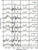 |
Fig. 2 PACS line scan OH spectra of the low-mass class 0 young stellar objects in our sample. The x-axis is wavelengths in μm, the y-axis is continuum subtracted flux density in Jy (plus a constant offset). The red dashed lines indicate the rest frequencies of the OH transitions. The blue dotted line represents the rest frequency of CO(31–30), which is blended with OH at 84.42 μm. The sampling of range scans (Ser SMM1 and NGC 1333 IRAS 2A) is different from line scans. |
Several sources show OH emission that is extended beyond what would be expected from a point source folded with the PSF of the telescope or leakage onto neighboring spaxels. The line emission is usually extended along the outflow direction (see Karska et al. 2013) and strongly correlated with the spatial extent of the atomic oxygen transitions, as illustrated in Fig. 5 and further discussed in Karska et al. (2013).
Maps of the OH 79, 84, 119, and 163 μm transitions for all WISH sources can be found in Appendix. An example of compact OH emission at 84 μm from the low-mass class I YSO L 1489 is shown in Fig. 6. Despite their location at further distances than the low-mass objects, all six intermediate-mass sources show signatures of extended OH emission. The largest spatial extent is seen in the 119 μm ground state lines, which can be excited most easily. Figure 7 presents the spaxel map of the 119 μm line from AFGL 490. The absorption is strongest toward the YSO and extended over an area of ∼25″ (25 000 AU) around the central position in the direction perpendicular to the outflow. The spatial extent of the emission is comparable to the 20 000 AU by 6000 AU envelope structure discussed in Schreyer et al. (2006). The OH absorption changes into weak emission along the outflow direction. For the full sample we provide an overview whether the flux observed outside the on-source spaxel is consistent or inconsistent with the spillover factor in Table 4.
3.2. OH emission line flux ratios
Comparison of the OH 84 μm line luminosities (flux corrected for the source distance) between the different source types shows that the intermediate-mass sources in our sample have higher OH luminosities than the low-mass sources by about two orders of magnitude on average. Among the low-mass sources, the class 0 sources are on average about a factor of two more luminous in OH than the class I sources.
In earlier work (Wampfler et al. 2010), we found that the line flux ratios among the sources in the sample were relatively constant. We have therefore also calculated the 79 μm / 84 μm, 79 μm / 119 μm, 79 μm / 163 μm, 84 μm / 119 μm, 84 μm / 163 μm, and 119 μm / 163 μm line flux ratios for the extended sample, i.e. the sources in Table 1 from which emission was detected. The fluxes of doublets are added except for the 84 μm doublet, because the 84.42 μm is blended with CO(31–30). Instead we use twice the flux of the 84.60 μm component assuming that both components are of similar strength. Cases where only one doublet component was clearly detected were not considered. The results are listed in Table 5.
Again we find that the line ratios remain relatively constant within less than a factor of four around their mean values over the whole luminosity, mass, and age range of several orders of magnitude spanned by the sample. The excitation of OH is therefore likely to be similar in all sources, indicating that either the OH emission stems from gas at similar physical conditions or that the ratios remain stable over a spread of parameter values. The latter possibility is supported by the models (cf. Sect. 4), but does not exclude the first option.
3.3. OH rotational temperature
The full spectral scans cover the OH transitions from about 55−200 μm
(Eup ≈ 120−875 K) and therefore allow us to study the
excitation conditions by means of rotational diagrams. Figure 8 presents the diagram for Ser SMM1. The derived rotational temperature
is Trot ≈ 72 ± 8 K if all the transitions shown on the plot
except the 119 μm (optically thick), 84.42 μm (blended
with CO), and 98 μm (in leaking region) are included. The rotational
diagram for NGC 1333 IRAS 4B can be found in Herczeg
et al. (2012), giving Trot ≈ 60 ± 15 K. No emission
lines were detected in the full spectral scan of NGC 1333 IRAS 2A and only very few line
detections are available for NGC 1333 IRAS 4A and DK Cha (see also van Kempen et al. 2010a), so that the rotational diagram for these
sources is very sparsely populated and a fit of the rotational temperature is therefore
not feasible. For Ser SMM1, the corresponding OH column density would be
NOH = 1.0 × 1014 cm-2 assuming a
source size of 20″ and using an interpolated value for the partition function
Q from the JPL catalog1 (Pickett et al. 1998). However, the
 points fall below the fit, suggesting that
these transitions are either optically thick, which is well possible because the
ladder contains the ground rotational
state, or that the two rotational ladders might have a different rotational temperature.
points fall below the fit, suggesting that
these transitions are either optically thick, which is well possible because the
ladder contains the ground rotational
state, or that the two rotational ladders might have a different rotational temperature.
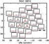 |
Fig. 5 Map of the OH 84 μm (red) and [OI] 63 μm emission (black) from NGC 2071, illustrating the similar spatial extent of the two transitions. The x-axis is velocity in km s-1, the y-axis continuum subtracted and normalized flux density. All spaxels were normalized with respect to the spaxel that contains the peak of the continuum emission at 63 μm. Note that the peak of the continuum emission at 84 μm falls onto the central spaxel, although the two observations were carried out consecutively. |
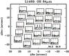 |
Fig. 6 Map of the compact OH 84 μm emission from L 1489. The x-axis is wavelength in μm, the y-axis continuum subtracted and normalized flux density. All spaxels were normalized with respect to the central one. The red dashed lines indicate the rest frequencies of the OH transitions, the blue dashed line the CO(31–30). |
Description whether the fluxes measured in the on-source spaxel and the surrounding three by three spaxels are consistent with the pure spillover factor (0.70 at 79 μm, 0.69 at 84 μm, 0.62 at 119 μm, and 0.49 at 163 μm).
3.4. Dependence of OH luminosity on source properties
Understanding which source parameters influence or even determine the strength of the OH emission and the excitation of the different transitions is important to constrain the origin of the emission. We therefore test whether the OH line luminosity correlates with various envelope parameters and the emission from other molecular and atomic species. Because the different OH transitions are fairly well correlated (Sect. 3.2), we restrict the analysis to the 84 μm luminosity, where we have most detections.
In Figs. 9 and 10 the dependence of the OH line luminosity on the bolometric source luminosity and the envelope mass are shown, respectively. We use new values for Lbol that were derived by Kristensen et al. (2012) based on additional continuum values from PACS observations, which are presented in Karska et al. (2013). The envelope masses for the low-mass sources are calculated from spherical models based on continuum radiative transfer and include all material at temperatures above 10 K. For the intermediate-mass sources, we use literature values and the method that was used to determine the envelope mass may therefore be different.
The Pearson correlation coefficient, defined as
ρX,Y = cov(X,Y) / [σ(X) × σ(Y)],
i.e. the covariance of two random variables X and Y
divided by their standard deviations, for LOH with
Lbol is 0.93, including all 21 sources where the OH
84 μm line was detected. An overview on all obtained correlation
coefficients and their corresponding significance levels is given in Table 6. Values of ρ close to 1 and − 1
describe a tight correlation or anticorrelation of the parameters X and
Y, respectively, while values close to 0 indicate that
X and Y are uncorrelated. At what level of
ρ a correlation is considered to be significant, depends on the number
of data points. The significance of ρ can be expressed as a probability
value, the significance level p, and tells how likely the actual observed
or a more extreme value of ρ is found under the assumption that the null
hypothesis is true, i.e. that there is no relationship between the parameters. Another
option is to express the significance in terms of number of standard deviations
σ, calculated from  , where N is the number of
sources.
, where N is the number of
sources.
The correlation coefficient for LOH with
Menv is smaller (ρ = 0.84). As illustrated
by Fig. 11, the bolometric luminosity and the
envelope mass are not independent properties of the sources. This is consistent with Bontemps et al. (1996, Fig. 1) and André et al. (2000, Fig. 6b), who found that
Lbol and Menv are strongly
correlated for the class 0 sources and that class I sources move down in the diagram with
time along the evolutionary tracks. From an
LOH − Menv correlation one would
also expect LOH to be correlated with
Tbol (Fig. 8 of Jørgensen
et al. 2002). Such a correlation is however not found for our low-mass source
sample, as illustrated by Fig. 12, indicating that
the underlying Lbol − Menv
correlation might create the observed
LOH − Menv trend. A correlation
between two variables can be caused by an underlying correlation of the two variables with
a third one. A method to measure such effects is the concept of the partial correlation
coefficient, defined as  (see also Appendix A from Marseille et al. 2010). The resulting value for the
partial correlation coefficient of LOH with
Menv under the influence of Lbol
is 0.56, i.e. significantly reduced, thus indicating that the trend might indeed be based
on an underlying relation between mass and luminosity. Class I YSOs that lie above the
LOH − Menv correlation in Fig.
10 are also the ones that do not follow the
Lbol − Menv relation (Fig. 10), in particular DK Cha. These sources have a higher
LOH than what would be expected from their mass and a lower
value than what would be expected from their bolometric luminosity. They are found in the
region of more evolved class I sources (see Fig. 6 in André
et al. 2000), i.e. they have a significantly lower envelope mass at a given
bolometric luminosity than less evolved sources like e.g. HH 46, and are in the
transitional stage to class II where disk emission may contribute as well.
(see also Appendix A from Marseille et al. 2010). The resulting value for the
partial correlation coefficient of LOH with
Menv under the influence of Lbol
is 0.56, i.e. significantly reduced, thus indicating that the trend might indeed be based
on an underlying relation between mass and luminosity. Class I YSOs that lie above the
LOH − Menv correlation in Fig.
10 are also the ones that do not follow the
Lbol − Menv relation (Fig. 10), in particular DK Cha. These sources have a higher
LOH than what would be expected from their mass and a lower
value than what would be expected from their bolometric luminosity. They are found in the
region of more evolved class I sources (see Fig. 6 in André
et al. 2000), i.e. they have a significantly lower envelope mass at a given
bolometric luminosity than less evolved sources like e.g. HH 46, and are in the
transitional stage to class II where disk emission may contribute as well.
Observed line flux ratios (see text for details).
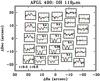 |
Fig. 7 Map of spatially extended OH 119 μm absorption and emission from AFGL 490. The x-axis is wavelength in μm, the y-axis continuum subtracted and scaled flux density. The labels indicate the multiplicative scaling factors for each spaxel unless they are unity. |
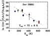 |
Fig. 8 Rotational diagram for the OH lines measured from Ser SMM1. Transitions belonging
to the |

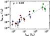 |
Fig. 9 OH luminosity of the 84 μm transition vs. bolometric luminosity of the source. Low-mass class 0 sources are shown as red diamonds, class I sources as blue triangles, and intermediate-mass protostars as green circles with 3σ error bars from the flux determination (does not include the calibration uncertainty). The dashed line is a linear fit to the data. |
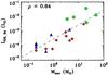 |
Fig. 10 OH 84 μm luminosity vs. envelope mass of the source. |
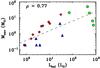 |
Fig. 11 Bolometric luminosity vs. envelope mass of the sources. |
Pearson’s correlation coefficients ρ, number of sources N, corresponding significance levels p, and number of standard deviations σ for the OH 84.6 μm line luminosity or flux and various envelope parameters.
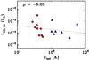 |
Fig. 12 OH 84 μm luminosity vs. bolometric temperature of the sources. |
We find that LOH (the luminosity of the OH 84 μm transitions) seems to be well correlated with luminosity for both evolutionary stages and that class 0 and I sources lie on the same straight line. In contrast, Nisini et al. (2002) found from ISO data that class I sources fall systematically below class 0 sources in their plot of the total FIR luminosity LFIR = L[OI] + LCO + LH2O + LOH versus Lbol. Furthermore, they concluded that class 0 and I sources fall onto the same straight line in the LFIR − Menv plot, but in Fig. 6 of Nisini et al. (2002), class I sources with Menv ≲ 10-1 L⊙ tend to branch off as well.
A correlation of LOH with the outflow momentum flux (“outflow force”, Bontemps et al. 1996) FCO is not significant from our Fig. 13. The values for FCO are taken from the literature and were not derived in a consistent way. New estimates of FCO are currently work in progress (Yıldız et al., in prep.).
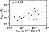 |
Fig. 13 OH 84 μm luminosity vs. outflow force. |
Furthermore, LOH seems to decrease with evolution for class 0
sources, but not for class I, as can be seen from Fig. 14 showing LOH plotted against
 , a quantity that was proposed as an
evolutionary tracer by Bontemps et al. (1996).
, a quantity that was proposed as an
evolutionary tracer by Bontemps et al. (1996).
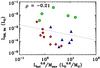 |
Fig. 14 OH 84 μm luminosity vs. luminosity to the 0.6 divided by the envelope mass of the sources (evolutionary tracer). |
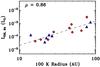 |
Fig. 15 Correlation of OH 84 μm luminosity with the 100 K radius of the spherical source models. |
The different behavior of the class 0 and I sources could be caused by their different geometry. If the OH was radiatively pumped, then the location of the warm dust would be an important parameter. Warm dust at 100 K (cf. Sect. 3.3) is expected from two physical components in YSOs, the inner envelope and the outflow walls. Class 0 and class I sources differ in the geometrical alignment of their warm dust components: in class 0 sources, high-energetic radiation from the protostar and accretion processes is reprocessed to a FIR field by the dust in the inner envelope, which represents a small solid angle. Thus the OH luminosity for sources where this component dominates should be mass dependent. In class I sources, the warm dust from the outflow walls can directly irradiate the local OH molecules and therefore the OH luminosity for these sources should depend on the bolometric luminosity. We extracted the radius at which the temperature reaches 100 K from the spherically symmetric envelope models to test this hypothesis. Figure 15 shows the OH luminosity plotted against the 100 K radius from the spherically symmetric envelope models (Kristensen et al. 2012) and there seems to be a trend of increasing OH luminosity when the size of the inner hot envelope T ≥ 100 K is larger. The OH luminosity does not seem to depend significantly on the density at 1000 AU as shown in Fig. 16. A correlation with density would not necessarily imply that collisions are the dominant excitation mechanism anyway as the dust mass also increases with density.
3.5. Correlation of the OH flux with other species
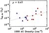 |
Fig. 16 Correlation of OH 84 μm luminosity with the H2 density at 1000 AU from the spherical source models. |
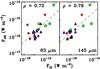 |
Fig. 17 Correlation of OH 84 μm and [OI] 63 μm and 145 μm fluxes. |
OH is tightly related to the formation and destruction processes of H2O and a
connecting piece between H2O and atomic oxygen in the chemistry. We therefore
test whether the OH emission is correlated with the [OI] and H2O emission. The
[OI] and H2O fluxes for the low-mass protostars are tabulated in Karska et al. (2013) and those of the intermediate-mass
protostars in Table A.2 in the appendix. Figure
17 shows the OH 84 μm flux
plotted versus the [OI]  P
P P2 and
P
P2 and
P P1 fluxes at
63 μm (left panel) and 145 μm (right panel),
respectively. The Pearson correlation coefficients for OH 84 μm vs. [OI]
63 μm and 145 μm are 0.72 and 0.79, respectively,
corresponding to a three sigma result. The [OI] 63 μm could be optically
thick or more affected by contamination than the 145 μm, which would
explain the slightly lower correlation coefficient for OH 84 μm vs. [OI]
63 μm compared to [OI] 145 μm. The OH and [OI]
emission thus seem to be correlated both spatially and in total flux, hinting at a common
origin, most likely from gas associated with the outflow, because in the cases of
noncompact emission it is usually found to be extended along the outflow direction.
P1 fluxes at
63 μm (left panel) and 145 μm (right panel),
respectively. The Pearson correlation coefficients for OH 84 μm vs. [OI]
63 μm and 145 μm are 0.72 and 0.79, respectively,
corresponding to a three sigma result. The [OI] 63 μm could be optically
thick or more affected by contamination than the 145 μm, which would
explain the slightly lower correlation coefficient for OH 84 μm vs. [OI]
63 μm compared to [OI] 145 μm. The OH and [OI]
emission thus seem to be correlated both spatially and in total flux, hinting at a common
origin, most likely from gas associated with the outflow, because in the cases of
noncompact emission it is usually found to be extended along the outflow direction.
The correlation of the OH 84 μm flux with p-H2O 32, 2 − 21, 1 (λ ≈ 89.99 μm, Eup = 296.8 K) is shown in Fig. 18. The p–H2O 32, 2 − 21, 1 was chosen because it has a very similar upper level energy to the OH 84 μm transition (Eup = 290.5 K) and a similar wavelength, which strongly reduces the influence of instrumental effects, as the PSF is very similar. The fluxes were measured on the same spaxel sets. The correlation of the OH 84 μm flux with p–H2O 32, 2 − 21, 1 is significant at more than 3σ with ρ = 0.85. The same plot for o–H2O 21, 2 − 10, 1 (λ ≈ 179.53 μm, Eup = 114.4 K) can be found in Karska et al. (2013). The o–H2O 21, 2 − 10, 1 line has a lower upper level energy and was observed in a larger beam, but was detected in more sources. Again, there is a statistical correlation between the fluxes of the OH and H2O lines at similar energy, but the H2O and OH spatial extents can differ (Karska et al. 2013).
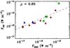 |
Fig. 18 Correlation of OH 84 μm and H2O 89.99 μm fluxes. |
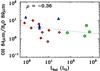 |
Fig. 19 OH 84 μm flux divided by H2O 89 μm flux vs. bolometric luminosity of the sources. Low-mass class I sources have a higher ratio than class 0 sources on average. |
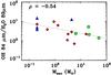 |
Fig. 20 OH 84 μm flux divided by H2O 89 μm flux vs. envelope mass of the sources. |
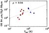 |
Fig. 21 OH 84 μm flux divided by H2O 89 μm flux vs. bolometric temperature of the sources. |
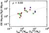 |
Fig. 22 OH 84 μm flux divided by H2O 89 μm flux vs. evolutionary tracer. |
The ratio of the two fluxes versus the bolometric luminosity is shown in Fig. 19. The low-mass class I sources lie in the upper part of the plot as they have OH 84 μm to H2O 89 μm ratios above 2–3, whereas the class 0 sources have a slightly lower ratio on average. On the other hand, there is no significant trend with bolometric luminosity (ρ = −0.36). The ratio seems to decrease with envelope mass, as illustrated by Fig. 20, and to increase with bolometric temperature (Fig. 21), but there is a large spread. Figure 22 shows that an increase in the OH 84 μm to H2O 89 μm ratio could be an evolutionary effect. The increase in OH compared to H2O could for instance be caused by the envelope becoming more tenuous in the more evolved stages, allowing high-energy photons from the protostar to penetrate further and dissociate the H2O. The intermediate-mass sources are missing in Fig. 21, because a consistent set of bolometric temperatures is not available.
Goicoechea et al. (2011) find that the OH 84 μm emission is not spatially correlated with o–H2O 30, 3 − 21, 2 in the Orion Bar PDR, but with high-J CO and CH+. We cannot test such a spatial correlation here because the fluxes drop rapidly outside the on-source spaxels in our low-mass source sample.
4. Excitation and origin of OH
Where does the OH emission arise? The environment of low-mass protostars is known to consist of different physical components, including the collapsing envelope, shocks, outflow cavities heated by UV radiation, and entrained outflow gas, all of which are contained in the Herschel beams (see Visser et al. 2012, for an overview). To derive physical properties like the density and temperature of the emitting gas, the observed fluxes and line ratios are compared to the results from radiative transfer models. The obtained physical conditions can help in constraining the origin of the emission in combination with information about the spatial distribution of the emission. Furthermore, radiative transfer models permit to study what mechanism dominates the excitation under given physical conditions.
The lowest rotational transitions of OH lie in the FIR and therefore significantly interact with the dust continuum field, which peaks in the same wavelength regime for dust temperatures typical of embedded YSOs. Moreover, the properties of OH such as the large dipole moment and large rotational constant make radiative pumping an important excitation process. Therefore, the excitation of OH should be modeled using a code that includes radiative effects.
Before describing the models, we recall the clues on the origin of the OH emission that come from spectrally resolved OH line profiles. Wampfler et al. (2010) present upper limits on the OH 163 μm (1837 GHz) line intensities using HIFI for two low-mass sources which, when combined with measured PACS fluxes for the same lines, imply FWHM line widths of at least 10 km s-1. For a third low-mass source, Ser SMM1, a recent unpublished HIFI spectrum shows a detection of the broad (FWHM ≈ 20 km s-1) component, but no sign of a narrow component (Wampfler et al., in prep.). In contrast, Wampfler et al. (2011) found a narrow component (FWHM ≈ 4−5 km s-1) in the OH 1837 GHz spectrum from the high-mass protostar W3 IRS 5, which can be attributed to the quiescent envelope, on top of a broad outflow component with FWHM ≈ 20 km s-1. Therefore, the OH line profiles from low-mass YSOs seem to be dominated by the outflow contribution, whereas those of high-mass sources can contain both an outflow and envelope component.
4.1. Spherical envelope models
To further quantify any contribution from the protostellar envelope, spherically symmetric source models such as derived by Kristensen et al. (2012) are commonly used in combination with a nonLTE line radiative transfer code like RATRAN (Hogerheijde & van der Tak 2000) or LIME (Brinch & Hogerheijde 2010) to model the line emission.
We ran RATRAN calculations in spherical symmetry for a few low-mass sources, including Ser SMM1, using the same RATRAN code as for W3 IRS 5 (see Sect. 4.2.1 for molecular data input). The OH fractional abundances considered range from xOH = 10-9 to 10-7. Note that the source structure on small scales is often not well constrained by the single-dish continuum observations and that the spherical symmetry starts to break down inside about 500 AU (e.g. Jørgensen et al. 2005). Thus this type of model is not ideally suited for lines with a high critical density, where the bulk of the emission usually arises from the innermost parts of low-mass protostellar envelopes. The inner envelope is also the area where the excited states of OH are mainly populated, and thus the model results should only be regarded as a rough order of magnitude estimate.
It is clear that these spherically symmetric source models cannot reproduce the observed OH emission in low-mass sources for a variety of reasons. First, the synthetic spectra from the model fail to reproduce the observed broad lines (FWHM of ∼20 km s-1). The model lines are typically much narrower (FWHM of a few km s-1) for any reasonable Doppler− b parameter that fits emission from other molecules. Therefore, the line width measured from the HIFI spectra is inconsistent with an envelope-only or envelope-dominated scenario for the low-mass sources observed with HIFI. Moreover, the 79, 84, and 119 μm lines from the RATRAN models are always in absorption, while the detected PACS lines from the low-mass sources are in emission, providing another indication that the bulk of the emission does not arise from the envelope. Although a minor envelope contribution to the 163 μm lines cannot be excluded, the bulk of the emission is likely associated with the outflow. For the intermediate-mass sources, absorption is observed at 119 μm in at least one spaxel (except for NGC 7129 FIRS 2), suggesting that a potential envelope contribution to the spectra of intermediate-mass sources cannot be excluded, in particular in the lowest rotational transitions.
4.2. Outflow model
4.2.1. Slab model description
To model OH emission from outflows or shocks, a simple slab geometry is appropriate. We
use a radiative transfer code based on the escape probability formalism as described in
Takahashi et al. (1983), which includes
radiative pumping. The physical conditions such as density and temperature and the
excitation of the molecule are assumed to be constant throughout the region. The free
parameters of the model are the kinetic temperature of the gas
Tgas, the temperature of the dust
Tdust, the density of the collision partner
n, the molecular column density of OH
NOH, and the dust column density
Ndust. The line profile function has a rectangular shape
with a width of 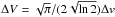 where Δv is the full
width at half maximum (FWHM) of a Gaussian line. Here, Δv is assumed to
be 10 km s-1 for all models. As discussed above, this FWHM is motivated by
the nondetection of OH from low-mass sources with HIFI (Wampfler et al. 2010) that lead to the conclusion that the line width must be
broader than 10 km s-1.
where Δv is the full
width at half maximum (FWHM) of a Gaussian line. Here, Δv is assumed to
be 10 km s-1 for all models. As discussed above, this FWHM is motivated by
the nondetection of OH from low-mass sources with HIFI (Wampfler et al. 2010) that lead to the conclusion that the line width must be
broader than 10 km s-1.
Our slab code is similar to the “RADEX” code (van der Tak et al. 2007), but includes an active dust continuum, which is capable of both absorbing and emitting radiation. Results from our code in the limiting case where no dust is present agree very well with the RADEX results. An earlier OH excitation study by Offer & van Dishoeck (1992) included a dust continuum radiation field for the radiative excitation but not the absorption of line photons by dust grains. Furthermore, different dust properties were used in their calculations. Therefore, the comparability of the two models is limited.
We use the molecular data file from the Leiden atomic and molecular database (LAMDA,
Schöier et al. 2005) for OH without hyperfine
structure, because the resolution of PACS does not allow one to resolve the hyperfine
components. The file contains frequencies, energy levels, and Einstein A coefficients
from the JPL catalog (Pickett et al. 1998) and
collision rates with ortho- and para-H2 for temperatures in the range of
15−300 K from Offer et al. (1994). The highest
excited state contained in the file has an energy of 875 K. The
ortho-to-para-H2 ratio in the model is temperature dependent according to
![Mathematical equation: \begin{equation} r = \min \left[3.0, 9.0 \times \exp \left( \frac{-170.6}{T}\right) \right]\cdot \end{equation}](/articles/aa/full_html/2013/04/aa19929-12/aa19929-12-eq294.png) (1)The dust opacities for dust grains with
thin ice mantles in the wavelength range of 1−1300 μm are taken from
Ossenkopf & Henning (1994,Table 1, Col. 5).
(1)The dust opacities for dust grains with
thin ice mantles in the wavelength range of 1−1300 μm are taken from
Ossenkopf & Henning (1994,Table 1, Col. 5).
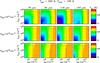 |
Fig. 23 Excitation temperature from slab models with Tgas = 200 K and Tdust = 100 K for the OH lines at 79, 84, 119, and 163 μm for OH column densities of 1014, 1016, and 1018 cm-2, and varying H2 density and dust column density. The dashed line indicates the critical density of the upper level of each transition, the dotted line marks where the dust becomes optically thick. |
The parameter space explored in the slab models covers the full range of physical conditions expected in the protostellar environment, i.e., temperature range T = 50−800 K, densities of n = 104−1012 cm-3, dust column densities of NOH = 1018−1023 cm-2, and OH molecular column densities of 1014−1018 cm-2. Temperatures above 800 K are problematic because the highest rotational level included in the molecular data file is 875 K and the collision rates are only available up to 300 K. The collisional de-excitation rates are kept constant above 300 K, and the excitation rates are calculated from the de-excitation rates from the detailed balance relations and thus depend on the kinetic temperature through a factor exp[−ΔE / kBTkin].
4.2.2. Slab model results
A useful quantity to describe the excitation of a molecule is the excitation
temperature, defined as 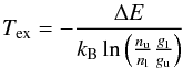 (2)where gl and
gu are the statistical weights of the lower and upper
level, respectively, and nl and
nu their normalized populations. The energy of the
transition is ΔE = hν and
kB denotes Boltzmann’s constant.
(2)where gl and
gu are the statistical weights of the lower and upper
level, respectively, and nl and
nu their normalized populations. The energy of the
transition is ΔE = hν and
kB denotes Boltzmann’s constant.
Figure 23 shows the excitation temperature of the OH transitions at 79.18 μm, 84.60 μm, 119.44 μm, and 163.12 μm as a function of nH2 and Ndust for a model of fixed gas and dust temperatures (Tgas = 200 K, Tdust = 100 K) and three values of NOH. The NOH = 1014 cm-2 model largely represents the optically thin case, the NOH = 1018 cm-2 model the optically thick regime, and NOH = 1016 cm-2 is an intermediate case. The adopted parameters are representative for the OH emitting region.
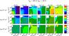 |
Fig. 24 Line flux ratios from slab models with Tgas = 200 K and Tdust = 100 K for the OH lines at 79, 84, 119, and 163 μm for OH column densities of 1014, 1016, and 1018 cm-2, and varying H2 density and dust column density. The shaded area marks the observed values. |
We notice from Fig. 23 that all transitions behave relatively similar with respect to their excitation. Furthermore, this behavior is also comparable for all considered gas temperatures (50, 100, 200, 500, and 800 K). For densities above the critical density (∼108 cm-3), the excitation temperature approaches the kinetic temperature of the gas, as expected, irrespective of the dust column density. The populations are thermalized at the kinetic temperature. Collisions must therefore be the dominant excitation mechanism in this regime. For densities below the critical density, dust pumping dominates the excitation for dust column densities above ∼1021 cm-2. This is illustrated by the fact that Tex approaches Tdust, i.e. the populations are thermalized at the temperature of the dust radiation field. Below Ndust ≈ 1021 cm-2, both mechanisms contribute to the excitation, whereby one order of magnitude increase in nH2 and Ndust have similar effects on Tex. If the OH column density is enhanced, the gas becomes optically thick and line photons are trapped. Then, the level populations thermalize at the gas temperature already at lower densities because the critical density is reduced with an effective critical density of ncr(τline) ≈ ncr(0) / τline.
In models of equal dust and gas temperature, we find that the 79 μm cross-ladder transition even experiences supra-thermal excitation for low densities (nH2 ≲ 108 cm-3), temperatures above 50 K, OH column densities 1014−1016 cm-2, and dust column densities in the range of 2 × 10²⁰−1 × 1022 cm-2.
As for line optical depths, the models show that the 119 μm
transition reaches the highest optical depth as expected from the fact that this
transition is connected to the ground state. It is followed by the
84 μm transition, originating from the same rotational ladder, just
above the 119 μm. The 79 μm line is a cross-ladder
transition with a much smaller Einstein A coefficient and does therefore not become
optically thick as easily as the two afore mentioned
intra ladder transitions.
Figure 24 presents the line flux ratios for the six possible combinations of the observed four transitions. We decided to use line ratios instead of fluxes because the ratios are less dependent on the source size. The black contours represent the minimum and maximum value of the observed ratios and the shaded area indicates where the models match the observed values, given in Table 5. White areas at high dust column densities indicate regions where at least one line is in absorption. The observed line ratios can be modeled with a wide range of parameters, but the observed line ratios still allow us to exclude parts of the parameter space. The very optically thin model (NOH = 1014 cm-2) fails to reproduce the observed 79 μm / 119 μm line flux ratio for temperatures below 200−500 K and can also hardly match the 119 μm / 163 μm ratio. Similar difficulties occur for the very optically thick case (NOH = 1018 cm-2), where the observed 79 μm / 163 μm ratio can only be found in a very narrow range of dust column densities. A direct comparison of the column density with observations is however difficult because the model does not include any geometrical effects.
There are basically two main regimes in the intermediate case (NOH = 1016 cm-2) that are able to reproduce to the observed values. First, there is the radiatively dominated regime at low densities (104−108 cm-3) for dust column densities in the range of Ndust ≈ 1 × 10¹⁹−3 × 1021 cm-2, slightly depending on temperature (lower Ndust for higher temperature and vice versa). In the regime where collisions start to become important (n ≳ 106 cm-3) and at low dust column densities (Ndust ≲ 1020 cm-2), it is harder to find a set of parameters that is able to reproduce all line ratios simultaneously, in particular the 79 μm / 84 μm, 79 μm / 163 μm, and 84 μm / 163 μm ratios. For densities of 106−108 cm-3, small ranges can however be found, especially given the uncertainties of our line ratios. At temperatures below ∼100 K, a collision dominated solution exists toward higher densities (n ≳ 108 cm-3) and dust column densities above ∼3 × 1020 cm-2. So given the degeneracies in the models, we cannot well distinguish between collisional excitation and radiative pumping unless we have additional constraints on the density of the emitting gas and the dust column density.
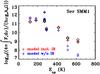 |
Fig. 25 Comparison of the rotational diagram for the OH lines measured from Ser SMM1 (black diamonds) and a RADEX model with the source continuum included in the excitation (red plus signs) and a model without the continuum field of the source (blue plus signs). The model fluxes were scaled such that they match the observed 84.60 μm emission. The model including the continuum field reproduces the higher excited lines better than the one without. |
To constrain which of the two scenarios is more likely, we ran additional RADEX slab models (van der Tak et al. 2007) that allow us to include the actual continuum field of a source at a given distance. The line width is chosen to be 10 km s-1 and the density and temperature at a given distance are taken from the continuum model of the source presented in Kristensen et al. (2012). The OH column density is a free parameter. The continuum field is only included in the excitation of the OH molecules, but not in the line formation, thus assuming a geometry in which the OH is not right in front of the line of sight to the continuum. Models which include the source continuum in both the excitation and the line formation yield several lines in absorption and cannot reproduce the observations. To study the importance of the continuum, models without the continuum field were calculated as well. The model fluxes were scaled such that the 84.60 μm flux is equal to the observed value.
Figure 25 shows the results for Ser SMM1 (n = 8 × 107 cm-3 and T = 90.3 K at a distance of 100 AU) and NOH = 1016 cm-2. While the modeled fluxes are fairly similar for the transitions with an upper level energy less than 300 K, the model including the continuum field matches the observed values better than that without a source continuum for the higher excited lines (98 μm, 65 μm, and 71 μm).
Another indication that the continuum may be important is illustrated by Fig. 26 showing the correlation of the OH 84 μm flux with the continuum at 63 μm and 84 μm as measured from the PACS data. A continuum field with a temperature similar to the observed rotational temperature of OH, i.e. Trad ≈ 100 K, would peak at around 30 μm, which cannot be observed with Herschel. Therefore, we use the continuum at 63 μm and 84 μm instead.
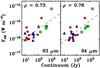 |
Fig. 26 Correlation of OH 84 μm flux with the continuum fluxes measured from the PACS data at 63 μm and 84 μm. |
For the Orion bar, Goicoechea et al. (2011) found line ratios that differ from the values derived for our source sample, except for the 79 μm / 119 μm and 79 μm / 163 μm ratios. The 79 μm / 84 μm ratio of almost four is higher than in our sample, as is the 119 μm / 163 μm ratio. On the other hand, the 84 μm / 119 μm and 84 μm / 163 μm ratios are lower. The temperature, density, and the column density of the dust grains are lower in the Orion bar, therefore both collisional excitation and pumping by the FIR field are likely lower.
4.3. Discussion
From the PACS observations we find that the excitation of the OH emission in our sample of 17 low- and 6 intermediate-mass protostars is similar in all sources, as indicated by the relatively constant line ratios among the target sample. This could either mean that the OH emission from all sources arises from gas at very similar physical conditions or that the observed line ratios can be realized by a broad range of gas properties. Comparison of the ratios to the modeling results (cf. Sect. 4.2.2) shows that the observed values can indeed be reproduced by a wide parameter range, which may explain why similar ratios are observed in sources that span a large range in luminosity, envelope mass, and evolutionary stage.
From the full range scans of the two class 0 YSOs Ser SMM1 and NGC 1333 IRAS 4B we find that the rotational temperature of OH in these sources is around 70 K. From the fact that the points can be relatively well fitted with a straight line in the rotational diagram, we conclude that the level population of OH can be represented by a Boltzmann distribution at T ≈ 70 K. The constant line ratios found in the sample may be an indication that other sources could have similar rotational temperatures. However, the models demonstrate that different physical conditions are able to reproduce the observed line ratios and thus full range scan data, which includes more than four OH transitions, of additional sources is needed to test how the OH rotational temperatures vary from source to source and whether there is any difference between evolutionary stages. If the rotational temperature were equal to the ambient kinetic temperature, the population would be in LTE. However, because of the very high critical densities of most OH transitions (around 108 cm-3), this scenario seems to be rather unlikely, as a significant amount of the emission stems from the outflow (Wampfler et al. 2010, 2011). Compression factors of a hundred are needed to obtain a post-shock density of 108 cm-3 for a pre-shock density of 106 cm-3 (Neufeld & Dalgarno 1989a). Alternatively, the OH excitation may be in equilibrium with the temperature of the FIR dust continuum field, that can strongly pump OH.
The models show that the degeneracy in the parameter space is large, allowing different combinations of parameters for the realization of the observational results. Therefore, it is only possible to distinguish between the collision-dominated and radiative pumping controlled scenarios described in Sect. 4.2.2 when additional constraints on the density and dust column density of gas emitting or absorbing in OH FIR lines are available. The similar line ratios could be a hint that the excitation is not controlled by a combination of both collisions and radiative pumping but rather by one dominant mechanism, because it would be much harder to match the same or a similar combination in all targets. The RADEX results point toward radiative pumping as the main excitation process, at least in Ser SMM1, as models including a FIR continuum field fit the observations better, in particular the high excited lines (65 μm and 71 μm). Another indication that the radiation field is important in the excitation is provided by the strong correlation of the OH 84 μm luminosity with the bolometric luminosity of the sources regardless of their evolutionary stage and type, and a tentative trend with the continuum measurements.
An envelope-only or strongly envelope-dominated scenario can be excluded for the low-mass sources from the fact that spherically symmetric radiative transfer models yield the 79, 84, and 119 μm transitions in absorption, in conflict with the observed emission lines. Furthermore, the FWHM of the modeled 163 μm line is at least a factor of two narrower than the observed value, pointing also at an outflow origin of the emission. Several physical regimes have been identified in the outflow from Herschel H2O and CO observations (e.g. Nisini et al. 2010; Yıldız et al. 2010; van Kempen et al. 2010a; Lefloch et al. 2010; Kristensen et al. 2012; Herczeg et al. 2012; Vasta et al. 2012): the cold entrained outflow material, with typical densities around 105 cm-1 and temperatures around 100 K, an intermediate warm region (T ∼ 300 K, n ∼ 106−107 cm-1), and the shock front, where temperatures reach T ∼ 800 K and densities are found up to n ∼ 108 cm-1. The OH rotational temperature of T ∼ 70 K is low compared to the values found for H2O and CO and favors the intermediate warm regime over a shock front origin (Goicoechea et al. 2012). The entrained material however has a density that is significantly lower than the critical density, which would require the presence of a strong radiation field to excite the OH molecules, for instance close to the protostar.
5. Conclusions
We analyze Herschel-PACS spectroscopy of the OH lines at 79, 84, 119, and 163 μm in a set of 23 low- and intermediate-mass protostars. In addition, we use slab radiative transfer models to study the OH excitation. Our main results are:
-
1.
At least one OH line is detected in all 23 sources. ForNGC 1333 IRAS 2A,only the 119 μm doublet is detected in absorption against the continuum. Most sources show only emission lines. Absorption occurs toward higher envelope masses.
-
2.
The derived rotational temperatures for Ser SMM1 and NGC 1333 IRAS 4B, where additional OH lines are available from a full spectral scan, are similar and around 70 K.
-
3.
The ratios between the fluxes of different OH emission lines are relatively constant among the source sample, i.e. the fluxes in the different transitions are well correlated.
-
4.
There is a strong correlation (Pearson correlation coefficient of ρ = 0.93) between the OH line luminosity and the bolometric luminosity of the sources. The correlation with envelope mass is less tight (ρ = 0.84) and could even be introduced by an underlying correlation of the bolometric luminosity and the envelope mass. We do not find evidence for an evolutionary effect, i.e. a strong correlation with the bolometric temperature or the evolutionary tracer
. -
5.
There are also trends of an increasing OH flux with increasing [OI] and H2O fluxes.
-
6.
The OH 84 μm/H2O 89 μm ratio is slightly higher in the low-mass class I YSOs than in the class 0 sources in our sample. The ratio seems to increase with increasing bolometric temperature and to decrease toward higher envelope masses, indicating that a change in the ratio could be an evolutionary effect.
-
7.
Spherically symmetric protostellar envelope models do not fit the observed OH line widths and produce 79, 84, and 119 μm lines in absorption rather than emission.
-
8.
Slab radiative transfer models representative of an outflow show that the observed line ratios can be reproduced by a range of parameters. The degeneracy in the parameter space of the models and the currently available data make it challenging to clearly distinguish whether the excitation of OH is dominated by collisions or by radiative pumping or even a combination of both. Fluxes of transitions with Eup ≳ 300 K are clearly better reproduced by RADEX models with radiative pumping compared to those without a source continuum. The OH cannot be right along the line of sight to the continuum, however, since this would yield several lines in absorption.
-
9.
Both the excitation and spatial extent observed by Herschel, combined with independent information on broad line widths, provide strong evidence that the OH emission from low-mass protostars is dominated by shocks impacting on the dense envelope close to the protostar.
Online material
Appendix A: Observational details
Observing modes, identities, and pipeline versions for the sources sample.
H2O and [OI] fluxes of the intermediate-mass sources in units of 10-16 W m-2 measured on the full 5 by 5 array.
Resulting fluxes in units of 10-16 W m-2 in the spaxel with the strongest continuum (assumed to contain the central source position), corrected by the spillover factor (0.70 at 79 μm, 0.69 at 84 μm, 0.62 at 119 μm, and 0.49 at 163 μm).
Resulting fluxes in units of 10-16 W m-2 in the 3 by 3 central spaxels.
Resulting fluxes in units of 10-16 W m-2 on the total 5 by 5 detector array.
Appendix B: OH maps
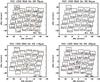 |
Fig. B.1 Maps of the OH emission from NGC 1333 IRAS 2A. The red and blue dashed lines indicate the rest wavelengths of the OH and CO transitions, respectively. |
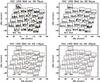 |
Fig. B.2 Maps of the OH emission from NGC 1333 IRAS 4A. The red and blue dashed lines indicate the rest wavelengths of the OH and CO transitions, respectively. Spaxels in gray were not included in the flux measurement. |
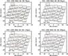 |
Fig. B.3 Maps of the OH emission from NGC 1333 IRAS 4B. The red and blue dashed lines indicate the rest wavelengths of the OH and CO transitions, respectively. Spaxels in gray were not included in the flux measurement. |
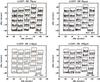 |
Fig. B.4 Maps of the OH emission from L 1527. The red and blue dashed lines indicate the rest wavelengths of the OH and CO transitions, respectively. |
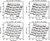 |
Fig. B.5 Maps of the OH emission from Ced 110 IRS 4. The red and blue dashed lines indicate the rest wavelengths of the OH and CO transitions, respectively. |
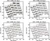 |
Fig. B.6 Maps of the OH emission from IRAS 15398. The red and blue dashed lines indicate the rest wavelengths of the OH and CO transitions, respectively. |
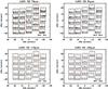 |
Fig. B.7 Maps of the OH emission from L 483. The red and blue dashed lines indicate the rest wavelengths of the OH and CO transitions, respectively. |
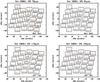 |
Fig. B.8 Maps of the OH emission from Ser SMM1. The red and blue dashed lines indicate the rest wavelengths of the OH and CO transitions, respectively. See also Goicoechea et al. (2012). |
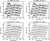 |
Fig. B.9 Maps of the OH emission from Ser SMM3. The red and blue dashed lines indicate the rest wavelengths of the OH and CO transitions, respectively. Spaxels in gray were not included in the flux measurement. |
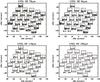 |
Fig. B.10 Maps of the OH emission from L 723. The red and blue dashed lines indicate the rest wavelengths of the OH and CO transitions, respectively. |
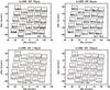 |
Fig. B.11 Maps of the OH emission from L 1489. The red and blue dashed lines indicate the rest wavelengths of the OH and CO transitions, respectively. |
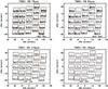 |
Fig. B.12 Maps of the OH emission from TMR 1. The red and blue dashed lines indicate the rest wavelengths of the OH and CO transitions, respectively. |
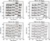 |
Fig. B.13 Maps of the OH emission from TMC 1A. The red and blue dashed lines indicate the rest wavelengths of the OH and CO transitions, respectively. |
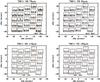 |
Fig. B.14 Maps of the OH emission from TMC 1. The red and blue dashed lines indicate the rest wavelengths of the OH and CO transitions, respectively. |
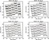 |
Fig. B.15 Maps of the OH emission from HH 46. The red and blue dashed lines indicate the rest wavelengths of the OH and CO transitions, respectively. |
 |
Fig. B.16 Maps of the OH emission from RNO 91. The red and blue dashed lines indicate the rest wavelengths of the OH and CO transitions, respectively. |
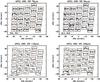 |
Fig. B.17 Maps of the OH emission from AFGL 490. The red and blue dashed lines indicate the rest wavelengths of the OH and CO transitions, respectively. |
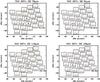 |
Fig. B.18 Maps of the OH emission from NGC 2071. The red and blue dashed lines indicate the rest wavelengths of the OH and CO transitions, respectively. |
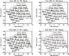 |
Fig. B.19 Maps of the OH emission from Vela IRS 17. The red and blue dashed lines indicate the rest wavelengths of the OH and CO transitions, respectively. |
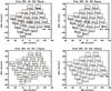 |
Fig. B.20 Maps of the OH emission from Vela IRS 19. The red and blue dashed lines indicate the rest wavelengths of the OH and CO transitions, respectively. |
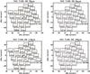 |
Fig. B.21 Maps of the OH emission from NGC 7129. The red and blue dashed lines indicate the rest wavelengths of the OH and CO transitions, respectively. |
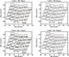 |
Fig. B.22 Maps of the OH emission from L 1641. The red and blue dashed lines indicate the rest wavelengths of the OH and CO transitions, respectively. |
Acknowledgments
We thank the referee for constructive comments that helped to improve the paper. The work on star formation at ETH Zurich is partially funded by the Swiss National Science Foundation (grant nr. 200020-113556). This program is made possible thanks to the Swiss HIFI guaranteed time program. WISH research in Leiden is supported by the Netherlands Research School for Astronomy (NOVA), by grant 614.001.008 from the Netherlands Organization for Scientific Research (NWO) and by EU-FP7 grant 238258 (LASSIE). HIFI has been designed and built by a consortium of institutes and university departments from across Europe, Canada and the United States under the leadership of SRON Netherlands Institute for Space Research, Groningen, The Netherlands and with major contributions from Germany, France and the US. Consortium members are: Canada: CSA, U.Waterloo; France: CESR, LAB, LERMA, IRAM; Germany: KOSMA, MPIfR, MPS; Ireland, NUI Maynooth; Italy: ASI, IFSI-INAF, Osservatorio Astrofisico di Arcetri – INAF; Netherlands: SRON, TUD; Poland: CAMK, CBK; Spain: Observatorio Astronómico Nacional (IGN), Centro de Astrobiología (CSIC-INTA). Sweden: Chalmers University of Technology – MC2, RSS & GARD; Onsala Space Observatory; Swedish National Space Board, Stockholm University – Stockholm Observatory; Switzerland: ETH Zurich, FHNW; USA: Caltech, JPL, NHSC.
References
- André, P., Ward-Thompson, D., & Barsony, M. 2000, Protostars and Planets IV, 59 [Google Scholar]
- Betz, A. L., &Boreiko, R. T. 1989, ApJ, 346, L101 [NASA ADS] [CrossRef] [PubMed] [Google Scholar]
- Bontemps, S.,André, P.,Terebey, S., &Cabrit, S. 1996, A&A, 311, 858 [NASA ADS] [Google Scholar]
- Brinch, C., &Hogerheijde, M. R. 2010, A&A, 523, A25 [NASA ADS] [CrossRef] [EDP Sciences] [Google Scholar]
- Butner, H. M., Evans, II, N. J.,Harvey, P. M., et al. 1990, ApJ, 364, 164 [NASA ADS] [CrossRef] [Google Scholar]
- Ceccarelli, C.,Caux, E.,White, G. J., et al. 1998, A&A, 331, 372 [NASA ADS] [Google Scholar]
- Crimier, N.,Ceccarelli, C.,Alonso-Albi, T., et al. 2010, A&A, 516, A102 [NASA ADS] [CrossRef] [EDP Sciences] [Google Scholar]
- Csengeri, T.,Menten, K. M.,Wyrowski, F., et al. 2012, A&A, 542, L8 [NASA ADS] [CrossRef] [EDP Sciences] [Google Scholar]
- de Geus, E. J., de Zeeuw, P. T., &Lub, J. 1989, A&A, 216, 44 [NASA ADS] [Google Scholar]
- de Graauw, T.,Helmich, F. P.,Phillips, T. G., et al. 2010, A&A, 518, L6 [NASA ADS] [CrossRef] [EDP Sciences] [Google Scholar]
- Dzib, S.,Loinard, L.,Mioduszewski, A. J., et al. 2010, ApJ, 718, 610 [NASA ADS] [CrossRef] [Google Scholar]
- Eiroa, C., Djupvik, A. A., & Casali, M. M. 2008, The Serpens Molecular Cloud, ed. B. Reipurth, 693 [Google Scholar]
- Elitzur, M. 1992, Astronomical masers (Dordrecht: Kluwer Academic Publishers), Astrophys. Space Sci. Lib., 170 [Google Scholar]
- Fich, M.,Johnstone, D., van Kempen, T. A., et al. 2010, A&A, 518, L86 [NASA ADS] [CrossRef] [EDP Sciences] [Google Scholar]
- Giannini, T.,Nisini, B., &Lorenzetti, D. 2001, ApJ, 555, 40 [NASA ADS] [CrossRef] [Google Scholar]
- Giannini, T.,Massi, F.,Podio, L., et al. 2005, A&A, 433, 941 [NASA ADS] [CrossRef] [EDP Sciences] [Google Scholar]
- Goicoechea, J. R., &Cernicharo, J. 2002, ApJ, 576, L77 [NASA ADS] [CrossRef] [Google Scholar]
- Goicoechea, J. R.,Rodríguez-Fernández, N. J., &Cernicharo, J. 2004, ApJ, 600, 214 [NASA ADS] [CrossRef] [Google Scholar]
- Goicoechea, J. R.,Cernicharo, J.,Lerate, M. R., et al. 2006, ApJ, 641, L49 [NASA ADS] [CrossRef] [Google Scholar]
- Goicoechea, J. R.,Joblin, C.,Contursi, A., et al. 2011, A&A, 530, L16 [NASA ADS] [CrossRef] [EDP Sciences] [Google Scholar]
- Goicoechea, J. R.,Cernicharo, J.,Karska, A., et al. 2012, A&A, 548, A77 [NASA ADS] [CrossRef] [EDP Sciences] [Google Scholar]
- Green, J. D., Evans II, N. J., Jørgensen, J. K., et al. 2013, ApJ, submitted [Google Scholar]
- Heathcote, S.,Morse, J. A.,Hartigan, P., et al. 1996, AJ, 112, 1141 [NASA ADS] [CrossRef] [Google Scholar]
- Herczeg, G. J.,Karska, A.,Bruderer, S., et al. 2012, A&A, 540, A84 [NASA ADS] [CrossRef] [EDP Sciences] [Google Scholar]
- Hirota, T.,Bushimata, T.,Choi, Y. K., et al. 2008, PASJ, 60, 37 [NASA ADS] [CrossRef] [Google Scholar]
- Hogerheijde, M. R., & van der Tak, F. F. S. 2000, A&A, 362, 697 [NASA ADS] [Google Scholar]
- Hollenbach, D., &McKee, C. F. 1980, ApJ, 241, L47 [NASA ADS] [CrossRef] [Google Scholar]
- Johnstone, D.,Fich, M.,Mitchell, G. F., &Moriarty-Schieven, G. 2001, ApJ, 559, 307 [NASA ADS] [CrossRef] [Google Scholar]
- Johnstone, D.,Fich, M.,McCoey, C., et al. 2010, A&A, 521, L41 [NASA ADS] [CrossRef] [EDP Sciences] [Google Scholar]
- Jørgensen, J. K.,Schöier, F. L., & van Dishoeck, E. F. 2002, A&A, 389, 908 [NASA ADS] [CrossRef] [EDP Sciences] [Google Scholar]
- Jørgensen, J. K.,Bourke, T. L.,Myers, P. C., et al. 2005, ApJ, 632, 973 [NASA ADS] [CrossRef] [Google Scholar]
- Karska, A., Herczeg, G. J., van Dishoeck, E. F., et al. 2013, A&A, in press, DOI: 10.1051/0004-6361/201220028 [Google Scholar]
- Kaufman, M. J., &Neufeld, D. A. 1996, ApJ, 456, 611 [NASA ADS] [CrossRef] [Google Scholar]
- Kenyon, S. J., Gómez, M., & Whitney, B. A. 2008, Low Mass Star Formation in the Taurus-Auriga Clouds, ed. B. Reipurth, 405 [Google Scholar]
- Knude, J., &Hog, E. 1998, A&A, 338, 897 [NASA ADS] [Google Scholar]
- Kristensen, L. E., van Dishoeck, E. F.,Bergin, E. A., et al. 2012, A&A, 542, A8 [NASA ADS] [CrossRef] [EDP Sciences] [Google Scholar]
- Larsson, B., Liseau, R., & Men’shchikov, A. B. 2002, A&A, 386, 1055 [NASA ADS] [CrossRef] [EDP Sciences] [Google Scholar]
- Lefloch, B.,Cabrit, S.,Codella, C., et al. 2010, A&A, 518, L113 [NASA ADS] [CrossRef] [EDP Sciences] [Google Scholar]
- Liseau, R.,Lorenzetti, D.,Nisini, B.,Spinoglio, L., &Moneti, A. 1992, A&A, 265, 577 [NASA ADS] [Google Scholar]
- Marseille, M. G., van der Tak, F. F. S.,Herpin, F., &Jacq, T. 2010, A&A, 522, A40 [NASA ADS] [CrossRef] [EDP Sciences] [Google Scholar]
- Massi, F.,Giannini, T.,Lorenzetti, D., et al. 1999, A&AS, 136, 471 [NASA ADS] [CrossRef] [EDP Sciences] [Google Scholar]
- Melnick, G. J.,Genzel, R., &Lugten, J. B. 1987, ApJ, 321, 530 [NASA ADS] [CrossRef] [Google Scholar]
- Mozurkewich, D.,Schwartz, P. R., &Smith, H. A. 1986, ApJ, 311, 371 [NASA ADS] [CrossRef] [Google Scholar]
- Neufeld, D. A., &Dalgarno, A. 1989a, ApJ, 340, 869 [NASA ADS] [CrossRef] [Google Scholar]
- Neufeld, D. A., &Dalgarno, A. 1989b, ApJ, 344, 251 [NASA ADS] [CrossRef] [Google Scholar]
- Nisini, B.,Giannini, T., &Lorenzetti, D. 2002, ApJ, 574, 246 [NASA ADS] [CrossRef] [Google Scholar]
- Nisini, B.,Benedettini, M.,Codella, C., et al. 2010, A&A, 518, L120 [NASA ADS] [CrossRef] [EDP Sciences] [Google Scholar]
- Offer, A. R., & van Dishoeck, E. F. 1992, MNRAS, 257, 377 [NASA ADS] [Google Scholar]
- Offer, A. R., van Hemert, M. C., & van Dishoeck, E. F. 1994, J. Chem. Phys., 100, 362 [NASA ADS] [CrossRef] [Google Scholar]
- Ossenkopf, V., &Henning, T. 1994, A&A, 291, 943 [NASA ADS] [Google Scholar]
- Ott, S. 2010, in Astronomical Data Analysis Software and Systems XIX, eds. Y. Mizumoto, K.-I. Morita, & M. Ohishi, ASP Conf. Ser., 434, 139 [Google Scholar]
- Pickett, H. M.,Poynter, I. R. L.,Cohen, E. A., et al. 1998, J. Quant. Spec. Radiat. Transf., 60, 883 [Google Scholar]
- Pilbratt, G. L.,Riedinger, J. R.,Passvogel, T., et al. 2010, A&A, 518, L1 [CrossRef] [EDP Sciences] [Google Scholar]
- Poglitsch, A.,Waelkens, C.,Geis, N., et al. 2010, A&A, 518, L2 [NASA ADS] [CrossRef] [EDP Sciences] [Google Scholar]
- Schöier, F. L., van der Tak, F. F. S., van Dishoeck, E. F., &Black, J. H. 2005, A&A, 432, 369 [NASA ADS] [CrossRef] [EDP Sciences] [Google Scholar]
- Schreyer, K.,Henning, T., van der Tak, F. F. S.,Boonman, A. M. S., & van Dishoeck, E. F. 2002, A&A, 394, 561 [NASA ADS] [CrossRef] [EDP Sciences] [Google Scholar]
- Schreyer, K.,Semenov, D.,Henning, T., &Forbrich, J. 2006, ApJ, 637, L129 [NASA ADS] [CrossRef] [Google Scholar]
- Shevchenko, V. S., &Yakubov, S. D. 1989, Sov. Astron., 33, 370 [NASA ADS] [Google Scholar]
- Snell, R. L.,Scoville, N. Z.,Sanders, D. B., &Erickson, N. R. 1984, ApJ, 284, 176 [NASA ADS] [CrossRef] [Google Scholar]
- Stanke, T.,McCaughrean, M. J., &Zinnecker, H. 2000, A&A, 355, 639 [NASA ADS] [Google Scholar]
- Takahashi, T.,Silk, J., &Hollenbach, D. J. 1983, ApJ, 275, 145 [NASA ADS] [CrossRef] [Google Scholar]
- van der Tak, F. F. S.,Black, J. H.,Schöier, F. L.,Jansen, D. J., & van Dishoeck, E. F. 2007, A&A, 468, 627 [NASA ADS] [CrossRef] [EDP Sciences] [Google Scholar]
- van Dishoeck, E. F.,Kristensen, L. E.,Benz, A. O., et al. 2011, PASP, 123, 138 [NASA ADS] [CrossRef] [Google Scholar]
- van Kempen, T. A.,Green, J. D.,Evans, N. J., et al. 2010a, A&A, 518, L128 [NASA ADS] [CrossRef] [EDP Sciences] [Google Scholar]
- van Kempen, T. A.,Kristensen, L. E.,Herczeg, G. J., et al. 2010b, A&A, 518, L121 [NASA ADS] [CrossRef] [EDP Sciences] [Google Scholar]
- van Kempen, T. A.,Longmore, S. N.,Johnstone, D.,Pillai, T., &Fuente, A. 2012, ApJ, 751, 137 [NASA ADS] [CrossRef] [Google Scholar]
- Vasta, M.,Codella, C.,Lorenzani, A., et al. 2012, A&A, 537, A98 [NASA ADS] [CrossRef] [EDP Sciences] [Google Scholar]
- Visser, R.,Kristensen, L. E.,Bruderer, S., et al. 2012, A&A, 537, A55 [NASA ADS] [CrossRef] [EDP Sciences] [Google Scholar]
- Wampfler, S. F.,Herczeg, G. J.,Bruderer, S., et al. 2010, A&A, 521, L36 [NASA ADS] [CrossRef] [EDP Sciences] [Google Scholar]
- Wampfler, S. F.,Bruderer, S.,Kristensen, L. E., et al. 2011, A&A, 531, L16 [NASA ADS] [CrossRef] [EDP Sciences] [Google Scholar]
- Whittet, D. C. B.,Prusti, T.,Franco, G. A. P., et al. 1997, A&A, 327, 1194 [NASA ADS] [Google Scholar]
- Wiesemeyer, H.,Güsten, R.,Heyminck, S., et al. 2012, A&A, 542, L7 [NASA ADS] [CrossRef] [EDP Sciences] [Google Scholar]
- Wilson, B. A.,Dame, T. M.,Masheder, M. R. W., &Thaddeus, P. 2005, A&A, 430, 523 [NASA ADS] [CrossRef] [EDP Sciences] [Google Scholar]
- Yıldız, U. A., van Dishoeck, E. F.,Kristensen, L. E., et al. 2010, A&A, 521, L40 [Google Scholar]
All Tables
Coordinates, distance, bolometric luminosity, and envelope masses of the low-mass class 0, class I, and intermediate-mass protostars in the sample.
Molecular data from the LAMDA database (Schöier et al. 2005) for the OH transitions detected with PACS.
OH fluxes used throughout the paper in units of 10-16 W m-2 with 1σ errors from the flux extraction.
Description whether the fluxes measured in the on-source spaxel and the surrounding three by three spaxels are consistent with the pure spillover factor (0.70 at 79 μm, 0.69 at 84 μm, 0.62 at 119 μm, and 0.49 at 163 μm).
Pearson’s correlation coefficients ρ, number of sources N, corresponding significance levels p, and number of standard deviations σ for the OH 84.6 μm line luminosity or flux and various envelope parameters.
H2O and [OI] fluxes of the intermediate-mass sources in units of 10-16 W m-2 measured on the full 5 by 5 array.
Resulting fluxes in units of 10-16 W m-2 in the spaxel with the strongest continuum (assumed to contain the central source position), corrected by the spillover factor (0.70 at 79 μm, 0.69 at 84 μm, 0.62 at 119 μm, and 0.49 at 163 μm).
All Figures
|
Fig. 1 OH transitions accessible with Herschel-PACS. Wavelengths are given in units of microns. Transitions that were observed for the entire source sample are shown in red. Transitions targeted only in the fraction of sources observed in range scan mode are depicted in blue if detected from at least one source and in gray if undetected. |
| In the text | |
|
Fig. 2 PACS line scan OH spectra of the low-mass class 0 young stellar objects in our sample. The x-axis is wavelengths in μm, the y-axis is continuum subtracted flux density in Jy (plus a constant offset). The red dashed lines indicate the rest frequencies of the OH transitions. The blue dotted line represents the rest frequency of CO(31–30), which is blended with OH at 84.42 μm. The sampling of range scans (Ser SMM1 and NGC 1333 IRAS 2A) is different from line scans. |
| In the text | |
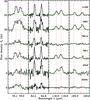 |
Fig. 3 Same as Fig. 2 but for the low-mass class I YSOs. |
| In the text | |
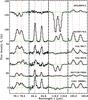 |
Fig. 4 Same as Fig. 2 but for the intermediate-mass protostars. |
| In the text | |
|
Fig. 5 Map of the OH 84 μm (red) and [OI] 63 μm emission (black) from NGC 2071, illustrating the similar spatial extent of the two transitions. The x-axis is velocity in km s-1, the y-axis continuum subtracted and normalized flux density. All spaxels were normalized with respect to the spaxel that contains the peak of the continuum emission at 63 μm. Note that the peak of the continuum emission at 84 μm falls onto the central spaxel, although the two observations were carried out consecutively. |
| In the text | |
|
Fig. 6 Map of the compact OH 84 μm emission from L 1489. The x-axis is wavelength in μm, the y-axis continuum subtracted and normalized flux density. All spaxels were normalized with respect to the central one. The red dashed lines indicate the rest frequencies of the OH transitions, the blue dashed line the CO(31–30). |
| In the text | |
|
Fig. 7 Map of spatially extended OH 119 μm absorption and emission from AFGL 490. The x-axis is wavelength in μm, the y-axis continuum subtracted and scaled flux density. The labels indicate the multiplicative scaling factors for each spaxel unless they are unity. |
| In the text | |
|
Fig. 8 Rotational diagram for the OH lines measured from Ser SMM1. Transitions belonging
to the |
| In the text | |
|
Fig. 9 OH luminosity of the 84 μm transition vs. bolometric luminosity of the source. Low-mass class 0 sources are shown as red diamonds, class I sources as blue triangles, and intermediate-mass protostars as green circles with 3σ error bars from the flux determination (does not include the calibration uncertainty). The dashed line is a linear fit to the data. |
| In the text | |
|
Fig. 10 OH 84 μm luminosity vs. envelope mass of the source. |
| In the text | |
|
Fig. 11 Bolometric luminosity vs. envelope mass of the sources. |
| In the text | |
|
Fig. 12 OH 84 μm luminosity vs. bolometric temperature of the sources. |
| In the text | |
|
Fig. 13 OH 84 μm luminosity vs. outflow force. |
| In the text | |
|
Fig. 14 OH 84 μm luminosity vs. luminosity to the 0.6 divided by the envelope mass of the sources (evolutionary tracer). |
| In the text | |
|
Fig. 15 Correlation of OH 84 μm luminosity with the 100 K radius of the spherical source models. |
| In the text | |
|
Fig. 16 Correlation of OH 84 μm luminosity with the H2 density at 1000 AU from the spherical source models. |
| In the text | |
|
Fig. 17 Correlation of OH 84 μm and [OI] 63 μm and 145 μm fluxes. |
| In the text | |
|
Fig. 18 Correlation of OH 84 μm and H2O 89.99 μm fluxes. |
| In the text | |
|
Fig. 19 OH 84 μm flux divided by H2O 89 μm flux vs. bolometric luminosity of the sources. Low-mass class I sources have a higher ratio than class 0 sources on average. |
| In the text | |
|
Fig. 20 OH 84 μm flux divided by H2O 89 μm flux vs. envelope mass of the sources. |
| In the text | |
|
Fig. 21 OH 84 μm flux divided by H2O 89 μm flux vs. bolometric temperature of the sources. |
| In the text | |
|
Fig. 22 OH 84 μm flux divided by H2O 89 μm flux vs. evolutionary tracer. |
| In the text | |
|
Fig. 23 Excitation temperature from slab models with Tgas = 200 K and Tdust = 100 K for the OH lines at 79, 84, 119, and 163 μm for OH column densities of 1014, 1016, and 1018 cm-2, and varying H2 density and dust column density. The dashed line indicates the critical density of the upper level of each transition, the dotted line marks where the dust becomes optically thick. |
| In the text | |
|
Fig. 24 Line flux ratios from slab models with Tgas = 200 K and Tdust = 100 K for the OH lines at 79, 84, 119, and 163 μm for OH column densities of 1014, 1016, and 1018 cm-2, and varying H2 density and dust column density. The shaded area marks the observed values. |
| In the text | |
|
Fig. 25 Comparison of the rotational diagram for the OH lines measured from Ser SMM1 (black diamonds) and a RADEX model with the source continuum included in the excitation (red plus signs) and a model without the continuum field of the source (blue plus signs). The model fluxes were scaled such that they match the observed 84.60 μm emission. The model including the continuum field reproduces the higher excited lines better than the one without. |
| In the text | |
|
Fig. 26 Correlation of OH 84 μm flux with the continuum fluxes measured from the PACS data at 63 μm and 84 μm. |
| In the text | |
|
Fig. B.1 Maps of the OH emission from NGC 1333 IRAS 2A. The red and blue dashed lines indicate the rest wavelengths of the OH and CO transitions, respectively. |
| In the text | |
|
Fig. B.2 Maps of the OH emission from NGC 1333 IRAS 4A. The red and blue dashed lines indicate the rest wavelengths of the OH and CO transitions, respectively. Spaxels in gray were not included in the flux measurement. |
| In the text | |
|
Fig. B.3 Maps of the OH emission from NGC 1333 IRAS 4B. The red and blue dashed lines indicate the rest wavelengths of the OH and CO transitions, respectively. Spaxels in gray were not included in the flux measurement. |
| In the text | |
|
Fig. B.4 Maps of the OH emission from L 1527. The red and blue dashed lines indicate the rest wavelengths of the OH and CO transitions, respectively. |
| In the text | |
|
Fig. B.5 Maps of the OH emission from Ced 110 IRS 4. The red and blue dashed lines indicate the rest wavelengths of the OH and CO transitions, respectively. |
| In the text | |
|
Fig. B.6 Maps of the OH emission from IRAS 15398. The red and blue dashed lines indicate the rest wavelengths of the OH and CO transitions, respectively. |
| In the text | |
|
Fig. B.7 Maps of the OH emission from L 483. The red and blue dashed lines indicate the rest wavelengths of the OH and CO transitions, respectively. |
| In the text | |
|
Fig. B.8 Maps of the OH emission from Ser SMM1. The red and blue dashed lines indicate the rest wavelengths of the OH and CO transitions, respectively. See also Goicoechea et al. (2012). |
| In the text | |
|
Fig. B.9 Maps of the OH emission from Ser SMM3. The red and blue dashed lines indicate the rest wavelengths of the OH and CO transitions, respectively. Spaxels in gray were not included in the flux measurement. |
| In the text | |
|
Fig. B.10 Maps of the OH emission from L 723. The red and blue dashed lines indicate the rest wavelengths of the OH and CO transitions, respectively. |
| In the text | |
|
Fig. B.11 Maps of the OH emission from L 1489. The red and blue dashed lines indicate the rest wavelengths of the OH and CO transitions, respectively. |
| In the text | |
|
Fig. B.12 Maps of the OH emission from TMR 1. The red and blue dashed lines indicate the rest wavelengths of the OH and CO transitions, respectively. |
| In the text | |
|
Fig. B.13 Maps of the OH emission from TMC 1A. The red and blue dashed lines indicate the rest wavelengths of the OH and CO transitions, respectively. |
| In the text | |
|
Fig. B.14 Maps of the OH emission from TMC 1. The red and blue dashed lines indicate the rest wavelengths of the OH and CO transitions, respectively. |
| In the text | |
|
Fig. B.15 Maps of the OH emission from HH 46. The red and blue dashed lines indicate the rest wavelengths of the OH and CO transitions, respectively. |
| In the text | |
|
Fig. B.16 Maps of the OH emission from RNO 91. The red and blue dashed lines indicate the rest wavelengths of the OH and CO transitions, respectively. |
| In the text | |
|
Fig. B.17 Maps of the OH emission from AFGL 490. The red and blue dashed lines indicate the rest wavelengths of the OH and CO transitions, respectively. |
| In the text | |
|
Fig. B.18 Maps of the OH emission from NGC 2071. The red and blue dashed lines indicate the rest wavelengths of the OH and CO transitions, respectively. |
| In the text | |
|
Fig. B.19 Maps of the OH emission from Vela IRS 17. The red and blue dashed lines indicate the rest wavelengths of the OH and CO transitions, respectively. |
| In the text | |
|
Fig. B.20 Maps of the OH emission from Vela IRS 19. The red and blue dashed lines indicate the rest wavelengths of the OH and CO transitions, respectively. |
| In the text | |
|
Fig. B.21 Maps of the OH emission from NGC 7129. The red and blue dashed lines indicate the rest wavelengths of the OH and CO transitions, respectively. |
| In the text | |
|
Fig. B.22 Maps of the OH emission from L 1641. The red and blue dashed lines indicate the rest wavelengths of the OH and CO transitions, respectively. |
| In the text | |
Current usage metrics show cumulative count of Article Views (full-text article views including HTML views, PDF and ePub downloads, according to the available data) and Abstracts Views on Vision4Press platform.
Data correspond to usage on the plateform after 2015. The current usage metrics is available 48-96 hours after online publication and is updated daily on week days.
Initial download of the metrics may take a while.