| Issue |
A&A
Volume 552, April 2013
|
|
|---|---|---|
| Article Number | A86 | |
| Number of page(s) | 12 | |
| Section | The Sun | |
| DOI | https://doi.org/10.1051/0004-6361/201219354 | |
| Published online | 03 April 2013 | |
Thermal and nonthermal hard X-ray source sizes in solar flares obtained from RHESSI observations
I. Observations and evaluation of methods
Leibniz-Institut für Astrophysik Potsdam (AIP),
An der Sternwarte 16,
14482
Potsdam,
Germany
e-mail:
This email address is being protected from spambots. You need JavaScript enabled to view it.
Received: 5 April 2012
Accepted: 26 February 2013
Abstract
Context. In solar flares, a large amount of thermal and nonthermal energy is released impulsively in the form of heated plasma and accelerated particles. These processes can be studied via hard X-ray (HXR) diagnostics. In addition to spectroscopic observations, a thorough understanding of the thermal and nonthermal particle populations requires the knowledge of the HXR source sizes.
Aims. We derive the geometric source parameters of both thermal coronal sources and the nonthermal HXR footpoints in solar flares. We compare and evaluate four different methods for obtaining source sizes, and then derive the most reliable source sizes, as well as the systematic uncertainties.
Methods. We obtained time series of HXR images for 24 flares from GOES class C3.4 to X17.2 using the RHESSI instrument. The four imaging techniques employed are CLEAN, Pixon, visibility forward fit, and MEM_NJIT. From this data set, we derived the geometric parameters of the thermal HXR sources and the nonthermal footpoints. Using the different imaging techniques allowed us to quantify systematic measurement uncertainties.
Results. We find that the different methods give consistent results on HXR source sizes. The correlations are very good for the thermal sources, and somewhat lower for the footpoints. The MEM_NJIT algorithm gives systematically smaller sizes than the other methods, possibly a result of over-resolution. Thermal source volumes are in the range of 2 × 1025−1.2 × 1028 cm3 (with a median relative uncertainty of 30%), and nonthermal footpoint areas in the range of 2 × 10¹⁶−6 × 1017 cm2 (median relative uncertainty: 40%). The thermal volumes of our sample are in the same range as those derived for microflares, which would imply that source size is not an important parameter for flare energetics.
Conclusions. Using different imaging algorithms for determining HXR source sizes offers the advantage that uncertainties can be better quantified thus making the derived parameters more reliable. Combined with geometric parameters that were derived as time series in a larger number of flares, this will allow the study of the scaling relations and the temporal evolution of thermal and nonthermal HXR sources.
Key words: Sun: flares / Sun: X-rays, gamma rays / acceleration of particles
© ESO, 2013
1. Introduction
In solar flares, a large amount of stored magnetic energy is impulsively released and converted to kinetic energy of nonthermal particles and bulk mass motions, and into thermal energy of hot plasmas, presumably within the framework of magnetic reconnection (cf. the standard CSHKP model of eruptive solar flares; Carmichael 1964; Sturrock 1966; Hirayama 1974; Kopp & Pneuman 1976). The nonthermal electrons, which carry a significant fraction of the energy released (e.g. Emslie et al. 2005), and the hot thermal plasma (T > 10 MK) are observed in the hard X-ray (HXR) and soft X-ray (SXR) regimes due to nonthermal and thermal bremsstrahlung as well as recombination radiation, respectively. The HXR observations (here, we refer to energies above 6 keV) are thus crucial for understanding the physics of energy release and particle acceleration in solar flares.
In recent years, the observational capabilities relevant to these questions have been increased substantially with the Ramaty High Energy Solar Spectroscopic Imager (RHESSI) spacecraft (Lin et al. 2002). Because of its high spectral resolution, RHESSI is the first instrument that provides a clear separation of the thermal from the nonthermal HXR emission. This allows the fitting of the photon spectra in order to obtain quantitative physical parameters of both thermal and nonthermal particle populations. However, spectral information is not sufficient for obtaining all relevant physical parameters. While the energy input of the nonthermal electrons above a certain low-energy cutoff can be readily obtained from the HXR spectrum (e.g. Holman et al. 2003), the computation of the thermal energy in the hot plasma requires knowledge of the plasma volume (e.g. Emslie et al. 2004; Veronig et al. 2005). Other important parameters include the thermal plasma density (e.g. Battaglia et al. 2009; Krucker et al. 2010) and the nonthermal electron flux density in the chromospheric footpoints, since high flux densities could lead to severe beam instabilities that may be inconsistent with the standard picture (see e.g. Melrose 1990; Benz 2002). This implies that for a full understanding of solar flares we require knowledge of both the thermal and nonthermal HXR source sizes. Because it is a spectroscopic imager, RHESSI is able to provide this information.
Imaging with RHESSI is not straightforward, since it does not rely on focusing optics which have not yet been implemented for the HXR range. Instead, the detected count rates from the incident X-rays are modulated by the imaging grids due to the rotation of the RHESSI spacecraft, and the amplitudes and phasing of the recorded time profiles encode the information on the HXR source positions, sizes, and shapes. There are various methods for recovering this information, called imaging algorithms (see Hurford et al. 2002; Aschwanden et al. 2004). Several of them have been used to measure source sizes. For example, several studies have used areas measured from images obtained with the CLEAN algorithm (e.g. Saint-Hilaire & Benz 2002, 2005; Veronig et al. 2005) in order to deduce thermal source volumes. Other studies have deduced thermal source sizes from modulation profiles (e.g. Schmahl & Hurford 2002; Saint-Hilaire & Benz 2002; Emslie et al. 2004), from Visibility Forward Fitting (e.g. Hannah et al. 2008) or from Pixon images (Veronig et al. 2005).
Most studies of source sizes conducted so far have had several limitations. Firstly, nearly all studies have focused on the peak times (either of the thermal or the nonthermal emission) of the flares, i.e. source sizes have been determined only for a single time interval. This approach ensures high count rates and thus reliable imaging thanks to good statistics, but it does not consider the temporal evolution of the sources. It is therefore not clear how far the sizes found are really representative of the whole flare duration. Secondly, many studies have used only a single method to determine source sizes, leaving open the question of whether different methods yield consistent results. This second issue has been dealt with extensively by Dennis & Pernak (2009), but only for nonthermal footpoint sources, and again only for HXR peaks. Thirdly, most studies are either case studies of one or a few events or, alternatively, of a larger number of flares with rather similar GOES importance. This means that systematic effects depending on the flare importance cannot be studied. Finally, because of the very different approaches and events considered in the different studies, a comparison of the results is difficult.
The aim of the present work is to accurately determine HXR source sizes in solar flares, in particular, thermal source volumes and nonthermal source areas. In order to proceed beyond previous works, we will (a) consider both thermal coronal sources and nonthermal footpoints; (b) use four different image reconstruction techniques to evaluate their characteristics and to quantify uncertainties; (c) determine the whole time evolution of the geometric parameters by using image time series; and (d) conduct these studies for 24 flares covering the range from mid-C-class to large X-class flares in order to study scaling relations.
This paper will focus on the observations and the comparison and evaluation of different methods for obtaining source sizes. In a following paper (Warmuth & Mann 2013, henceforth Paper II), we will use the results derived here to study scaling relationships and the temporal evolution of the geometric source parameters.
Observations, imaging methods, and the derivation of the source parameters are described in Sect. 2. The results given by the different methods are compared and discussed in Sect. 3, and the conclusions are given in Sect. 4.
2. Observations
2.1. Events
In order to study how the spatial characteristics of HXR sources change with flare importance, a larger sample of flares, from weak to very strong ones, needs to be analyzed. From the many events that RHESSI has observed since 2002, we have chosen 24 flares from GOES class C3.4 to X17.2 (7 C-class, 8 M-class, 8 X-class, and one greater than X10). We have not included smaller flares, since in those cases imaging would only be feasible close to the flare peaks. The flares were selected in order to cover some 2.5 decades of the GOES scale. They are listed in Table 1 in ascending order of GOES importance. Also shown are starting and maximum time of the GOES flare, and flare location.
A prerequisite for event selection was that the flares had to be well-observed by RHESSI and that they had to show – at least briefly during their evolution – a pair of nonthermal footpoints. This requirement will allow us to employ two independent methods for estimating coronal source volumes. The nonthermal count rate had to be high enough to obtain at least one image which allowed the unambiguous identification of the footpoint pair for integration times of ≤60 s. This resulted in nonthermal images with ≥3000 counts (actually for most images, several 10 000 counts).
This selection criterion imposes a minimum geometric size for the flares selected for this study, as it excludes flares with very closely spaced footpoints, as well as flares where one footpoint is very weak or limb-occulted. We have compared the GOES characteristics of the selected flares to the whole ensemble of GOES flares of solar cycle 23. This showed that the selected events tend to have shorter SXR rise times than the mean rise times of the total sample. This is particularly pronounced in the weaker flares: while the selected X-ray flares show similar rise times to the average, the selected C-class flares have rise times that are two to three times shorter. In other words, the selected flares, in particular the weaker ones, are more impulsive than the average flare sample, and there are no particularly gradual events or LDEs. The majority of our flares showed eruptive activity – 88% were associated with coronal mass ejections (CMEs), and 75% with metric type II radio bursts, which are signatures of coronal shock waves.
Many of the flares in our sample have been used for comparison with the results of a shock-drift acceleration model (Mann et al. 2009; Warmuth et al. 2009), and for the study of nonthermal energetics in the framework of magnetic reconnection (Mann & Warmuth 2011). All events have HXR data coverage from the onset of the impulsive phase until after its end, with the exception of the X17.2 flare of 2003 Oct. 28, where RHESSI missed the peak of the impulsive phase, but which was nevertheless included as an example for an outstandingly large flare.
List of the 24 flares analyzed.
2.2. Imaging
2.2.1. Energy ranges and temporal resolution
For imaging the thermal coronal sources, we used the energy range of 6−12 keV. This regime is nearly always dominated by thermal free-free emission and additionally contains a Fe-Ni line complex. We have verified spectroscopically that we are indeed imaging the thermal plasma. For the nonthermal sources, we used energy ranges that were individually selected for each event in order to contain only nonthermal emission. This was verified by spectroscopy. Typical energy ranges were 25−50 keV for smaller flares, 50−100 keV for larger flares, and 100−300 keV in one case (2003 Oct. 28). In each event, the same energy range was used for all four image reconstruction methods.
The time binning was chosen in order to adequately resolve the temporal evolution of the sources (this includes covering the rise phase of the thermal component in at least three time steps and separating the major nonthermal HXR peaks) and to provide sufficient counts (≥1000) for imaging. The count rate of course changes with the flares’ evolution, so the time bins represent a compromise. For the thermal component, we used either 20 or 60 s (in 10 and 14 events, respectively). The nonthermal time bins ranged from 16 to 60 s. Again, in each event the image reconstruction methods used the same binning.
2.2.2. Image reconstruction methods and grid selection
Following Dennis & Pernak (2009), we used four different image reconstruction methods – the main imaging algorithms employed with RHESSI. The first method is the much-used CLEAN algorithm (see Hurford et al. 2002). Generally, imaging with RHESSI is sensitive to the subcollimators which are used, since each subcollimator produces a modulation of the HXR count rate only if there are source structures with dimensions at or below the resolution of that grid. Otherwise, this subcollimator will only add noise. In particular, source dimensions are sensitive to the finest subcollimator that is being used, and to the relative weighting of the different grids.
As there is currently no automated way to specify the optimum choice of grids and weighting, we have adopted the following strategy. Grid selection was achieved by checking whether the back projection images from each individual subcollimator showed only noise or signatures of a source. This was done for the peak times of both the thermal and nonthermal emission (with energy ranges as defined above) for all flares. We then verified our grid selection by producing CLEAN images with the two different weighting schemes that are available, natural weighting, where each grid is weighted equally, and uniform weighting, which gives more weight to the finer grids and thus reduces side lobes. If the final image was too noisy or the sources were broken up, we dropped the finest subcollimator used, which always solved this problem.
For most of the events we identified grid 3 as the minimum that should be used for the thermal source (for two events: grid 4, and for one: grid 1)1. For the nonthermal component, natural weighting allowed us to use grid 1 as the finest subcollimator in all events but one (2003 Oct. 28, for which grid 2 had to be used). With uniform weighting, this was only possible in four events, while for 18 events grid 2 had to be chosen (in two events: grid 3). Grids 8 and 9 were adopted as the coarsest subcollimators. We then produced image series with the time, energy, and grid parameters as determined above, for all the time ranges with detectable thermal and nonthermal HXR emission. For this paper, we have chosen to use the geometric parameters derived from CLEAN with natural weighting (see discussion in Sect. 2.3), which will henceforth be referred to as CLN.
The second imaging algorithm used is Pixon (henceforth PIX; see Metcalf et al. 1996), which is widely believed to provide the most accurate photometry (Alexander et al. 1997) and the simplest model for the image that is consistent with the data (Puetter 1995). We generally used the same grid selection as for the CLN images.
The third imaging method used is the visibility forward fit (VFF) algorithm (Hurford et al. 2005), a visibility-based method that iteratively determines the best-fit parameters of a simple assumed source geometry. Source models include circular, elliptical, and curved elliptical Gaussians. Despite this limitation, which rules out complex sources, the VFF method has several advantages. The geometric source parameters do not have to be extracted from the images, but are obtained directly, with statistical errors. Furthermore, grid selection is not critical with the VFF method, since subcollimators dominated by noise have little influence on the fit.
We started our application of the VFF method by fitting all thermal sources with elliptical Gaussians. Where this failed − because of non-converging fits or unacceptably large errors − we tried using alternative source models. We found that in most events the thermal sources were well-fitted by elliptical Gaussians. In two flares, a part of the sources had to be fitted by curved Gaussians (i.e. loops), and in three other events all thermal sources were better reproduced by the curved Gaussians. A single event was fitted by circular Gaussians. The footpoint sources were always fitted by two circular Gaussians (note that Dennis & Pernak 2009 have used a modified VFF method that allows for two elliptical Gaussians).
As the last imaging algorithm, we used another visibility-based method, namely MEM_NJIT (henceforth MNJ; see Schmahl et al. 2007), a maximum-entropy method. While MNJ has a tendency to break up larger sources, it potentially allows “super-resolution” up to two to three times better than the instrument’s PSF (e.g. Cornwell & Evans 1985). For the MNJ images, we generally used the same grid parameters as for the CLEAN images with uniform weighting.
The number of images produced with each of the four methods was about 600 images for the thermal and 120 images for the nonthermal components, adding up to a total of 2882 HXR images.
2.3. Definition and measurement of geometric source parameters
Since there is no stereoscopic HXR imaging available, we have to derive source volumes from 2D maps. Commonly, a geometric scaling is applied to obtain volume V from source area A via V = A3/2, with the area usually being defined by the 50% contour level of the source. Another option is to adopt the FWHM of a 2D Gaussian fitted to the source as the linear dimensions. We settled for the latter method to be consistent with the VFF method, using the IDL routine GAUSS2DFIT. The major and minor FWHM sizes of the fitted source ellipse, wa and wb, are obtained from the sigmas of the Gaussian via  (1)We used this approach for the CLN, PIX, and MNJ images. For the CLN sources, there is a complication: we have to deconvolve for the CLEAN beam by quadratically subtracting the FWHM of the beam from the measured FWHM of the source to obtain the true dimensions (cf. Saint-Hilaire & Benz 2002). While this is easily done for a large number of images, the method tends to overcorrect in small sources, i.e. the measured FWHMs are smaller than the CLEAN beam, and thus either wb becomes negative, or both wa and wb become negative. This was the case in a substantial fraction of the footpoint sources. An alternative method was developed by (Dennis & Pernak 2009): this approach uses the CLEAN components (i.e. point sources) and thus avoids the complications of the CLEAN beam deconvolution. We have therefore adopted this method for deriving our footpoint source sizes. Applying the same method to the thermal sources, we subsequently found a somewhat lower correlation with the sizes given by the other image reconstruction techniques. Thus, we have chosen to retain the deconvolution method for the thermal sources. We have opted to use the naturally weighted CLEAN images in this study, since the derived paramaters correlate slightly better with the other image reconstruction methods than those obtained with uniform weighting. However, doing the whole analysis using uniform weighting instead, or using either the deconvolution or the CLEAN component method, has a very minor effect on the results presented in this paper and Paper II.
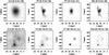 |
Fig. 1 RHESSI images obtained with different reconstruction methods. Shown are images from the peak of the impulsive phase of the M8.2 flare on 2002 Apr. 10. The top row shows the thermal source imaged at 6−12 keV. In the bottom row, the nonthermal footpoints are visible in 50−100 keV images. From left to right, the imaging methods used are CLEAN with natural weighting (CLN), Pixon (PIX), visibility forward fit (VFF), and MEM_NJIT (MNJ). The white ellipses depict the FWHM of 2D Gaussian sources fitted to the images (for CLN, the Gaussians are derived from the CLEAN components; for VFF, they are the forward-fitted sources). The number of the finest grid used for image synthesis is shown on top of each plot. |
When the VFF forward-fitting method is used, the major and minor axes are given directly by the fitting algorithm. One limitation with VFF was that we used circular sources for the footpoints, i.e. wa = wb.
From the size of the Gaussian sources, we can then compute the source areas by 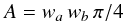 (2)for the thermal source (Ath) and the nonthermal footpoints (Anth,1, Anth,2). The total footpoint area is the sum of the areas of the two footpoints, Anth,tot = Anth,1 + Anth,2.
The volume of the thermal source can now be obtained with two different approaches. We can measure the thermal source size (direct method) and derive the thermal volume Vdir from the area Ath via 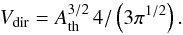 (3)The numerical factor in this equation is obtained from the conversion of area to volume for a spherical source. It is usually omitted since the uncertainties of volume estimations are generally significantly larger.
Alternatively, we can measure the nonthermal footpoint areas and their separation, and assume that the thermal plasma is contained in a semicircular loop or torus connecting them (indirect method). According to this approach, we get the volume Vind by 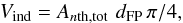 (4)
(4)
where dFP is the distance between the centroids of the two fitted footpoint sources (corrected for foreshortening). Note that for the computation of both Vdir and Vind, a filling factor of unity was assumed.
2.4. Source detection
In total, the number of thermal sources measured (over all events and time steps) was 593, 587, 432, and 561 for CLN, PIX, VFF, and MNJ, respectively. The lower number of VFF sources is because the fits either did not converge or yielded very large errors on the fit parameters in a significant fraction of time intervals (fits with relative errors ≥1 were discarded). This may have been caused because the actual source structures were significantly more complex than the assumed simple geometries (cf. Dennis & Pernak 2009). The number of MNJ sources is slightly reduced owing to the break up of some larger sources, which were then excluded from further analysis.
The corresponding number of measured footpoints was 232, 231, 186, and 241 for the four imaging methods. The lower number for VFF is due to the same issues as for the thermal sources. In particular, sources with lower count rates often yielded large fit uncertainties.
2.5. General morphology
All flares showed a thermal coronal source and – at least in one time interval – a pair of nonthermal footpoints, as required by the event selection criteria. While the average time span during which the thermal sources were observed was 19 min, the footpoints were visible only for 6 min on average. While geometrically small flares tended to be consistent with simple source morphologies – a compact coronal source lying above and between two compact footpoints – some larger flares showed more structure, such as complex and fragmented coronal sources.
As an example for a medium-sized event, Fig. 1 shows the RHESSI images reconstructed with different imaging methods from the peak of the impulsive phase of the M8.2 flare on 2002 Apr. 10. It is evident that all imaging methods have adequately reproduced the general morphology – a thermal coronal source and two nonthermal footpoints. Closer inspection reveals some notable differences, however. For example, MNJ produces some fracturing of the thermal source. Whether this is real super-resolution or an artifact is not clear. As for the higher energies, CLN, PIX, and MNJ give some indication of smaller and weaker nonthermal sources north of the footpoints. VFF, naturally, does not show these sources. Thus it is evident that the different imaging methods will also yield somewhat differing source sizes. We will study this issue in the following section.
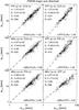 |
Fig. 2 Comparison of the major axes wa,th (FWHM) of the thermal sources for all flares and time intervals. Measurements obtained from the four different image reconstruction algorithms (LN, PIX, VFF, MNJ) are plotted against each other. Only cotemporal measurements are included. Also shown are power-law fits using the OLS bisector method (dashed lines), the slope and intercept of the obtained power-law, α and b, the linear correlation coefficient, C, and the number of value pairs, N. The dotted lines denote x = y. At the bottom of the plots, the mean ratio (⟨ .../... ⟩) of wa,th obtained from the two methods that are compared is shown. |
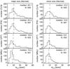 |
Fig. 4 Distribution of the thermal source sizes obtained with the four imaging methods. Plotted are histograms of the major axes wa,th (left) and minor axes wb,th (right). Dashed lines indicate the median of the distributions. Also given is the number of measurements N. |
3. Discussion
3.1. Comparison and distribution of source sizes
3.1.1. Thermal coronal sources
We can now begin to evaluate the different imaging techniques by comparing the derived source sizes. In Fig. 2, the major axes of the thermal components wa,th, as given by the different techniques, are plotted against each other. Only cotemporal measurements are included.
The power-law fits shown in the plots were derived with the ordinary least-squares (OLS) bisector method (Isobe et al. 1990), which is based on two OLS regression fits on the data, or in this case, on the logs of the data – log x on log y and log y on log x. The bisector of these two lines is then obtained as log y = b + αlog x, and the corresponding power-law is y = 10bxα, with α as the slope and b as the intercept. The advantage of this method is that it treats both variables symmetrically − and so to be preferred for establishing functional relationships when the distinction between dependent and independent variables is not clear, and when the scatter is fairly large. In addition to the power-law parameters α and b (including standard deviation), the plots show the linear correlation coefficient C, and the number of value pairs N. At the bottom of the plots, the mean of the axes’ ratios is indicated.
The different imaging methods show an excellent correlation for wa,th, with correlation coefficients C ≥ 0.85 for all cases. The correlation is best between CLN and PIX (C = 0.93). The mean ratios show that while CLN, PIX, and VFF give consistent results, the MNJ values for the major axes are systematically lower by some 15% on average. Figure 3 shows the same comparison for the minor axes of the thermal components, wb,th. They are equally well-correlated, with coefficients C ≥ 0.75, and again the sizes given by MNJ are generally smaller than for the other methods, by up to 17%.
The corresponding distributions of wa,th and wb,th as given by the four imaging methods, together with the medians of the distributions, are shown in Fig. 4. Generally the different distributions are consistent: wa,th starts at minimum values around 5′′, peaks between 15′′ and 20′′, and extends up to 70′′–80′′. In the case of MNJ, the distribution peaks at lower values and extends only up to 60′′. The distributions of the minor axis wb,th peak around 10′′ and reach a maximum of about 30′′.
We thus conclude that the four imaging techniques all yield consistent results on the thermal source sizes. Besides a random scatter, the only systematic trend is that MNJ gives somewhat smaller (≈15%) source sizes.
The distributions of the thermal source sizes can be compared to the results of Hannah et al. (2008) derived with the VFF method for a large sample of microflares. Their distributions of wa,th and wb,th have similar shapes to ours, but extend to larger sizes. Their median of wa,th is larger than ours (31 6 vs. ≈20′′), while the median of wb,th (105) is consistent with ours. The microflare sources are thus more elongated than ours (median aspect ratio wb,th/wa,th of 0.34 vs. ≈0.5). This may be because we mainly used elliptical Gaussians, while Hannah et al. (2008) exclusively used curved Gaussians (i.e. loops), which may yield larger axis ratios. While it is somewhat surprising that an ensemble of microflares would have comparable or even larger average source sizes than a sample containing much stronger flares, Hannah et al. (2008) found no evidence for a correlation between source size and flare magnitude, so this result is not totally unexpected. They have suggested that this finding could be due to a prevalence of a typical loop scale size associated with active regions, which would be consistent with our results. We will nevertheless investigate the issue of a possible correlation between thermal source size and flare importance for our sample in Paper II.
3.1.2. Nonthermal footpoint sources
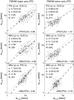 |
Fig. 5 As Fig. 2, but showing both the major (left column) and minor axes (right column) of the nonthermal footpoints wa,nth and wb,nth. Since the VFF method employs circular sources, only the correlations between values obtained from the three other algorithms are shown. |
The major and minor axes of the nonthermal footpoint sources wa,nth and wb,nth, as given by the different imaging methods, are compared in Fig. 5 (left and right column, respectively). Note that we have not included the VFF algorithm in this comparison since VFF assumes circular footpoints (wa,nth = wb,nth), which would result in systematically smaller major and larger minor axes compared to the other methods. The major axes are reasonably well correlated (C ≥ 0.59). Again the MNJ values are smaller than the ones given by the other methods. With 20−30% on average, this size difference is more pronounced than for the thermal sources. The correlations for the minor axes are lower than for the major ones (C ≤ 0.53). The PIX sources are wider than the CLN sources, while the MNJ sources are consistent with CLN. Also note that the deviations from a linear relationship are more pronounced for the footpoint axes compared to the thermal sources.
In order to allow a sensible comparison with the nonthermal source sizes as given by VFF, the correlations between the footpoint areas Anth,FP derived from the four methods are shown in Fig. 6. This comparison shows that the nonthermal VFF source areas are indeed reasonably well correlated with the ones given by the other methods (C involving VFF is 0.5−0.66). The only systematic trend apparent is once again the smaller (by 20−30%) MNJ area. Note that the total nonthermal source areas (Anth,tot, not shown here) given by the different methods correlate slightly better (with a mean C of 0.67) than the individual footpoint areas (mean C: 0.61).
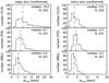 |
Fig. 7 As Fig. 4, but showing histograms of the major and minor axes of the nonthermal footpoint sources wa,nth and wb,nth (here, the VFF method is excluded). |
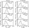 |
Fig. 8 As Fig. 4, but showing histograms of the nonthermal footpoint areas Anth,FP (left column), and the footpoint separation dFP (right column). |
The distributions of wa,nth and wb,nth (see Fig. 7) as given by the different methods (again excluding VFF) show slightly larger differences than in the case of the thermal sources. For CLN and PIX, wa,nth has a median near between 8′′ and 10′′ and extends up to ≈30′′, while the MNJ distribution has a lower median at 62. For wb,nth, both CLN and MNJ peak around 3′′, while PIX peaks near 4′′2. All three distributions extend to 8′′–10′′. These characteristics are also evident in the distributions of the footpoint areas Anth,FP shown in the left column of Fig. 8. While the median is .4 × 1017 cm2 for CLN, 1.5 × 1017 cm2 for PIX, and 1.3 × 1017 cm2 for VFF, it is significantly lower with 8.5 × 1016 cm2 for MNJ.
While the nonthermal source sizes as derived from the four imaging methods thus show both a larger scatter and more pronounced systematic differences than the thermal sources do, they are still consistent. In particular, CLN, PIX, and VFF are in good agreement, while MNJ yields sources smaller by about 40% in terms of area. This behaviour is similar but more pronounced than in the case of the thermal sources.
These results can now be compared to the results of Dennis & Pernak (2009), who have derived nonthermal footpoint sizes for the HXR peaks of 18 flares using PIXON, MEM_NJIT, and modified versions of CLEAN and VFF. They found good correlations for the major axes as given by the four different methods, with correlation coefficients in the same range as ours. Poorer correlations (C ≤ 0.51) were obtained for the minor axes, which is also similar to our experience. With their four methods, Dennis & Pernak (2009) found mean values of 52−75 for the major footpoint axis, and 23−34 for the minor axis. While our results are within the same range, our linear source sizes are larger by about 20% on average.
This small but systematic difference could be caused by multiple factors. Dennis & Pernak (2009) have employed methods specifically tailored for small compact sources, while we have worked with the standard imaging procedures. They have derived source parameters only for the main HXR peak in each event and could thus individually optimize imaging parameters such as integration time. In contrast, we have derived time series covering a larger fraction of the flare and were thus forced to make compromises. However, an even more important aspect is grid selection. While Dennis & Pernak (2009) have always included the finest grid for imaging, we have individually chosen the grids according to the scheme described in Sect. 2.2 – this has resulted in using grid 2 as the finest subcollimator for MNJ in most events. We have additionally produced all nonthermal MNJ images using grid 1. The footpoint sizes wa,nth and wb,nth became consistent with the results of Dennis & Pernak (2009), but the fraction of sources that had to be discarded because of fragmentation was much higher. The correlations between the various methods also declined significantly when grid 1 was used in all cases, especially for wb,nth.
Our results are thus consistent with those of Dennis & Pernak (2009), who have taken these poor correlations as a sign that this dimension is actually not well measured by RHESSI. By individually selecting the grids for each event and method, we have achieved a slightly better correlation between the different methods and have minimized the occurrence of source fracturing. This could imply that using the finest grid may not always be the best way to determine nonthermal source sizes. However, even with this individual selection the correlations for the minor footpoint axes do not improve dramatically, which suggests that this quantity is indeed not well measured by RHESSI.
Finally, we have also compared the footpoint separations dFP. Here, we found excellent agreement between all methods, with correlations C ≥ 0.98, α ≈ 1, and mean differences between the various methods of 1−3%. The corresponding distributions are shown in the right column of Fig. 8. They are all consistent, peak around 25−30 Mm, and extend up to 85 Mm. This consistency was to be expected since determining the source location with RHESSI depends only on the knowledge of the phases of the different grid pairs, and not on the relative sensitivities of the different subcollimators, which are much less accurately known.
3.2. Measurement uncertainties, averages, and selection of optimum methods
After having verified that the four imaging methods generally give consistent results on source sizes, we now want to determine which method should be chosen to obtain the most reliable measurements. Prior to that, we have to evaluate whether the differences found between the different methods are actually significant. This requires a quantification of measurement uncertainties. The imaging algorithm VFF is currently the only one that provides the statistical ± 1σ uncertainties of the source parameters. In the top row of Fig. 9, histograms of the relative uncertainties (defined as σVFF divided by the fitted value of the source parameter) are shown for the axes of the thermal and nonthermal sources given by VFF (note that wa,nth = wb,nth). The medians of these relative uncertainties are 6% for wa,th, 9% for wb,th, and 13% for wa,nth.
We now compute the mean values of the source sizes by averaging over all four algorithms in all events and time intervals. The corresponding standard deviation is a measure of how consistent all methods are, or in other words, of the systematic uncertainties. The resulting relative uncertainties (σ normalized by the mean value) are shown in the middle row of Fig. 9. The medians of these deviations are 14% for wa,th, 17% for wb,th, and 27% for both wa,nth and wb,nth (for the latter two quantities, VFF was excluded). Thus these standard deviations are about twice as large as the statistical uncertainties given by VFF, which shows that the differences given by the four algorithms are indeed significant – though not large – for a large fraction of the measured sources. Most of the values given by the four methods are within ±2σVFF from the mean value: the medians of these differences − given in terms of σVFF – range from 0.9 to 1.9 for the thermal sources, and from 0.8 to 2.3 for the nonthermal ones. The differences from the mean vary according to imaging method and source type. For instance, with medians of 1.9 and 1.3 σVFF for wa,th and wb,th, MNJ shows the largest deviations from the mean of the thermal source sizes. This implies that at least for a non-negligible fraction of thermal sources, MNJ might not be the most appropriate imaging algorithm.
We have thus chosen to select the best imaging algorithms for each event individually. For each event, time series of the relevant parameters as given by the four methods were generated. As an example, Fig. 10 shows these time series for the M8.2 flare on 2002 Apr. 10 that was already depicted in Fig. 1. These plots demonstrate, for example, that while all methods show good agreement for the footpoint sizes in the first time interval, the VFF method (shown in blue) gives exceedingly large values for the second nonthermal time interval (see middle and bottom row in Fig. 10). The VFF method was thus discarded for the nonthermal sources in this event. Accordingly, in each event, if one algorithm showed stark disagreement with the other three methods, it was discarded. The mean values and standard deviations were then computed from the three remaining algorithms.
For the thermal sources, PIX, VFF, and MNJ were discarded in 2, 6, and 8 events, respectively. The high number of events where MNJ was rejected is a result of the problems with over-resolution and source breakup mentioned above and discussed in Sect. 4. In contrast, CLN was retained in all events. In the nonthermal case, VFF was discarded in two events, and PIX and MNJ in one event each. The low overall number of rejected nonthermal sources results from the fact that despite the larger scatter between the footpoint sizes it was usually not possible to identify one single deviant method. Instead, the four methods tended to give more equally separated values.
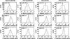 |
Fig. 9 Distributions of the relative uncertainty – defined as the standard deviation σ divided by the mean of the measured values – for the major and minor axes of the thermal and nonthermal sources (from left to right: wa,th, wb,th, wa,nth, and wb,nth). Top row: relative statistical uncertainties given by the VFF forward fitting method. Middle row: relative systematic uncertainties derived from the four imaging methods. Bottom row: relative systematic uncertainties derived from those imaging methods that have been individually selected for each event. |
The relative deviation of the source sizes resulting from using only the individually selected methods are shown in the bottom row of Fig. 9. For the thermal sources, the medians of the relative deviations have been reduced significantly by rejecting MNJ in a third of the events, while in the nonthermal case, the distributions are very similar because in only a few cases methods could be rejected. The relative uncertainties obtained from the different methods are now closer to the statistical uncertainties as given by VFF, but are still about twice as large.
We thus adopt the values given by our selected methods as the most probable source sizes. All further analysis – also in Paper II – will be based on these parameters. At the same time, the corresponding standard deviations provide an estimate of the total uncertainties (while the standard deviations actually reflect the systematic uncertainties, we have shown above that they are significantly larger than the statistical uncertainties). Generally, the uncertainties are at the 10% level for the linear thermal source sizes, corresponding to 30% uncertainty for the thermal volumes Vdir. The nonthermal linear source sizes show higher uncertainties of about 25%. The corresponding median relative uncertainty is 40% for the footpoint areas, and 30% for the indirectly determined thermal volumes Vind.
Finally, we stress that the individual selection of methods has no strong influence on any of the derived results, either in this paper or in Paper II. We have also conducted the whole analysis without rejecting methods in individual events, and apart from slightly reduced correlation coefficients, all results remained virtually unchanged. Incidentally, this is also true when different combinations of imaging methods involving other CLEAN methods (see Sect. 2.2) were used. We thus conclude that our results are derived from a reasonably robust basis.
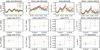 |
Fig. 10 Temporal evolution of the geometric HXR source parameters as determined by the four different image reconstruction methods, shown for the example of the M8.2 flare of 2002 Apr. 10. The top row shows the major and minor axes wa,th and wa,th, area Ath, and volume Vdir of the thermal source. The middle and bottom rows show the axes wa,nth and wb,nth, and areas Anth of the two footpoint sources, as well as the thermal volume Vind and the footpoint separation dFP. |
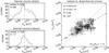 |
Fig. 11 Left: distribution of the thermal source volumes obtained with the direct and indirect methods, Vdir (top) and Vind (bottom), as derived from the optimum imaging algorithms individually selected for each event. Dashed lines indicate the median of the distributions. Also given is the number of measurements N. Right: comparison of Vdir and Vind. Only cotemporal measurements are included. Error bars show the standard deviation from the different imaging methods. Also shown is a power-law fit (dashed line, with slope α), the rank correlation coefficient R, and the number of value pairs N. The dotted line denotes x = y. At the bottom of the plot, the mean ratio ⟨ Vdir/Vind ⟩ is shown. |
3.3. Thermal source volumes
We can now finally obtain the definite values of the thermal source volumes as given by the direct and the indirect method. Histograms of Vdir and Vind are shown in Fig. 11. Both distributions are broadly comparable, with comparable medians of 5.5 × 1026 cm3 for Vdir and 5.7 × 1026 cm3 for Vind. However, the distribution for Vdir is broader, ranging over almost three magnitudes from a minimum of 2 × 1025 cm3 up to 1.2 × 1028 cm3, while Vind ranges only over less than two magnitudes from 7 × 1025 cm3 to 3 × 1027 cm3.
At the right side of Fig. 11, a scatter plot shows the correlation of Vdir and Vind (only cotemporal measurements are included). It is evident that generally a larger Vdir is associated with larger Vind, although there is significant scatter. In contrast to the previous plots, the power-law here has been obtained with the bivariate correlated errors and instrincic scatter (BCES) bisector estimator (Akritas & Bershady 1996). This method is similar to OLS bisector in the sense that the fit is given by the bisector of two linear regression fits. In contrast to OLS, BCES accounts for measurement errors in x and y, and is therefore preferred for cases where there are significant and well-defined uncertainties. With a power-law index of α = 0.63 (for comparison, OLS bisector gives α = 0.67), the relationship is distinctly nonlinear. In this case, Spearman’s rank correlation coefficient R is a more appropriate measure of the correlation than the linear correlation coefficient C used throughout this paper. This gives a moderate but significant correlation with R = 0.58. Note the data point with Vdir and Vind below 1026 cm3: this is the C6.2 flare 2002 Oct. 05. In this event, the two footpoints are so close together that they can barely be separated. It thus reflects the lower size limit that is imposed by our event selection criteria (see Sect. 2.1).
Note that we found a closer agreement between Vdir and Vind than did the study of Saint-Hilaire & Benz (2005), whose Vind was always much larger than Vdir. A comparison with our values shows that while Saint-Hilaire & Benz (2005) obtained comparable direct volumes, their indirect volumes were systematically larger than ours by up to an order of magnitude. This is probably because they did not use the finer grids for obtaining the nonthermal images. What is consistent between the two studies is that the power-law index of the correlation between Vdir and Vind is significantly below unity. This means that the product of the footpoint areas and their separation grows at a lower rate than the corresponding volume obtained directly from the thermal source size.
As already noted in Sect. 3.1, it is interesting that our distributions of volumes are consistent with the distribution derived for microflares by Hannah et al. (2008) – their median volume of 1027 cm3 is even larger than ours. This would imply that the geometric size of a flare is not a major determining factor for its energetics, which is at odds with studies using EUV and SXR data which did find a scaling between flare length scale and energetics (e.g. Ofman et al. 1996; Aschwanden & Parnell 2002; Aschwanden & Aschwanden 2008). We will return to consider this issue in more detail in Paper II.
Having the choice between Vdir and Vind, which method should be preferred to obtain the most realistic source volumes? The direct method has the advantages that it uses the actual thermal emission and relies on fewer assumptions – basically only the scaling from area to volume. In contrast, Vind has to assume a semicircular loop between the nonthermal footpoints. This assumption could easily be wrong, since hot thermal plasma can also be present in loops in which electrons are not – or no longer – accelerated, and which therefore are not associated with nonthermal footpoint emission. In this case, Vind would underestimate the actual volume. The fact that for larger volumes, Vind is indeed smaller than Vdir (see Fig. 11) is an indication that this is actually the case, at least in larger flares. Conversely, the many cases where Vind > Vdir could be because the footpoint sizes – particularly the minor axes – are not well measured (see Sect. 3.1.2) and may thus not be completely resolved. Such a notion is supported by the observation of sub-arcsecond structures in white-light flare footpoints (e.g. Hudson et al. 2006; Jess et al. 2008).
Another limitation of the indirect method is statistics: the nonthermal sources always have significantly fewer counts than the thermal ones. Imaging is thus possible only during the comparatively short time range of impulsive HXR emission, and even then the temporal resolution and total time range is severely limited by statistics. In many events it is thus not possible to really study the evolution of Vind. In particular, in many cases Vind is not available at the time of maximum thermal emission, where knowledge of the volume is most desirable, since this is probably close to the time of maximum thermal energy.
The indirect method has one advantage, though: at times, the thermal sources can be quite fragmented (we have tried to minimize this fracturing by careful grid selection, see Sect. 2.2.2) and complex, which makes a quantitative determination of the source size somewhat ambiguous. The footpoints, however, tend to stay compact and can thus be measured more accuartely. Whether Vind really reflects the thermal volume in such a case, or whether it severely underestimates the volume (see discussion above), is of course debatable. In any case, determining both Vdir and Vind in an event provides two independent measures of source volume that can be checked against each other. Any severe disagreement found could be a useful indication of a potential problem, since generally the disagreement between Vdir and Vind is not too large (see Fig. 11).
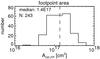 |
Fig. 12 As Fig. 4, but showing the distribution of the nonthermal footpoint areas Anth,FP as derived from the optimum imaging algorithms individually selected for each event. |
3.4. Nonthermal source areas
Figure 12 shows the distribution that is finally derived for the nonthermal footpoint areas Anth,FP according the scheme introduced in Sect. 3.2. The distribution extends from 2 × 1016 cm2 to 6 × 1017 cm2 and has a median of 1.4 × 1017 cm2. These results are consistent with other studies which found footpoint sizes comparable with the resolution of the finest grids (e.g. Fletcher et al. 2007; Schmahl et al. 2007; Kontar et al. 2008; Dennis & Pernak 2009). Our footpoints tend to be larger than those derived by Dennis & Pernak (2009) by a factor of 1.5 in terms of area. As already discussed in Sect. 3.1, this is probably due to differing imaging methods and, most importantly, grid selection schemes. We conclude that imaging with RHESSI does approach its limits when it comes to the sizes of the compact nonthermal footpoints – particularly when the minor axis is concerned – but the derived areas are probably accurate to a factor of less than two.
One caveat with the nonthermal source sizes is that they could potentially be affected by albedo (e.g. Kontar & Jeffrey 2010): backscattered photons will increase the measured source sizes in the energy range between 10 and 100 keV. Most of our footpoint sizes and areas are upper limits where the measurements of the minor axes are upper limits. However, these upper limits are not likely to have been significantly increased by the albedo since Battaglia et al. (2011) have shown that albedo increases the FWHM of a footpoint by less than 30%. The presence of extended albedo sources can in principle be inferred in the presence of compact footpoint sources from the relative intensities of the modulation amplitudes given by the finer and coarser subcollimators (Schmahl & Hurford 2002). However, this does not unambigously show that the extended sources are due to albedo (instead of being a direct coronal signature). Note that the Pixon algorithm is generally regarded as the best method to image extended sources in the presence of compact ones. Hence, it should be most affected when there are strong albedo sources. However, since we found no strong disagreement between the source dimensions given by the different methods, we conclude that there is no significant albedo contribution to the source sizes as measured here.
4. Conclusions
We have derived both thermal and nonthermal HXR source sizes from RHESSI observations of 24 flares, ranging from GOES class C to large X-class flares. The focus in this paper was on evaluating and comparing different methods of obtaining source sizes, to identify those that give the most reliable measures, and to quantify measurement uncertainties. As imaging algorithms, we considered CLEAN, Pixon, VFF, and MEM_NJIT.
We evaluated two different methods of deriving source dimensions from CLEAN images – deconvolving for the CLEAN beam (e.g. Saint-Hilaire & Benz 2002), and using the CLEAN components (Dennis & Pernak 2009). The methods give comparable results, and we have finally adopted the deconvolution technique for the thermal sources, and the component method for the footpoints, since this choice maximizes both the agreement with the other methods and the number of sources that could be measured.
Overall, the CLEAN and Pixon methods have proven to be the most stable techniques, while VFF had problems in some particular cases, probably because of complex sources. The comparison of the different methods has shown that the sizes of the thermal coronal sources as given by the different methods agree quite well, with the exception of MEM_NJIT, which gives systematically smaller thermal source sizes. In addition, MEM_NJIT has a tendency to break up larger sources, even when care is given to grid selection. From that, we conclude that MEM_NJIT should be used with care when it comes to thermal coronal sources, and that it is not well-suited for larger sources.
For the nonthermal footpoints, the source sizes given by the different methods are generally also in agreement, although the correlation is less pronounced than for the thermal sources. Again, MEM_NJIT gives the smallest source sizes.
Thus, MEM_NJIT is the single algorithm that gives systematically different results compared to the other image reconstruction techniques – it yields smaller source sizes for both thermal and nonthermal sources. This is probably because of super-resolution – an inherent property of any MEM-based algorithm. Super-resolution means going beyond the resolving power of the instrument by effectively providing an extrapolation of the data in the spatial frequency plane towards larger spatial frequencies. This has been pointed out by Cornwell & Evans (1985) and Schmahl et al. (2007). However, this particular property is currently not well understood (cf. Dennis & Pernak 2009), thus it is not clear whether this merely represents over-resolution (which gives artificially small sources) or whether it provides additional information of the source.
Using four different methods allowed us to obtain the most probable values for source sizes, and also to assess the possible uncertainties. By comparing the time series of the geometric parameters, we rejected inappropriate imaging methods for each individual event (and source type). The mean of the values given by the remaining selected methods was then adopted as the definite value for the parameter, while the standard deviation reflects the systematic uncertainties. Since these dominate the statistical uncertainties, we have adopted the standard deviation as an estimate of the total uncertainties.
We have assumed a filling factor of unity in this paper, therefore all thermal volumes and nonthermal footpoint areas derived here are actually upper limits. We have found thermal source volumes ranging from 2 × 1025 cm3 to 1.2 × 1028 cm3 when using the sizes of the thermal source (“direct method”), and from 7 × 1025 cm3 to 3 × 1027 cm3 when computing the thermal volume from the areas and the separation of the footpoints (“indirect method"). The median of the relative uncertainties of the thermal volumes is on the order of 30%.
One issue that has complicated comparisons of thermal source sizes in the past was that some studies used the direct method, while others employed the indirect method, and both methods seemed to give very different results (see Saint-Hilaire & Benz 2005). In contrast to this, we have shown that both methods give comparable results, provided that particular care is given to the issue of RHESSI grid selection. Generally, the direct method should be preferred, since it relies on fewer assumptions, has better statistics, and the thermal source can be followed over a longer time range. However, the indirect method provides an independent check and can be employed to identify potential problems with the thermal volumes.
It is very interesting to note that the distributions of our thermal volumes are basically comparable to the one derived by Hannah et al. (2008) for a large sample of RHESSI microflares. The fact that our C to X class flares have similar sizes to microflares would imply that the geometric size or source volume is not an important parameter for determining flare energetics. While this is consistent with the lack of a correlation between source size and microflare magnitude found by Hannah et al. (2008), it contrasts with other studies using SXR and EUV data (e.g. Ofman et al. 1996; Aschwanden & Aschwanden 2008). We will study this issue further in Paper II.
We found nonthermal footpoint areas in the range of 2 × 10¹⁶−6 × 1017 cm2, with a median relative error of 40% (the median error is 32% when MNJ – which gives systematically smaller footpoints – is not included at all). These areas are larger by factors around 1.5 than those derived by Dennis & Pernak (2009), which could be explained by different image reconstruction techniques and grid selection strategies: while the latter study used methods specifically tailored for compact footpoints and always employed grid 1 as the finest subcollimator, we used the standard imaging techniques and have individually selected
the grids for each event. This disagreement and the relatively large measurement uncertainties imply that RHESSI imaging reaches its limits when it comes to very compact footpoints, which is in agreement with the conclusion of Dennis & Pernak (2009) that the minor axis of the footpoints is not well measured by RHESSI. This notion is also consistent with observations of white-light flares that show footpoints with structures well below RHESSI’s resolution limit of 2′′ (e.g. Hudson et al. 2006; Jess et al. 2008).
While this paper has been technical in focusing on the systematic comparison and evaluation of methods for obtaining source sizes, this was a necessary step before we could study the scaling relations and the evolution of thermal volumes and nonthermal footpoint areas with any confidence. This will be done in the companion Paper II. In another upcoming paper, we will combine the geometric parameters with RHESSI HXR spectroscopy in order to study the energy partition in solar flares.
Note that grid 2 cannot be used for the thermal sources since the low-energy threshold of the corresponding detector is 20 keV.
For comparison, the median of the VFF-derived values for wa,nth = wb,nth is 56.
Acknowledgments
The work of A.W. was supported by DLR under grant No. 50 QL 0001. The authors are grateful to the RHESSI Team (PI: R. P. Lin) for the free access to the data and the development of the software.
References
- Akritas, M. G., & Bershady, M. A. 1996, ApJ, 470, 706 [NASA ADS] [CrossRef] [Google Scholar]
- Alexander, D., Metcalf, T., & Hudson, H. S. 1997, in Magnetic Reconnection in the Solar Atmosphere, eds. R. D. Bentley, & J. T. Mariska (San Francisco: ASP), ASP Conf. Ser., 111, 253 [Google Scholar]
- Aschwanden, M. J., & Aschwanden, P. D. 2008, ApJ, 674, 544 [NASA ADS] [CrossRef] [Google Scholar]
- Aschwanden, M. J., & Parnell, C. E. 2002, ApJ, 572, 1048 [NASA ADS] [CrossRef] [Google Scholar]
- Aschwanden, M. J., Metcalf, T. R., Krucker, S., et al. 2004, Sol. Phys., 219, 149 [NASA ADS] [CrossRef] [Google Scholar]
- Battaglia, M., Fletcher, L., & Benz, A. O. 2009, A&A, 498, 891 [NASA ADS] [CrossRef] [EDP Sciences] [Google Scholar]
- Battaglia, M., Kontar, E. P., & Hannah, I. G. 2011, A&A, 526, A3 [NASA ADS] [CrossRef] [EDP Sciences] [Google Scholar]
- Benz, A. 2002, Plasma Astrophysics, 2nd edn. (Springer) [Google Scholar]
- Carmichael, H. 1964, NASA SP, 50, 451 [Google Scholar]
- Cornwell, T. J., & Evans, K. F. 1985, A&A, 143, 77 [NASA ADS] [Google Scholar]
- Dennis, B. R., & Pernak, R. L. 2009, ApJ, 698, 2131 [NASA ADS] [CrossRef] [Google Scholar]
- Emslie, A. G., Kucharek, H., Dennis, B. R., et al. 2004, J. Geophys. Res., 109, 10104 [NASA ADS] [CrossRef] [Google Scholar]
- Emslie, A. G., Dennis, B. R., Holman, G. D., & Hudson, H. S. 2005, J. Geophys. Res., 110, 11103 [NASA ADS] [CrossRef] [Google Scholar]
- Fletcher, L., Hannah, I. G., Hudson, H. S., & Metcalf, T. R. 2007, ApJ, 656, 1187 [NASA ADS] [CrossRef] [Google Scholar]
- Hannah, I. G., Christe, S., Krucker, S., et al. 2008, ApJ, 677, 704 [NASA ADS] [CrossRef] [Google Scholar]
- Hirayama, T. 1974, Sol. Phys., 34, 323 [NASA ADS] [CrossRef] [Google Scholar]
- Holman, G. D., Sui, L., Schwartz, R. A., & Emslie, A. G. 2003, ApJ, 595, L97 [NASA ADS] [CrossRef] [Google Scholar]
- Hudson, H. S., Wolfson, C. J., & Metcalf, T. R. 2006, Sol. Phys., 234, 79 [NASA ADS] [CrossRef] [Google Scholar]
- Hurford, G. J., Schmahl, E. J., Schwartz, R. A., et al. 2002, Sol. Phys., 210, 61 [NASA ADS] [CrossRef] [Google Scholar]
- Hurford, G. J., Schmahl, E. J., & Schwartz, R. A. 2005, AGU Abstr. Spring, A12 [Google Scholar]
- Isobe, T., Feigelson, E. D., Akritas, M. G., & Babu, G. J. 1990, ApJ, 364, 104 [NASA ADS] [CrossRef] [EDP Sciences] [Google Scholar]
- Jess, D., Mathioudakis, M., Crockett, P. J., & Keenan, F. P. 2008, ApJ, 688, L119 [NASA ADS] [CrossRef] [Google Scholar]
- Kontar, E. P., & Jeffrey, N. L. S. 2010, A&A, 513, L2 [NASA ADS] [CrossRef] [EDP Sciences] [Google Scholar]
- Kontar, E. P., Hannah, I. G., & MacKinnon, A. L. 2008, A&A, 489, L57 [NASA ADS] [CrossRef] [EDP Sciences] [Google Scholar]
- Kopp, R. A., & Pneuman, G. W. 1976, Sol. Phys., 50, 85 [NASA ADS] [CrossRef] [Google Scholar]
- Krucker, S., Hudson, H. S., Glesener, L., et al. 2010, ApJ, 714, 1108 [NASA ADS] [CrossRef] [Google Scholar]
- Lin, R. P., Dennis, B. R., Hurford, G. J., et al. 2002, Sol. Phys., 210, 3 [Google Scholar]
- Mann, G., & Warmuth, A. 2011, A&A, 528, A104 [NASA ADS] [CrossRef] [EDP Sciences] [Google Scholar]
- Mann, G., Warmuth, A., & Aurass, H. 2009, A&A, 494, 669 [NASA ADS] [CrossRef] [EDP Sciences] [Google Scholar]
- Melrose, D. B. 1990, Sol. Phys., 130, 3 [NASA ADS] [CrossRef] [Google Scholar]
- Metcalf, T. R., Hudson, H. S., Kosugi, T., Puetter, R. C., & Pina, R. K. 1996, ApJ, 466, 585 [NASA ADS] [CrossRef] [Google Scholar]
- Ofman, L., Davila, J. M., & Shimizu, T. 1996, ApJ, 459, L39 [NASA ADS] [CrossRef] [Google Scholar]
- Puetter, R. C. 1995, Int. J. Image Sys., & Tech., 6, 314 [Google Scholar]
- Saint-Hilaire, P., & Benz, A. O. 2002, Sol. Phys., 210, 287 [NASA ADS] [CrossRef] [Google Scholar]
- Saint-Hilaire, P., & Benz, A. O. 2005, A&A, 435, 743 [NASA ADS] [CrossRef] [EDP Sciences] [Google Scholar]
- Schmahl, E. J., & Hurford, G. J. 2002, Sol. Phys., 210, 273 [NASA ADS] [CrossRef] [Google Scholar]
- Schmahl, E. J., Pernak, R. L., Hurford, G. J., Lee, J., & Bong, S. 2007, Sol. Phys., 240, 241 [NASA ADS] [CrossRef] [Google Scholar]
- Sturrock, P. A. 1966, Nature, 211, 695 [NASA ADS] [CrossRef] [Google Scholar]
- Veronig, A. M., Brown, J. C., Dennis, B. R., et al. 2005, ApJ, 621, 482 [Google Scholar]
- Warmuth, A., & Mann, G. 2013, A&A, 552, A87 [NASA ADS] [CrossRef] [EDP Sciences] [Google Scholar]
- Warmuth, A., Mann, G., & Aurass, H. 2009, A&A, 494, 677 [NASA ADS] [CrossRef] [EDP Sciences] [Google Scholar]
All Tables
All Figures
|
Fig. 1 RHESSI images obtained with different reconstruction methods. Shown are images from the peak of the impulsive phase of the M8.2 flare on 2002 Apr. 10. The top row shows the thermal source imaged at 6−12 keV. In the bottom row, the nonthermal footpoints are visible in 50−100 keV images. From left to right, the imaging methods used are CLEAN with natural weighting (CLN), Pixon (PIX), visibility forward fit (VFF), and MEM_NJIT (MNJ). The white ellipses depict the FWHM of 2D Gaussian sources fitted to the images (for CLN, the Gaussians are derived from the CLEAN components; for VFF, they are the forward-fitted sources). The number of the finest grid used for image synthesis is shown on top of each plot. |
| In the text | |
|
Fig. 2 Comparison of the major axes wa,th (FWHM) of the thermal sources for all flares and time intervals. Measurements obtained from the four different image reconstruction algorithms (LN, PIX, VFF, MNJ) are plotted against each other. Only cotemporal measurements are included. Also shown are power-law fits using the OLS bisector method (dashed lines), the slope and intercept of the obtained power-law, α and b, the linear correlation coefficient, C, and the number of value pairs, N. The dotted lines denote x = y. At the bottom of the plots, the mean ratio (⟨ .../... ⟩) of wa,th obtained from the two methods that are compared is shown. |
| In the text | |
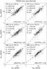 |
Fig. 3 As Fig. 2, but showing the minor axes wb,th of the thermal sources. |
| In the text | |
|
Fig. 4 Distribution of the thermal source sizes obtained with the four imaging methods. Plotted are histograms of the major axes wa,th (left) and minor axes wb,th (right). Dashed lines indicate the median of the distributions. Also given is the number of measurements N. |
| In the text | |
|
Fig. 5 As Fig. 2, but showing both the major (left column) and minor axes (right column) of the nonthermal footpoints wa,nth and wb,nth. Since the VFF method employs circular sources, only the correlations between values obtained from the three other algorithms are shown. |
| In the text | |
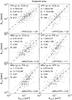 |
Fig. 6 As Fig. 2, but comparing areas of the nonthermal footpoint sources, Anth,FP. |
| In the text | |
|
Fig. 7 As Fig. 4, but showing histograms of the major and minor axes of the nonthermal footpoint sources wa,nth and wb,nth (here, the VFF method is excluded). |
| In the text | |
|
Fig. 8 As Fig. 4, but showing histograms of the nonthermal footpoint areas Anth,FP (left column), and the footpoint separation dFP (right column). |
| In the text | |
|
Fig. 9 Distributions of the relative uncertainty – defined as the standard deviation σ divided by the mean of the measured values – for the major and minor axes of the thermal and nonthermal sources (from left to right: wa,th, wb,th, wa,nth, and wb,nth). Top row: relative statistical uncertainties given by the VFF forward fitting method. Middle row: relative systematic uncertainties derived from the four imaging methods. Bottom row: relative systematic uncertainties derived from those imaging methods that have been individually selected for each event. |
| In the text | |
|
Fig. 10 Temporal evolution of the geometric HXR source parameters as determined by the four different image reconstruction methods, shown for the example of the M8.2 flare of 2002 Apr. 10. The top row shows the major and minor axes wa,th and wa,th, area Ath, and volume Vdir of the thermal source. The middle and bottom rows show the axes wa,nth and wb,nth, and areas Anth of the two footpoint sources, as well as the thermal volume Vind and the footpoint separation dFP. |
| In the text | |
|
Fig. 11 Left: distribution of the thermal source volumes obtained with the direct and indirect methods, Vdir (top) and Vind (bottom), as derived from the optimum imaging algorithms individually selected for each event. Dashed lines indicate the median of the distributions. Also given is the number of measurements N. Right: comparison of Vdir and Vind. Only cotemporal measurements are included. Error bars show the standard deviation from the different imaging methods. Also shown is a power-law fit (dashed line, with slope α), the rank correlation coefficient R, and the number of value pairs N. The dotted line denotes x = y. At the bottom of the plot, the mean ratio ⟨ Vdir/Vind ⟩ is shown. |
| In the text | |
|
Fig. 12 As Fig. 4, but showing the distribution of the nonthermal footpoint areas Anth,FP as derived from the optimum imaging algorithms individually selected for each event. |
| In the text | |
Current usage metrics show cumulative count of Article Views (full-text article views including HTML views, PDF and ePub downloads, according to the available data) and Abstracts Views on Vision4Press platform.
Data correspond to usage on the plateform after 2015. The current usage metrics is available 48-96 hours after online publication and is updated daily on week days.
Initial download of the metrics may take a while.