| Issue |
A&A
Volume 551, March 2013
|
|
|---|---|---|
| Article Number | A107 | |
| Number of page(s) | 26 | |
| Section | Stellar atmospheres | |
| DOI | https://doi.org/10.1051/0004-6361/201220921 | |
| Published online | 04 March 2013 | |
X-shooter spectroscopy of young stellar objects
II. Impact of chromospheric emission on accretion rate estimates⋆,⋆⋆
1
European Southern Observatory, Karl Schwarzschild Str. 2, 85748
Garching, Germany
e-mail:
This email address is being protected from spambots. You need JavaScript enabled to view it.
2
INAF − Osservatorio Astrofisico di Arcetri,
Largo E. Fermi 5, 50125
Firenze,
Italy
3
Department of Planetary Science, Lunar and Planetary Lab,
University of Arizona, 1629, E. University Blvd, Tucson
AZ
85719,
USA
4
INAF − Osservatorio Astronomico di Capodimonte,
via Moiariello 16, 80131
Napoli,
Italy
5
School of Cosmic Physics, Dublin Institute for Advanced
Studies, 31 Fitzwilliam
Place, Dublin 2,
Ireland
6
INAF − Osservatorio Astronomico di Palermo,
Piazza del Parlamento 1,
90134
Palermo,
Italy
7
INAF − Osservatorio Astronomico di Brera,
via Bianchi 46, 23807
Merate ( LC), Italy
8
INAF − Osservatorio Astronomico di Trieste,
via Tiepolo 11, 34143
Trieste,
Italy
9
INAF − Osservatorio Astronomico di Roma,
via di Frascati 33,
00040
Monte Porzio Catone ( RM), Italy
Received:
14
December
2012
Accepted:
10
January
2013
Abstract
Context. The lack of knowledge of photospheric parameters and the level of chromospheric activity in young low-mass pre-main sequence stars introduces uncertainties when measuring mass accretion rates in accreting (Class II) young stellar objects. A detailed investigation of the effect of chromospheric emission on the estimates of mass accretion rate in young low-mass stars is still missing. This can be undertaken using samples of young diskless (Class III) K and M-type stars.
Aims. Our goal is to measure the chromospheric activity of Class III pre main sequence stars to determine its effect on the estimates of the accretion luminosity (Lacc) and mass accretion rate (Ṁacc) in young stellar objects with disks.
Methods. Using VLT/X-shooter spectra, we analyzed a sample of 24 nonaccreting young stellar objects of spectral type between K5 and M9.5. We identified the main emission lines normally used as tracers of accretion in Class II objects, and we determined their fluxes in order to estimate the contribution of the chromospheric activity to the line luminosity.
Results. We have used the relationships between line luminosity and accretion luminosity derived in the literature for Class II objects to evaluate the impact of chromospheric activity on the accretion rate measurements. We find that the typical chromospheric activity would bias the derived accretion luminosity by Lacc,noise< 10-3 L⊙, with a strong dependence on the Teff of the objects. The noise on Ṁacc depends on stellar mass and age, and the typical values of log(Ṁacc,noise) range between ~−9.2 to −11.6 M⊙/yr.
Conclusions. Values of Lacc ≲10-3 L⊙ obtained in accreting low-mass pre main sequence stars through line luminosity should be treated with caution because the line emission may be dominated by the contribution of chromospheric activity.
Key words: stars: pre-main sequence / stars: low-mass / stars: activity
Based on observations collected in the programs 084.C-0269, 085.C-0238, 086.C-0173, 087.C-0244, 089.C-0143 at the European Organization for Astronomical Research in the Southern Hemisphere (Chile).
Tables 6, 7, and Appendices are available in electronic form at http://www.aanda.org
© ESO, 2013
1. Introduction
Circumstellar disks are formed as a natural consequence of angular momentum conservation during the gravitational collapse of cloud cores (e.g. Shu et al. 1987). In the early phases of star formation, the disk allows for the dissipation of angular momentum channeling the accretion of material from the infalling envelope onto the central young stellar object (YSO). At later stages, when the envelope is dissipated, planetary systems form in the disk, while the star-disk interaction continues through the inner disk and the stellar magnetosphere. This phenomenon constrains the final stellar mass build-up (e.g. Hartmann et al. 1998), and its typical timescales are connected with the timescales on which disks dissipate and planet formation occurs (e.g. Hernández et al. 2007; Fedele et al. 2010; Williams & Cieza 2011).
Accretion can be observed using typical signatures in the spectra of YSOs, such as the continuum excess in the blue part of the visible spectrum (e.g. Gullbring et al. 1998) and the prominent optical and infrared emission lines (e.g. Muzerolle et al. 1998a,b; Natta et al. 2004; Herczeg & Hillenbrand 2008; Rigliaco et al. 2012). The measurements used to determine the bolometric accretion luminosity (Lacc) are either direct or indirect. Direct measurements are obtained by measuring the emission in excess of the photospheric one in the Balmer and Paschen continua and adopting a model to correct for the emission at the wavelengths not covered by the observations, which originates mostly below the U-band threshold (e.g. Valenti et al. 1993; Gullbring et al. 1998; Calvet & Gullbring 1998; Herczeg & Hillenbrand 2008; Rigliaco et al. 2012) or by line profile modeling (e.g. Muzerolle et al. 1998a,b). Indirect measurements are obtained using empirical correlations between emission line luminosity (Lline) and Lacc (e.g. Muzerolle et al. 1998a,b; Natta et al. 2004, 2006; Mohanty et al. 2005; Rigliaco et al. 2011).
Measurements of mass accretion rate (Ṁacc) are subjected to many uncertainties, because this quantity depends on Lacc and on the mass-to-radius (M∗/R∗) ratio. This ratio is normally determined from the position of the object on the HR diagram and a set of evolutionary models. Uncertainties on spectral type (SpT) of the objects affect the determination of effective temperature (Teff), while those on the extinction (AV) and the distance mainly affect the estimate of stellar luminosity (L∗). It is not trivial to determine those parameters in accreting stars because of accretion shocks on the stellar surface producing veiling in the photospheric lines (e.g. Calvet & Gullbring 1998) and modifying the photometric colors (e.g. Da Rio et al. 2010). Moreover, the derivation of Lline, from which Lacc is determined, is affected by another stellar property, namely the chromospheric activity of the YSOs (Houdebine et al. 1996; Franchini et al. 1998). Chromospheric line emission is usually smaller than the accretion-powered emission, but it can become important when accretion decreases at later evolutionary stages (Ingleby et al. 2011) and in lower mass stars, where accretion rates are lower (Rigliaco et al. 2012). Therefore, this is an important source of uncertainty that has not been investigated in detail so far.
Part of the INAF consortium’s guaranteed time observations (GTO) of X-shooter, a broad-band, medium-resolution, high-sensitivity spectrograph mounted on the ESO/VLT, has been allocated for star formation studies, in particular to investigate accretion, outflows, and chromospheric emission in low-mass Class II young stellar and substellar objects (Alcalá et al. 2011). The targets observed during the GTO were chosen in nearby (d < 500 pc) star forming regions with low extinction and with many very low-mass (VLM) YSO (M∗ < 0.2 M⊙). Generally, those YSOs for which measurements in many photometric bands were available, both in the IR (e.g. Hernández et al. 2007; Merín et al. 2008) and in the visible part of the spectrum (e.g. Merín et al. 2008; Rigliaco et al. 2011), were selected. To derive Lacc of a given Class II YSO, a Class III template of the same SpT as the Class II is needed. Therefore, during this GTO survey 24 Class III targets in the range K5−M9.5 were observed, providing the first broad-band grid of template spectra for low-mass stars and brown dwarfs (BDs). Since these spectra have a very wide wavelength range (~350−2500 nm) covering part of the UV spectrum (UVB), the whole visible (VIS), and the near infrared (NIR), this sample allows us to determine the stellar parameters of the targets, derive the chromospheric emission line fluxes and luminosities, hence determine the implications of chromospheric emission on the indirect accretion estimates in Class II objects.
The paper is structured as follows. In Sect. 2 we discuss the sample selection, the observation strategy, and the data reduction procedure. In Sect. 3 we describe how SpTs of our targets have been determined, while in Sect. 4 we derive their main stellar parameters. In Sect. 5 we identify the main lines present in the spectra and derive their intensities. In Sect. 6 we discuss the implications of the line luminosity found for studies of Ṁacc in Class II YSOs. Finally, in Sect. 7 we summarize our conclusions.
2. Sample, observations, and data reduction
Among the objects observed in the GTO survey, we selected only those that have been classified as Class III objects using Spitzer photometric data. The sample comprises Class III YSOs in the σ Orionis, Lupus III, and TW Hya associations. In the end, the number of targets is 24: 13 objects are members of the TW Hya association, 6 of the Lupus III cloud, and 5 of the σ Orionis region. Their SpTs range between K5 and M9.5 (see Sect. 3). Three BDs, namely Par-Lup3-1, TWA26, and TWA29, are included in our sample, with SpT M6.5, M9, and M9.5, respectively. Data available from the literature for these objects are reported in Table 1. Six YSOs in our sample are components of three known wide visual binary systems. In all cases we were able to resolve them, given that their separations are always larger than 6′′.
All the observations were made in the slit-nodding mode, in order to achieve a good sky subtraction. Different exposure times and slit dimensions were used for different targets to have enough signal-to-noise ratio (S/N) and to avoid saturation. The readout mode used in all the observations was “100, 1 × 1, hg”, while the resolution of our spectra is R = 9100, 5100, and 3300 in the UVB arm for slits 0.5′′, 1.0′′, and 1.6′′, respectively; R = 17 400, 8800, and 5400 in the VIS arm for slits 0.4′′, 0.9′′, and 1.5′′, respectively; R = 11 300, 5600, and 3500 in the NIR arm for slits 0.4′′, 0.9′′, and 1.5′′, respectively. We report in Table 2 the details of all observations for this work.
The data were reduced using two versions of the X-shooter pipeline (Modigliani et al. 2010), run through the EsoRex tool, according to the period in which the data were acquired. Version 1.0.0 was used for the data of December 2009 and May 2010, while version 1.3.7 was used for data gathered in January 2011, April 2011, and April 2012. The two versions led to results that are very similar. The reduction was done independently for each spectrograph arm. This also takes the flexure compensation and the instrumental profile into account. We used the pipeline recipe xsh_scired_slit_nod, which includes bias and flat-field correction, wavelength calibration, order-tracing and merging, and flux calibration. Regarding the last point, by comparing the response functions of different flux standards observed during the same night, we estimated an intrinsic error on the flux calibration of less than 5%. Given that some observations were done with poor weather conditions (seeing ~3.5′′) or with narrow slits, we then checked the flux calibration of each object using the available photometric data, usually in the U,B,V,R,I,J,H,K bands, as reported in Table 1. We verified that all the spectra match the photometric spectral energy distribution (SED) well and adjusted the flux-calibrated spectra to match the photometric flux. Binaries were reduced in stare mode. Telluric removal was done using standard telluric spectra obtained in similar conditions of airmass and instrumental set-up of the target observations. This correction was accomplished with the IRAF1 task telluric, using spectra of telluric standards from which photospheric lines were removed using a multigaussian fitting. The correction is very good at all wavelengths, with only two regions in the NIR arm (λλ 1330−1550 nm, λλ 1780−2080 nm) where the telluric absorption bands saturate. More detail about the reduction will be reported in Alcalá et al. (in prep.).
Known parameters from the literature.
The fully reduced, flux-, and wavelength-calibrated spectra are available on the ESO Archive2.
Details of the observations.
3. Spectral type classification
A careful SpT classification of the sample is important in order to provide correct templates for accretion estimates of Class II YSOs. Moreover, the procedure used to derive the SpT of Class II and Class III YSOs should be as homogeneous as possible. In this section we describe two different methods of deriving SpT for these objects. First, we use the depth of various molecular bands in the VIS part of the spectrum. Then, we describe the second method, which consists of using spectral indices in the VIS and in the NIR part of the spectrum. These provide us with a reliable, fast, and reddening-free method for determining SpT for large samples of YSOs.
3.1. Spectral typing from depth of molecular bands
For the SpT classification of the objects, we used the analysis of the depth of several molecular bands in the spectral region between 580 nm and 900 nm (Luhman 2004; Allen & Strom 1995; Henry et al. 1994). This region includes various TiO (λλ 584.7−605.8, 608−639, 655.1−685.2, 705.3−727, 765−785, 820.6−856.9, 885.9−895 nm), VO (λλ 735−755, 785−795, 850−865 nm), and CaH (λλ 675−705 nm) absorption bands, and a few photospheric lines (the CaII IR triplet at λλ 849.8, 854.2, 866.2 nm, the NaI doublet at λ 589.0 and 589.6 nm, the CaI at λ 616.2 nm, a blend of several lines of BaII, FeI and CaI at λ 649.7 nm, the MgI at λ 880.7 nm, and the NaI and KI doublets at λλ 818.3 nm and 819.5 and λλ 766.5 nm and 769.9, respectively).
In Figs. 1−3 we show the VIS spectra of the objects in the wavelength range between 580 and 900 nm. All the spectra are normalized at 750 nm and, for the sake of clarity, smoothed to a resolution of R ~ 2500 at 750 nm and vertically shifted. The depth of the molecular features increases with SpT almost monotonically, and by comparing the spectra of the targets using together different wavelength subranges and different molecular bands, we can robustly assign a SpT to our objects thanks to the differences in the depth of the bands, with uncertainties estimated to be 0.5 subclasses.
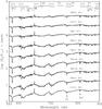 |
Fig. 1 Spectra of Class III YSOs with SpT earlier than M3 in the wavelength region where the spectral classification has been carried out (see text for details). All the spectra are normalized at 750 nm and offset in the vertical direction by 0.5 for clarity. The spectra are also smoothed to the resolution of 2500 at 750 nm to make the identification of the molecular features easier. |
With this spectral typing procedure, we classified all the objects in our sample with SpT earlier than M8. The agreement between the SpTs derived here and those in the literature is good, with only three cases where the difference is two spectral subclasses. We assume the SpT available from the literature for the two YSOs with SpT later than M8 (Reid et al. 2008; Kirkpatrick et al. 2008), because the classification by comparing molecular bands depth with other spectra in the sample is not possible because our sample has a gap between M6.5 and M9. We can only confirm that these objects have a SpT later than the other targets in the sample and that their SpT differ by 0.5 subclass. The SpT obtained here are listed in Table 3 and in the first column of Table 4, and they are used for the rest of the analysis. The distribution of SpT for the sample is shown in Fig. 4. The range of the M-type is almost entirely covered, providing a good sample for the goals of this paper and a solid library of templates that can be used for Lacc estimates of Class II YSOs.
In Appendix B the NIR and UVB spectra of all the sources are shown. Also in these cases a trend with SpT can be seen.
3.2. Spectral indices for M3−M8 stars
Spectral indices provide a fast method of determining SpT for large samples of objects. Here we test some of these indices for M-type objects. Riddick et al. (2007) tested and calibrated various spectral indices in the VIS part of the spectrum for pre main sequence (PMS) stars with SpT from M0.5 to M9. In fact, they suggest using some reliable spectral indices that are valid in the range M3−M8. We find that the best SpT classification can be achieved by combining results obtained using the set of indices that we report in Table 5. We proceeded as follows. For each object we calculated the SpT with all these indices, and then assigned the mean SpT using those results that are in the nominal range of validity of each index. Typical dispersions of the SpT derived with each index are less than half a subclass. We report the final results obtained with these indices in the second column (VIS_ind) of Table 4. Comparing these results with those derived in the previous section, we report an agreement within one subclass for all the objects in the range M3−M8, as expected. However, there are four YSOs classified M1−M2 from the depth of molecular bands that would be classified M3 from the values of the Riddick’s indices. This suggests that spectral classification M3 obtained with spectral indices could, in fact, be earlier by more than one subclass.
There are also indices based on features in the NIR part of the spectrum (e.g. Testi et al. 2001; Testi 2009; Allers et al. 2007; Rojas-Ayala et al. 2012). In Appendix B we compare the results obtained with these NIR indices with the SpT derived in the previous section to confirm the validity of some of these indices for the classification of M-type YSOs.
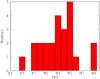 |
Fig. 4 Distribution of spectral types of the Class III YSOs discussed in this work. Each bin corresponds to one spectral subclass. |
Stellar parameters derived for the objects in our sample.
Spectral indices from Riddick et al. (2007, and reference therein) adopted in our analysis for spectral type classification.
4. Stellar parameters
To estimate the mass (M∗), radius (R∗) and age for each target we compare the photospheric parameters (L∗, Teff) with the theoretical predictions of the Baraffe et al. (1998) PMS evolutionary tracks. We derive the Teff of each star from its SpT using the Luhman et al. (2003) SpT− Teff scale, while the procedure for estimating L∗ is described in the next paragraph. We then use (L∗, Teff) to place the stars on the HR diagram and estimate (M∗, age) by interpolating the theoretical evolutionary tracks. These parameters are reported in Table 3. Finally, we obtain R∗ from L∗ and Teff.
4.1. Stellar luminosity
Given the broad wavelength coverage (~300−2500 nm) of the X-shooter spectra, for objects with 2300 < Teff < 4400 K only a low percentage of the stellar flux (≲10−30%) arises from spectral regions outside the X-shooter spectral range. We use, therefore, the following procedure to estimate the total flux of our objects: first, we integrate the whole X-shooter spectrum from 350 nm to 2450 nm, excluding the last 50 nm of spectra on each side, which are very noisy, and the regions in the NIR between the J, H and K-bands (λλ 1330−1550 nm, λλ 1780−2080 nm, see Sect. 2), where we linearly interpolate across the telluric absorption regions. We then use the BT-Settl synthetic spectra from Allard et al. (2011) with the same Teff as our targets (see Table 3), assuming log g = 4.0, which is typical of low-mass YSOs, and normalized with our spectra at 350 and 2450 nm to estimate the contribution to the total flux emitted outside the observed range. The match of the normalization factors at the two ends is very good in all cases. We show in Fig. 5 an example of this procedure.
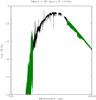 |
Fig. 5 Example of the combination of a flux-calibrated and telluric removed X-shooter spectrum (black) with model spectra with the same Teff (green), which is normalized at the red and blue edges of the X-shooter spectrum and only shown outside the X-shooter range. The telluric bands in the NIR are replaced with a linear interpolation (red). In this figure we show the example of TWA14. |
The main source of uncertainty in L∗ comes from the uncertainty in the spectroscopic flux. For the objects observed in excellent weather conditions, this matches the fotometric fluxes to better than a factor ≲1.5. It is then reasonable to assume such an uncertainty for all the objects in our sample, after normalizing the spectroscopic flux to the photometry (see Sect. 2). This would lead to an uncertainty of less than 0.2 dex in log L∗.
To convert the bolometric fluxes obtained in this way in L∗ we adopt these distances: we assume that YSOs in the σ Ori region have a distance of 360 pc (Brown et al. 1994), those in TW Hya the distances listed in Weinberger et al. (2013), in Torres et al. (2008), and in Mamajek (2005), and those in Lupus III of 200 pc (Comerón 2008), as reported in Table 1. The derived stellar luminosities are listed in Table 3. These values are comparable to those obtained with photometric data in the literature, with a typical difference ≲0.2 dex. As a result, they are consistent with our determinations, within the errors.
4.2. Stellar mass and age
In Fig. 6 we show the Hertzsprung-Russell diagram (HRD) of our PMS stars, built using Teff as reported in Table 3 and L∗ derived in Sect. 4.1. We assign M∗ and age to our PMS stars by interpolating evolutionary tracks from Baraffe et al. (1998) in the HRD. The resulting M∗ are reported in Table 3. For four objects (Sz107, Sz121, TWA26, and TWA29) the position in the HRD implies an age <1 Myr, where theoretical models are known to be very uncertain and, in fact, are typically not tabulated (Baraffe et al. 1998). We estimate the mass of these objects by extrapolating from the closest tabulated points, but we warn the reader that the values are affected by high uncertainty.
Our YSOs are distributed along different isochrones; Lupus YSOs appear to be younger than the others (age ≲ 2 Myr), while σ Ori YSOs are distributed in isochronal ages in the range 2 ≲ age ≲ 10 Myr; finally, TW Hya targets appear generally close to the 10 Myr isochrone. This is in general agreement with what is found in the literature; indeed, Lupus has an estimated age of ~1−1.5 Myr (Hughes et al. 1994; Comerón 2008), while the σ Ori region is usually considered to be slightly older (~3 Myr in average), and ranges from ≲1 Myr to several Myr (Zapatero Osorio et al. 2002; Oliveira et al. 2004). For the TW Hya association, the age estimates are ≳10 Myr (Mamajek 2005; Barrado Y Navascués 2006; Weinberger et al. 2013).
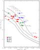 |
Fig. 6 Hertzsprung-Russell Diagram of the Class III YSOs of this work. Data points are compared with the evolutionary tracks (dotted lines) by Baraffe et al. (1998). Isochrones (solid lines) correspond to 2, 10, 30, and 100 Myr. |
5. Line classification
The spectra of our objects are characterized by photospheric absorption lines that depend on the SpT and, in some cases, on the age. To assess the PMS status of the objects in our sample, we check that the lithium absorption feature at λ 670.8 nm, which is related to the age of the YSOs (e.g. Mentuch et al. 2008), is detected in all but one (Sz94) of the objects. We discuss in more detail the implications of the nondetection in Sz94 in Appendix A, and we explain why this object could be considered in our analysis as YSO anyway. The values of the lithium equivalent width (EWLiI) for the other objects in the sample are ~0.5 Å. A detailed analysis of this line and the other photospheric absorption lines of the objects in our sample will be carried out by Stelzer et al. (in prep.).
In addition to these, we detect many emission lines, typically H, He, and Ca lines, that originate in the chromosphere of these stars. In this work we concentrate on the emission lines characterization, since we are interested in the chromospheric activity.
5.1. Emission lines identification
To understand the contribution of the chromospheric emission to the estimate of Lacc through the luminosity of accretion-related emission lines, we first identified in our spectra the lines typically related to accretion processes in Class II YSOs. Here, we describe which lines we detected and report their fluxes and equivalent widths in Tables 6 and 7.
The most common line detected in YSOs is the Hα line at 656.28 nm, which is present in the spectra of all our objects. Emission in this line has been used as a proxy for YSO identification and has been related to accretion processes (e.g. Muzerolle et al. 1998a,b; Natta et al. 2004). This line is also generated in chromospherically active YSOs (e.g. White & Basri 2003). Similarly, the other hydrogen recombination lines of the Balmer series are easily detected in almost all of our Class III objects up to the H12 line (λ 374.9 nm). It is not easy, nevertheless, to determine the continuum around Balmer lines beyond the H9 line (λ 383.5 nm), and the Hϵ line (λ 397 nm) is blended with the CaII-K line. An example of a portion of the spectrum from Hβ to H12 is shown in Fig. 7.
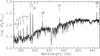 |
Fig. 7 Portion of the spectrum, showing emission in all Balmer lines from Hβ up to H12, as well as the CaII H and K lines, of the YSO TWA13B. The spectrum has been smoothed to a resolution R = 3750 at 375 nm. |
The hydrogen recombination lines of the Paschen and Brackett series, in particular the Paβ (λ 1281.8 nm) and Brγ (λ 2166 nm) lines, have been shown to be related to accretion by Muzerolle et al. (1998a,b). These lines have subsequently been used to survey star forming regions with high extinction (Natta et al. 2004, 2006) in order to obtain accretion rate estimates for VLM objects. We do not detect any of these lines in our Class III spectra, confirming that chromospheric activity is not normally detectable with these lines.
The calcium II emission lines at λλ 393.4, 396.9 nm (Ca HK) and at λλ 849.8, 854.2, 866.2 nm (Ca IRT) are related to accretion processes (e.g. Mohanty et al. 2005; Herczeg & Hillenbrand 2008; Rigliaco et al. 2012), but also to chromospheric activity (e.g. Montes 1998). The CaII H and K lines are detected in 90% of our objects. The CaII IRT lines are detected in 11 out of 13 objects with SpT earlier than M4. These emission lines appear as a reversal in the core of the photospheric absorption lines. For all 11 objects with SpT M4 or later, the CaII IRT lines are not detected.
The HeI line at λ 587.6 nm is also known to be associated with accretion processes (Muzerolle et al. 1998a,b; Herczeg & Hillenbrand 2008), but in Class III YSOs it is known to be of chromospheric origin (e.g. Edwards et al. 2006). The line is indeed detected in 22 (92%) objects. Other HeI lines at λλ 667.8, 706.5, and 1083 nm are usually associated with accretion processes (Muzerolle et al. 1998a,b; Herczeg & Hillenbrand 2008; Edwards et al. 2006). We detect only in Sz122 the HeI lines at λλ 667.8, 706.5 nm, while we detect in 8 (33%) of the objects the HeI line at λ 1083 nm.
Finally, there is no trace of forbidden emission lines in any of our X-shooter spectra, consistent with the expected absence of circumstellar material in Class III YSOs.
5.2. Hα equivalent width and 10% width
A commonly used estimator for the activity in PMS stars is the EW of the Hα line (e.g. White & Basri 2003). This is useful especially when dealing with spectra that are not flux-calibrated or with narrow-band photometric data. The absolute values of this quantity as a function of the SpT of the objects are plotted in Fig. 8, and the values are reported in Table 6. We observe a well-known dependence of EWHα with SpT that is due to decreasing continuum flux for cooler atmospheres. With respect to the threshold to distinguish between accreting and nonaccreting YSOs proposed by White & Basri (2003), all our targets satisfy the criteria of White & Basri (2003) for being nonaccretors.
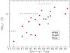 |
Fig. 8 Hα equivalent width as a function of spectral type. The dashed lines represent the boundary between accretors and nonaccretors proposed by White & Basri (2003) for different SpT. |
Another diagnostic to distinguish between accreting and nonaccreting YSOs is the full width of the Hα line at 10% of the line peak (White & Basri 2003). This diagnostic has been shown to be correlated with Ṁacc, but with a large dispersion (Natta et al. 2004). Figure 9 shows the EWHα absolute values versus the 10% Hα width. We see that for most of our objects the 10% Hα width is in the ~100−270 km s-1 range, and for only three objects this value is significantly above the threshold suggested by White & Basri (2003) of 270 km s-1 (TWA6, Sz122, and Sz121). In Appendix A we discuss these objects, and we explain why TWA6 and Sz121 can be considered in our analysis, while Sz122 should be excluded because it is probably an unresolved binary. This is probably due either to high values of vsini for these objects, which broaden the line profile, or to unresolved binarity. For BDs, the threshold for distinguishing accretors from nonaccretors is set at values of the 10% Hα width of 200 km s-1 (Jayawardhana et al. 2003). This is satisfied for all the BDs in the sample. The values of 10% Hα width are listed in Table 6.
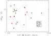 |
Fig. 9 Hα equivalent width as a function of the 10% Hα width. The vertical dashed line rerpesents the White & Basri (2003) criterion for the boundary between accretors and nonaccretors. The objects with 10% Hα width bigger than 270 km s-1 are, from right to left: Sz122, Sz121, TWA6, and TWA13A. |
5.3. Line luminosity
We measure the flux of each line by estimating the continuum in the proximity of the line with the IDL astrolib outlier-resistant mean task resistant_mean. We then subtract the continuum from the observed flux and calculate the integral, checking that the whole line, including the wings, is included in the computation. To compute Lline we adopt the distances reported in Table 3.
For the CaII IRT lines, where the emission appears in the core of the absorption feature, we subtract the continuum from our spectrum following the prescription given by Soderblom et al. (1993). Using a BT-Settl synthetic spectrum (Allard et al. 2011) of the same Teff smoothed at the same resolution of our observed spectrum, we obtain an estimate of the line absorption feature that is then subtracted in order to isolate the emission core of the line; finally, we integrate over the continuum subtracted spectrum. We report in Tables 6 and 7 the values obtained for the fluxes and the line EWs.
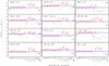 |
Fig. 10 log (Lacc,noise/L⊙) obtained using different accretion tracers and the relations between Lline and Lacc from Alcalá et al. (in prep.). The mean values obtained using the Balmer and HeIλ587.6 lines are shown with the blue solid lines, and the 1σ dispersion is reported with the blue dashed lines. Upper limits are reported with red empty triangles. The 10% Hα width is reported with a blue filled circle. |
We include in Table 6 the values of the observed Balmer jump, defined as the ratio between the flux at ~360 nm and at ~400 nm. Typical values found in the literature for ClassIII YSOs range between ~0.3 and 0.5 (Herczeg & Hillenbrand 2008; Rigliaco et al. 2012). In ClassII YSOs, instead, the observed Balmer jump values are usually higher, up to ~6 (Hartigan et al. 1991; Herczeg & Hillenbrand 2008; Rigliaco et al. 2012). For the objects in our sample, this quantity ranges between ~0.35 and ~0.55 (see Table 6), with the exception of Sz122. The values of the Balmer jump ratio for the three BDs in the sample are not reported, because the S/N of the UVB spectrum of these sources is too low to estimate this quantity.
6. Implications for mass accretion rates determination
The physical parameter that is used to estimate the accretion activity in Class II YSOs is
Ṁacc, which is derived from Lacc
and the stellar parameters using the following relation (Hartmann et al. 1998): 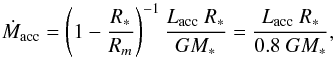 (1)where the factor 0.8 is due
to the assumption that the accretion flows arise from a magnetospheric radius
Rm ~ 5 R∗ (Shu et al. 1994).
(1)where the factor 0.8 is due
to the assumption that the accretion flows arise from a magnetospheric radius
Rm ~ 5 R∗ (Shu et al. 1994).
When estimating Lacc in Class II YSOs with the direct method of UV-excess fitting (e.g. Valenti et al. 1993), the contribution to the continuum excess emission due to chromospheric activity is probably negligible, and it is normally taken into account using a Class III YSO of the same SpT as a template for the analysis (e.g. Herczeg & Hillenbrand 2008; Rigliaco et al. 2011, 2012). However, Lacc is often derived using spectral lines luminosity and appropriate empirical relations (see e.g. Muzerolle et al. 1998a,b; Natta et al. 2004; Herczeg & Hillenbrand 2008, and references therein). Several of the lines normally used for these studies are influenced by chromospheric activity (Sect. 5), which should be estimated and subtracted from the line emission before computing Lacc. This procedure is not trivial, since it is difficult to properly disentangle the two emission processes in each object and each line. All the Lacc − Llines relations are always based on the uncorrected values of Lline. This correction, as shown in Ingleby et al. (2011) and Rigliaco et al. (2012), can be important in objects with low Lacc and, in particular, in VLM stars. Therefore, the chromospheric emission acts as a systematic “noise" that affects the Lacc measurements.
In the following, we characterize this effect using the Lline derived in Sect. 5 and the most recent Lacc − Lline relations for Class II YSOs derived by Alcalá et al. (in prep.). These relations have been derived using the same method as described in Rigliaco et al. (2012), where Laccis obtained from the continuum excess emission and then compared with the Llineof the several emission line diagnostics in every object. In Alcalá et al. (in prep.) the sample is composed of 36 YSOs located in the Lupus-I and Lupus-III clouds, together with eight additional YSOs located in the σ-Ori region from Rigliaco et al. (2012). These relations are not quantitatively different from those in the literature, but have significantly smaller uncertainties and have been derived for stars with similar properties than the Class III analyzed here. For each Class III object, we compute Lacc from a number of different lines, as described in the following. This provides a measurement of the “noise” introduced in the determination of Lacc from line luminosities in Class II. It represents a typical threshold for determining Lacc in Class II objects by chromospheric activity, assuming that this is approximately the same in the two different classes of objects, with and without ongoing accretion. We define it in the following as Lacc,noise.
6.1. Accretion luminosity noise
Alcalá et al. (in prep.) use a sample of Class II YSOs in the Lupus star forming region observed with X-shooter to refine the Lacc − Lline relations. We adopt their relations to estimate the Lacc,noise for our Class III YSOs, using in particular the Hα, Hβ, Hγ, Hδ, H8, H9, H10, H11, HeI (λλ587.6, and 1083 nm), CaII (λ393 nm), CaII (λ849.8 nm), CaII (λ854.2 nm), and CaII (λ866.2 nm) lines. Moreover, we use the relation from Natta et al. (2004) between Ṁacc and the 10% Hα width to estimate Lacc,noise from this indicator.
We show in Fig. 10−11 the values of Lacc,noise for every object obtained using the different indicators. The uncertainties on these values are dominated by the errors in the relations between Lline and Lacc. Upper limits for undetected lines indicate the 3σ upper limits. Each Balmer line leads to values of Lacc,noise that always agree with the other Balmer lines by less than ~0.2 dex, and similarly the HeIλ587.6 line almost in all cases. The HeIλ1083 and the CaII lines, instead, in various cases do not agree with the result obtained using the Balmer and HeIλ587.6 lines, with differences even larger than 0.6 dex. It should be considered that the exact value of the CaII IRT lines luminosity is subject to many uncertainties, owing to the complicated procedure for estimating the excess luminosity (see Sect. 5.3).
The Paschen and Brackett HI emission lines are not detected in our spectra, as pointed out in Sect. 5.1. We report in Figs. 10−11 the 3σ upper limits for Lacc,noise obtained using the Paβ and Brγ line luminosities and the relations from Alcalá et al. (in prep.). These values are always below the mean Lacc,noise value obtained with the Balmer and HeIλ587.6 lines. This implies that those lines are less sensitive to chromospheric activity than the Balmer lines.
The 10% Hα width is the accretion indicator that leads to values of Lacc,noise that are more discrepant from the mean (Figs. 10, 11). This clearly does not follow in more than 50% of the cases the results obtained using the other indicators. This is not surprising since the Hα width is mainly a kinematics measurement, unlike Lline measurements. It is to be expected that the application of a method calibrated for accretion processes to chromospheric activity would result in inconsistencies. We know that the broadening of the Hα line and the other accretion-related lines is due to the high-velocity infall of material in the accretion flows, while the intensity of the emission lines is due to emission from the high-temperature region. The latter can be either accretion shocks on the stellar surface or chromospheric emission. That in our sample of nonaccreting objects relations converting Lline to Lacc lead to similar results when using line fluxes, while the result is quite different when using line broadening seems to confirm that the Hα 10% width we detect is only due to thermal broadening in the chromosphere of these stars and not to the gas flow kinematics associated with the accretion onto the central object.
For all objects, the mean Lacc,noise value
is always below ~10-3 L⊙, and this value decreases
monotonically with the SpT. In Fig. 12 these mean
values of
log (Lacc,noise/L⊙)
obtained with the Balmer and HeIλ587.6 lines are plotted as a
function of the Teff of the objects. The error bars on the
plot represent the standard deviation of the derived values of
Lacc,noise3. These values should be intended as the noise in the
Lacc values arising from the chromospheric activity. In Fig.
13 we show the mean values of the logarithmic
ratio
Lacc,noise/L∗
obtained using the Balmer and HeIλ587.6 lines as a function of
the Teff. Unlike Fig. 12, the quantity
Lacc,noise/L∗ is unbiased by
uncertainties on distance values or by different stellar ages, leading to smaller spreads.
We see that from the K7 objects down to the BDs, the values of
log(Lacc,noise/L∗)
decrease with the Teff of the YSOs. After fitting the
Lacc,noise–
Teff relation with a powerlaw, using only the objects in the
range K7−M9.5, and excluding Sz122 (see Appendix A
for details), we obtain the following analytical relation (Fig. 13):  (2)The only clear
deviation from the general trend, apart from Sz122, is the K5 YSO TWA9A, which shows a
value of
log (Lacc,noise/L∗)
lower by ~0.6 dex with respect to what should be expected by the extrapolation of the
previous relation. Unfortunately, our sample is too small, and we do not have other
objects with earlier SpT to verify whether this low value is actually a different trend
due to different chromospheric activity for earlier SpT YSOs or if the source is peculiar.
There are also signatures of different chromospheric activity intensity among objects with
the same SpT and located in the same region; for example, the two TW Hya M1 YSOs, which
are two components of a binary system, thus coeval objects, have a spread in
log (Lacc,noise/L∗)
of ~0.5 dex.
(2)The only clear
deviation from the general trend, apart from Sz122, is the K5 YSO TWA9A, which shows a
value of
log (Lacc,noise/L∗)
lower by ~0.6 dex with respect to what should be expected by the extrapolation of the
previous relation. Unfortunately, our sample is too small, and we do not have other
objects with earlier SpT to verify whether this low value is actually a different trend
due to different chromospheric activity for earlier SpT YSOs or if the source is peculiar.
There are also signatures of different chromospheric activity intensity among objects with
the same SpT and located in the same region; for example, the two TW Hya M1 YSOs, which
are two components of a binary system, thus coeval objects, have a spread in
log (Lacc,noise/L∗)
of ~0.5 dex.
Values of Lline and Lacc in Class II YSOs that are close to those estimated in this work should be considered very carefully, because the chromospheric activity could be an important factor in the excess luminosity in the line and could produce misleading results.
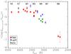 |
Fig. 12 Mean values of log (Lacc,noise/L⊙) obtained with different accretion diagnostics as a function of Teff. Error bars represent the standard deviation around the mean log (Lacc,noise/L⊙). These data should be intended as the noise in the values of Lacc due to chromospheric emission flux. |
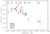 |
Fig. 13 Mean values of log (Lacc,noise/L∗) obtained with different accretion diagnostics as a function of log Teff. The dashed line is the best fit to the data, whose analytical form is reported in Eq. (2). Two objects (Sz122 and TWA9A) are excluded from the fit (empty symbols), as explained in the text. |
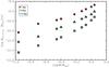 |
Fig. 14 log Ṁacc,noise as a function of log M∗, with values of Ṁacc,noise obtained using three different isochrones from Baraffe et al. (1998) and the values of Lacc,noise/L∗ derived from the fit in Eq. (2) at any Teff. Results using the 1 Myr isochrone are reported with filled circles, those using the 3 Myr isochrone with filled triangles, and those using the 10 Myr isochrone with filled squares. |
6.2. Mass accretion rate noise
In this section, we determine what the typical “chromospheric noise” on Ṁacc would be when derived from indirect methods if the chromospheric emission is not subtracted before computing Lline. We refer to this quantity as Ṁacc,noise.
The procedure is the following. We select three isochrones (1, 3, and 10 Myr) from Baraffe et al. (1998) models and nine different YSOs masses (0.11, 0.20, 0.35, 0.40, 0.60, 0.75, 0.85, 1.00, and 1.10 M⊙), which always correspond to Teff in the range 2500−4000 K, where our results are applicable. Then, for each Teff we derive Lacc,noise/L∗ using the fit reported in Eq. (2). Finally, we use Eq. (1), adopting the proper R∗, M∗, and L∗ at any age from the Baraffe et al. (1998) tracks, in order to determine the typical Ṁacc,noise at different ages as a function of M∗. The results are shown in Fig. 14, where a strong correlation between the two parameters is evident, with increasing Ṁacc,noise with M∗. At the same time, the variation in Ṁacc,noise with age at any given M∗ is large, up to 0.5 dex for differences of 2 Myr at the H-burning limit, but decreases with increasing M∗. Similar results are obtained when using other evolutionary models.
We derive a limit on the detectable Ṁacc of ~6.6 × 10⁻¹⁰ M⊙/yr for solar-mass, young (1 Myr) objects, decreasing to 2.5 × 10⁻¹²M⊙/yr for low-mass, older (10 Myr) objects. We report these Ṁacc,noise values for the three isochrones analyzed in Table 8.
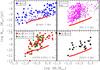 |
Fig. 15 log Ṁacc as a function of log M∗ for Class II objects located in different star forming regions. Data for ρ Oph are from Natta et al. (2006), corrected for new distance measurements by Rigliaco et al. (2011); ONC points are from Manara et al. (2012), data for L1630N and L1641 are from Fang et al. (2009), and those for ChaII from Biazzo et al. (2012). Ṁacc values obtained with indirect methods are shown with colored, filled points, while measurements based on the direct U-band excess method are shown with gray empty points as a reference. Downwards triangles refer to upper limits. The thick red solid line is the lower limit to the measurements of Ṁacc set by chromospheric activity in the line emission. We use the values for the correct isochrone according to the mean value of the age for each region, as reported on the plot. |
Values of log Ṁacc,noise at different M∗ and ages.
6.2.1. Comparison with literature data
As discussed, Ṁacc,noise is a lower limit to the values of Ṁacc that can be derived from the luminosity of lines emitted by stellar chromospheres. In this section, we compare this chromospheric limit with estimates of Ṁacc based on Lline from the literature. We show in Fig. 15 values of Ṁacc as a function of M∗ obtained with optical or NIR emission lines as accretion diagnostic for objects located in four star forming regions with different ages: ρ-Ophiucus, the Orion Nebula Cluster, the L1630N and L1641 regions, and the Chameleon II region. We overplot the locii of Ṁacc,noise obtained using the proper isochrone for the mean age of each region. In this way we do not address possible differences in Ṁacc due to age spreads in these regions, but these spreads, if present, are ≲1−2 Myr (see e.g. Reggiani et al. 2011). The effect of a similar age spread on the Ṁacc,noise threshold would be ~0.5 dex for low-mass objects and ~0.3 dex for solar-mass stars (see Fig. 14).
We consider in this analysis Ṁacc values obtained using optical emission lines. In Fig. 15 we show the values for the ~1 Myr old regions L1630N and L1641 (Fang et al. 2009), where the Hα, Hβ, and HeI lines were used, those for the ~2−3 Myr old Orion Nebula Cluster (Manara et al. 2012) obtained with photometric narrow-band Hα luminosity estimates4, and those obtained with the Hα, Hβ, and HeI lines for the ~4 Myr old Chameleon II region (Biazzo et al. 2012). In all these cases, the vast majority of datapoints are found, as expected, well above the Ṁacc,noise threshold, confirming that the chromospheric contribution to the line emission is negligible for strongly accreting YSOs. Nevertheless, there are a few (11) objects in L1630N and L1641, where measured values of Ṁacc are lower than the expected Ṁacc,noise. One possibility to explain this result is variable accretion in these objects, which has been found to vary as much as 0.4 dex on time scales of one year (Costigan et al. 2012). Still, this does not explain why only lower mass objects happen to be below the threshold. In any case, these points should be considered with caution, since the measured Lline could be completely due to chromospheric emission, leading to erroneous estimates of Ṁacc.
For the ~1 Myr old ρ Ophiucus region we consider the Lline derived through Paβ and Brγ lines (Natta et al. 2006), corrected for a more recent estimate of the distance (see Rigliaco et al. 2011). As we noted in Sects. 5.1 and 6.1, Paβ and Brγ lines are not detected in our Class III YSOs spectra. In Fig. 15, all the detections are located well above the Ṁacc,noise locus, while the upper limits are distributed also at the edge of the Ṁacc,noise threshold. This confirms the validity of these NIR lines as good tracers of accretion and the fact that they are most likely less subject to chromospheric noise than the Balmer and HeIλ587.6 lines.
7. Conclusion
In this paper, we presented the analysis of 24 diskless, hence nonaccreting, Class III YSOs, observed with the broad-band, medium-resolution, high-sensitivity VLT/X-shooter spectrograph. The targets are located in three nearby star forming regions (Lupus III, σ Ori, and TW Hya) and have SpT in the range from K5 to M9.5. We checked the SpT classifications, using both spectral indices and broad molecular bands. Moreover, using the flux calibrated spectra, we derived the stellar luminosity. Then, we analyzed the emission lines related to accretion processes in accreting objects that are present in these spectra and, from their luminosities, we studied the implications of chromospheric activity for Ṁacc determination in accreting (Class II) objects. This was done by deriving the parameter Lacc,noise, which is the systematic “noise” introduced by chromospheric emission in the measurements of Lacc from line emission in Class II objects. For this analysis we assumed a similar chromospheric activity in the two classes of objects.
Our main conclusions are:
-
1.
All hydrogen recombination emission lines of the Balmerseries are detected in our sample of Class III YSOsspectra when the S/N is high enough. In contrast, Paschen andBrackett series lines are not detected in emission, and they aresignificantly weaker, when compared to Balmer lines, than inClass II objects. The chromospheric “noise” inthese lines is lower than in the optical lines (seeFigs. 10, 11), and they are verygood tracers of accretion in low-mass, low accretion rate objects.
-
2.
Using Balmer and HeIλ587.6 lines and the calibrated relations between Lline and Lacc from the literature, we derived Lacc,noise values that always show good agreement among all the lines.
-
3.
Calcium emission lines in the NIR spectral range (λλ 849.8, 854.2, 866.2 nm) are detected in 11 objects (45% of the sample) superposed on the photospheric absorption lines. This results in a more complicated line flux measurement than for other lines. Their behavior with respect to the hydrogen line luminosities is different; in particular, the values of Lacc,noise obtained using these lines often do not agree well with those obtained using Balmer and HeIλ587.6 lines.
-
4.
The mean values of Lacc,noise for the objects in our sample are lower than ~10-3 L⊙ and have a clear dependence with Teff for K7−M9.5 objects. Therefore, Lacc of this order or smaller measured in Class II objects using line luminosity as a proxy of accretion may be significantly overestimated if the chromospheric contribution to the line luminosity is not taken into account.
-
5.
Our results show that the “noise” due to chromospheric activity on the estimate of Ṁacc in Class II YSOs obtained using secondary indicators for accretion has a strong dependence on M∗ and age. Typical values of log(Ṁacc,noise) for M-type YSOs are in the range from ~−9.2 for solar-mass young (1 Myr) objects to −11.6 M⊙/yr for low-mass, older (10 Myr) objects. Therefore, derived accretion rates below this threshold should be treated with caution because the line emission may be dominated by chromospheric activity.
Online material
Fluxes and equivalent widths of Balmer lines.
Fluxes and equivalent widths of helium and calcium lines.
Appendix A: Comments on individual objects
Appendix A.1: Sz94
Sz94 was discovered as an Hα emitting star in the survey by Schwarz (1977). Since then, it has been considered as a PMS star in reviews and investigations (Krautter 1992; Hughes et al. 1994; Comerón 2008; Mortier et al. 2011), but nothing has been mentioned about the presence of the lithium absorption line at 670.8 nm. Based on its spectral energy distribution, Sz94 has been classified as a Class III IR YSO by Merín et al. (2008). For all these reasons, we included the star in our program as a Class III template of M4 SpT. Notwithstanding the high quality of the X-shooter data in terms of S/N and resolution, the Li I λ 670.8 nm line is not present in the spectrum, and we determine an upper limit of EWLi < 0.1 Å. The question then rise whether lithium may have already been depleted in the star. However, lithium is significantly depleted by large factors only after several tens of Myr, inconsistently with the average age of a few Myr of the Lupus members. Analysis of the radial velocity of this object shows that its value is in the typical range for Lupus sources Stelzer et al. (in prep.). We consider here the source as a PMS, given its position in the HRD, the Hα emission, and the radial velocity measurement, but more analysis should be done to confirm its PMS status.
Appendix A.2: Sz122
Sz122 is a Class III object classified with Spitzer (Merín et al. 2008). All the lines of this object appear very broadened. Nevertheless, the spectrum cannot be fitted with synthetic spectra broadened at reasonable values of vsini, meaning that this is not a single fast rotator. We think, therefore, that this object is a binary system. This could explain the very faint LiI line (EWLi < 0.25 Å) and the lack of emission in the CaII IRT absorption features, which is usually found in other early M-type objects of our sample. Even the presence of a broad Hα line (10% width >600 km s-1) can be explained by the presence of two objects. We do not consider this object in the analysis of the implications of chromospheric activity on Ṁacc measurements, because the effect of its binarity cannot be accounted for.
Appendix A.3: Sz121
Similar to Sz122, the lines of this object appear very broadened. Also in this case, the object is classified with Spitzer as a Class III (Merín et al. 2008). We can fit the spectrum with a synthetic spectrum of the same Teff, log g = 4.0, and vsini = 70 km s-1. This value of vsini is rather high for a typical M4-type YSO. If true, it would be an extreme ultrafast rotator. The large 10% Hα width (~380 km s-1) is then due to its very high rotational velocity. Another possibility is that this object may also be an unresolved spectroscopic binary.
Appendix A.4: TWA6
This object has been discovered and classified as a young nonaccreting object by Webb et al. (1999). It is a member of the TWA association, and it is a known fast rotator (vsini = 72 km s-1, Skelly et al. 2008). We measure a 10% Hα width of 362 km s-1. This is larger than the threshold to distinguish the accreting and nonaccreting objects proposed by White & Basri (2003). Nevertheless, this object can be considered a Class III YSO for the small EWHα, the small Balmer jump, and in particular, the IR classification. For these reasons we consider this object in our analysis.
Appendix B: NIR spectral indices
Spectral indices in the NIR part of the spectrum are particularly useful for classifying VLM stars and BDs, which emit most of their radiation in this spectral region. Therefore, various analyses to calibrate reliable NIR indices to classify late M-type objects and BDs have been carried out in the past (e.g. Kirkpatrick et al. 1999). With our sample, we are able to verify the validity of various NIR indices for M-type YSOs, comparing the SpT obtained through optical spectroscopy (Sect. 3). We consider in this analysis different NIR indices that have been calibrated using either dwarfs or young stars (subgiants) for objects with SpT M or later. In particular, Rojas-Ayala et al. (2012) calibrated the H2O−K2 index using a sample of M dwarfs, and derived a relation valid for the whole M class. Allers et al. (2007) calibrated the gravity-independent spectral index H2O on a sample of young BDs and dwarfs. This is valid for objects with SpT in the range M5−L0. Testi et al. (2001) and Testi (2009) proposed various spectral indices (sH2OJ, sH2OK, sKJ, sHJ, sH2OH1, sH2OH2, IJ, IH, and IK) to classify M-, L-, and T-type BDs, calibrating those on a large sample of dwarfs; finally, Scholz et al. (2012) used a sample of VLM YSOs to calibrate the HP index, which is valid for objects with SpT in the range M7−M9.5. We report those indices in Table B.1.
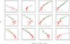 |
Fig. B.1 Spectral type of the objects as a function of the spectral index values obtained with different NIR indices (Table B.1). Red symbols are values from this work, while green crosses are from Testi et al. (2001) and Testi (2009). Red stars are used for objects with SpT in the range of validity of the index, while red pentagons for those not in the range of validity of the index. Dashed lines are the best fit from the reference cited in Table B.1 for each index, when available. No published relations are available for the indices IJ and IK. Black and red solid lines are the best fits (black = linear, red = polynomial) from this work, considering both our sample and the values from the literature. |
Figure B.1 shows the results of this analysis. The SpTs obtained in Sect. 3 are reported as a function of each spectral index for our objects. For the spectral indices derived in Testi et al. (2001) and Testi (2009), we report also the data for the sample of L- and M-type dwarfs they adopted in the analysis. We stress that the latter sample should be considered with caution, since gravity dependent spectral indices calibrated using samples of dwarfs may not be reliable for YSOs, which are subgiants.
We see that the indices sH2OH2, sKJ, sHJ, and IK cannot be used to classify YSOs of M-type class. In contrast, we find a good correlation with the indices sH2OK, sH2OJ, sH2OH1, IJ, and IH. For these indices we decide to fit our objects and those from the literature together in all cases, using either a linear or a second-degree polynomial fit. We show the best fit obtained in Fig. B.1. Using these relations, we derived the SpT for each of our YSOs, and we report these results in Table 4. We thus propose new SpT-spectral index relations for the following five indices from Testi et al. (2001) and Testi (2009). The first three are valid for objects with SpT later and equal to M1:
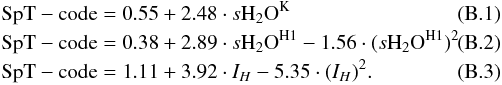 The
following two indices are valid for objects with SpT later and equal to M2:
The
following two indices are valid for objects with SpT later and equal to M2:
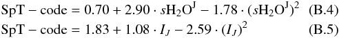 where
the SpT are coded in the following way: M0 ≡ 0.0, M9 ≡ 0.9, L5 ≡ 1.5, and a variation of
0.1 corresponds to a step of one subclass. For these spectral indices we conclude that
results for objects with SpT in the nominal range of validity of each index are reliable
within a typical uncertainty of about one subclass.
where
the SpT are coded in the following way: M0 ≡ 0.0, M9 ≡ 0.9, L5 ≡ 1.5, and a variation of
0.1 corresponds to a step of one subclass. For these spectral indices we conclude that
results for objects with SpT in the nominal range of validity of each index are reliable
within a typical uncertainty of about one subclass.
A good correlation is also found for the spectral index H2O−K2. Using the analytical relation between SpT and spectral index from the literature, we obtain for 13 out of 22 objects with M SpT results that are compatible within one subclass with the correct SpT (see Table 4). The differences can be due to the imperfect telluric removal in the first interval of interest of this index. Moreover, we confirm that the H2O index is valid for YSOs with SpT in the range M5−M9.5, finding agreement
within one subclass for all our objects (see Table 4). Regarding the HP index, we confirm that it is not valid for YSOs with SpT earlier than M7, and we observe that the SpT obtained with this index confirm those from the literature for our two later SpT objects (see Table 4).
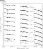 |
Fig. C.1 Spectra of Class III YSOs with spectral type earlier than M3 in the NIR arm. All the spectra are normalized at 1700 nm and offset in the vertical direction by 0.5 for clarity. The spectra are also smoothed to the resolution of 2000 at 2000 nm to make identification of features easier. |
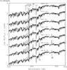 |
Fig. C.4 Spectra of Class III YSOs with spectral type earlier than M2 in the UVB arm. All the spectra are normalized at 450 nm and offset in the vertical direction for clarity. The spectra are also smoothed to the resolution of 1500 at 400 nm to make identification of features easier. |
IRAF is distributed by National Optical Astronomy Observatories, which is operated by the Association of Universities for Research in Astronomy, Inc., under cooperative agreement with the National Science Foundation.
We also report the values of Ṁacc obtained through U-band excess by Manara et al. (2012), which are shown as a comparison.
Acknowledgments
C.F.M. acknowledges the Ph.D. fellowship of the International Max-Planck-Research School. We thank Aleks Scholz, Greg Herczeg, and Luca Ricci for insightful discussions. This research made use of the SIMBAD database and of the VizieR catalog access tool, operated at the CDS, Strasbourg, France.
References
- Alcalá, J. M., Stelzer, B., Covino, E., et al. 2011, Astron. Nachr., 332, 242 [NASA ADS] [CrossRef] [Google Scholar]
- Allard, F., Homeier, D., & Freytag, B. 2011, ASP Conf. Ser., 448, 91 [NASA ADS] [Google Scholar]
- Allen, L. E., & Strom, K. M. 1995, AJ, 109, 1379 [NASA ADS] [CrossRef] [Google Scholar]
- Allers, K. N., Jaffe, D. T., Luhman, K. L., et al. 2007, ApJ, 657, 511 [NASA ADS] [CrossRef] [Google Scholar]
- Baraffe, I., Chabrier, G., Allard, F., & Hauschildt, P. H. 1998, A&A, 337, 403 [NASA ADS] [Google Scholar]
- Barrado Y Navascués, D. 2006, A&A, 459, 511 [NASA ADS] [CrossRef] [EDP Sciences] [Google Scholar]
- Biazzo, K., Alcalá, J. M., Covino, E., et al. 2012, A&A, 547, A104 [NASA ADS] [CrossRef] [EDP Sciences] [Google Scholar]
- Brown, A. G. A., de Geus, E. J., & de Zeeuw, P. T. 1994, A&A, 289, 101 [NASA ADS] [Google Scholar]
- Burningham, B., Naylor, T., Littlefair, S. P., & Jeffries, R. D. 2005, MNRAS, 356, 1583 [NASA ADS] [CrossRef] [Google Scholar]
- Caballero, J. A. 2008, A&A, 478, 667 [NASA ADS] [CrossRef] [EDP Sciences] [Google Scholar]
- Caballero, J. A., Albacete-Colombo, J. F., & López-Santiago, J. 2010, A&A, 521, A45 [NASA ADS] [CrossRef] [EDP Sciences] [Google Scholar]
- Calvet, N., & Gullbring, E. 1998, ApJ, 509, 802 [NASA ADS] [CrossRef] [Google Scholar]
- Cieza, L., Padgett, D. L., Stapelfeldt, K. R., et al. 2007, ApJ, 667, 308 [NASA ADS] [CrossRef] [Google Scholar]
- Comerón, F. 2008, Handbook of Star Forming Regions, 42, 295 [Google Scholar]
- Comerón, F., Fernández, M., Baraffe, I., Neuhäuser, R., & Kaas, A. A. 2003, A&A, 406, 1001 [NASA ADS] [CrossRef] [EDP Sciences] [Google Scholar]
- Costigan, G., Scholz, A., Stelzer, B., et al. 2012, MNRAS, 427, 1344 [NASA ADS] [CrossRef] [Google Scholar]
- Cutri, R. M., Skrutskie, M. F., van Dyk, S., et al. 2003, VizieR Online Data Catalog, II/246 [Google Scholar]
- Da Rio, N., Robberto, M., Soderblom, D. R., et al. 2010, ApJ, 722, 1092 [NASA ADS] [CrossRef] [Google Scholar]
- DENIS Consortium 2005, VizieR Online Data Catalog, II/263 [Google Scholar]
- Edwards, S., Fischer, W., Hillenbrand, L., & Kwan, J. 2006, ApJ, 646, 319 [NASA ADS] [CrossRef] [Google Scholar]
- Fang, M., van Boekel, R., Wang, W., et al. 2009, A&A, 504, 461 [NASA ADS] [CrossRef] [EDP Sciences] [Google Scholar]
- Fedele, D., van den Ancker, M. E., Henning, T., Jayawardhana, R., & Oliveira, J. M. 2010, A&A, 510, A72 [NASA ADS] [CrossRef] [EDP Sciences] [Google Scholar]
- Franchini, M., Morossi, C., & Malagnini, M. L. 1998, ApJ, 508, 370 [NASA ADS] [CrossRef] [Google Scholar]
- Gómez, M., & Mardones, D. 2003, AJ, 125, 2134 [NASA ADS] [CrossRef] [Google Scholar]
- Hartigan, P., Kenyon, S. J., Hartmann, L., et al. 1991, ApJ, 382, 617 [NASA ADS] [CrossRef] [Google Scholar]
- Hartmann, L., Calvet, N., Gullbring, E., & D’Alessio, P. 1998, ApJ, 495, 385 [NASA ADS] [CrossRef] [Google Scholar]
- Henry, T. J., Kirkpatrick, J. D., & Simons, D. A. 1994, AJ, 108, 1437 [NASA ADS] [CrossRef] [Google Scholar]
- Herczeg, G. J., & Hillenbrand, L. A. 2008, ApJ, 681, 594 [NASA ADS] [CrossRef] [Google Scholar]
- Hernández, J., Hartmann, L., Megeath, T., et al. 2007, ApJ, 662, 1067 [NASA ADS] [CrossRef] [Google Scholar]
- Høg, E., Fabricius, C., Makarov, V. V., et al. 2000, A&A, 355, L27 [NASA ADS] [Google Scholar]
- Houdebine, E. R., Mathioudakis, M., Doyle, J. G., & Foing, B. H. 1996, A&A, 305, 209 [NASA ADS] [Google Scholar]
- Hughes, J., Hartigan, P., Krautter, J., & Kelemen, J. 1994, AJ, 108, 1071 [NASA ADS] [CrossRef] [Google Scholar]
- Ingleby, L., Calvet, N., Bergin, E., et al. 2011, ApJ, 743, 105 [NASA ADS] [CrossRef] [Google Scholar]
- Jayawardhana, R., Mohanty, S., & Basri, G. 2003, ApJ, 592, 282 [NASA ADS] [CrossRef] [Google Scholar]
- Kenyon, S. J., & Hartmann, L. 1995, ApJS, 101, 117 [NASA ADS] [CrossRef] [Google Scholar]
- Kirkpatrick, J. D., Reid, I. N., Liebert, J., et al. 1999, ApJ, 519, 802 [NASA ADS] [CrossRef] [Google Scholar]
- Kirkpatrick, J. D., Cruz, K. L., Barman, T. S., et al. 2008, ApJ, 689, 1295 [NASA ADS] [CrossRef] [Google Scholar]
- Krautter, J. 1992, Low Mass Star Formation in Southern Molecular Clouds, 127 [Google Scholar]
- Looper, D. L., Burgasser, A. J., Kirkpatrick, J. D., & Swift, B. J. 2007, ApJ, 669, L97 [NASA ADS] [CrossRef] [Google Scholar]
- Luhman, K. L. 2004, ApJ, 602, 816 [NASA ADS] [CrossRef] [Google Scholar]
- Luhman, K. L., Stauffer, J. R., Muench, A. A., et al. 2003, ApJ, 593, 1093 [NASA ADS] [CrossRef] [Google Scholar]
- Gullbring, E., Hartmann, L., Briceno, C., & Calvet, N. 1998, ApJ, 492, 323 [NASA ADS] [CrossRef] [Google Scholar]
- Mamajek, E. E. 2005, ApJ, 634, 1385 [NASA ADS] [CrossRef] [Google Scholar]
- Manara, C. F., Robberto, M., Da Rio, N., Lodato, G., et al. 2012, ApJ, 755, 154 [NASA ADS] [CrossRef] [Google Scholar]
- Mentuch, E., Brandeker, A., van Kerkwijk, M. H., Jayawardhana, R., & Hauschildt, P. H. 2008, ApJ, 689, 1127 [NASA ADS] [CrossRef] [Google Scholar]
- Merín, B., Jørgensen, J., Spezzi, L., et al. 2008, ApJS, 177, 551 [NASA ADS] [CrossRef] [Google Scholar]
- Messina, S., Desidera, S., Tutatto, M., Lanzafame, A. C., & Guinan, E. F. 2010, VizieR Online Data Catalog, 352, 9015 [Google Scholar]
- Modigliani, A., Goldoni, P., Royer, F., et al. 2010, Proc. SPIE, 7737 [Google Scholar]
- Mohanty, S., Jayawardhana, R., & Basri, G. 2005, ApJ, 626, 498 [NASA ADS] [CrossRef] [Google Scholar]
- Montes, D. 1998, Ap&SS, 263, 231 [NASA ADS] [CrossRef] [Google Scholar]
- Morrison, J. E., Röser, S., McLean, B., Bucciarelli, B., & Lasker, B. 2001, AJ, 121, 1752 [NASA ADS] [CrossRef] [Google Scholar]
- Mortier, A., Oliveira, I., & van Dishoeck, E. F. 2011, MNRAS, 418, 1194 [NASA ADS] [CrossRef] [Google Scholar]
- Muzerolle, J., Calvet, N., & Hartmann, L. 1998a, ApJ, 492, 743 [NASA ADS] [CrossRef] [Google Scholar]
- Muzerolle, J., Hartmann, L., & Calvet, N. 1998b, AJ, 116, 455 [NASA ADS] [CrossRef] [Google Scholar]
- Natta, A., Testi, L., Muzerolle, J., et al. 2004, A&A, 424, 603 [NASA ADS] [CrossRef] [EDP Sciences] [Google Scholar]
- Natta, A., Testi, L., & Randich, S. 2006, A&A, 452, 245 [NASA ADS] [CrossRef] [EDP Sciences] [Google Scholar]
- Oliveira, J. M., Jeffries, R. D., & van Loon, J. T. 2004, MNRAS, 347, 1327 [NASA ADS] [CrossRef] [Google Scholar]
- Oliveira, J. M., Jeffries, R. D., van Loon, J. T., & Rushton, M. T. 2006, MNRAS, 369, 272 [NASA ADS] [CrossRef] [Google Scholar]
- Reggiani, M., Robberto, M., Da Rio, N., et al. 2011, A&A, 534, A83 [NASA ADS] [CrossRef] [EDP Sciences] [Google Scholar]
- Reid, I. N., Cruz, K. L., Kirkpatrick, J. D., et al. 2008, AJ, 136, 1290 [NASA ADS] [CrossRef] [Google Scholar]
- Riaz, B., Gizis, J. E., & Harvin, J. 2006, AJ, 132, 866 [NASA ADS] [CrossRef] [Google Scholar]
- Riddick, F. C., Roche, P. F., & Lucas, P. W. 2007, MNRAS, 381, 1067 [NASA ADS] [CrossRef] [Google Scholar]
- Rigliaco, E., Natta, A., Randich, S., Testi, L., & Biazzo, K. 2011, A&A, 525, A47 [NASA ADS] [CrossRef] [EDP Sciences] [Google Scholar]
- Rigliaco, E., Natta, A., Testi, L., et al. 2012, A&A, 548, A56 [NASA ADS] [CrossRef] [EDP Sciences] [Google Scholar]
- Rojas-Ayala, B., Covey, K. R., Muirhead, P. S., & Lloyd, J. P. 2012, ApJ, 748, 93 [NASA ADS] [CrossRef] [Google Scholar]
- Sacco, G. G., Franciosini, E., Randich, S., & Pallavicini, R. 2008, A&A, 488, 167 [NASA ADS] [CrossRef] [EDP Sciences] [Google Scholar]
- Samus’, N. N., Goranskii, V. P., Durlevich, O. V., et al. 2003, Astron. Lett., 29, 468 [NASA ADS] [CrossRef] [Google Scholar]
- Scholz, A., Muzic, K., Geers, V., et al. 2012, ApJ, 744, 6 [NASA ADS] [CrossRef] [Google Scholar]
- Sherry, W. H., Walter, F. M., & Wolk, S. J. 2004, AJ, 128, 2316 [NASA ADS] [CrossRef] [Google Scholar]
- Shkolnik, E. L., Liu, M. C., Reid, I. N., Dupuy, T., & Weinberger, A. J. 2011, ApJ, 727, 6 [NASA ADS] [CrossRef] [Google Scholar]
- Shu, F. H., Adams, F. C., & Lizano, S. 1987, ARA&A, 25, 23 [Google Scholar]
- Shu, F., Najita, J., Ostriker, E., et al. 1994, ApJ, 429, 781 [NASA ADS] [CrossRef] [Google Scholar]
- Skelly, M. B., Unruh, Y. C., Collier Cameron, A., et al. 2008, MNRAS, 385, 708 [NASA ADS] [CrossRef] [Google Scholar]
- Soderblom, D. R., Stauffer, J. R., Hudon, J. D., & Jones, B. F. 1993, ApJS, 85, 315 [NASA ADS] [CrossRef] [Google Scholar]
- Teixeira, R., Ducourant, C., Chauvin, G., et al. 2008, A&A, 489, 825 [NASA ADS] [CrossRef] [EDP Sciences] [Google Scholar]
- Testi, L. 2009, A&A, 503, 639 [NASA ADS] [CrossRef] [EDP Sciences] [Google Scholar]
- Testi, L., D’Antona, F., Ghinassi, F., et al. 2001, ApJ, 552, L147 [NASA ADS] [CrossRef] [Google Scholar]
- Torres, C. A. O., Quast, G. R., da Silva, L., et al. 2006, A&A, 460, 695 [NASA ADS] [CrossRef] [EDP Sciences] [Google Scholar]
- Torres, C. A. O., Quast, G. R., Melo, C. H. F., & Sterzik, M. F. 2008, Handbook of Star Forming Regions, 2, 757 [NASA ADS] [Google Scholar]
- Valenti, J. A., Basri, G., & Johns, C. M. 1993, AJ, 106, 2024 [NASA ADS] [CrossRef] [Google Scholar]
- Vernet, J., Dekker, H., D’Odorico, S., et al. 2011, A&A, 536, A105 [NASA ADS] [CrossRef] [EDP Sciences] [Google Scholar]
- Webb, R. A., Zuckerman, B., Platais, I., et al. 1999, ApJ, 512, L63 [NASA ADS] [CrossRef] [Google Scholar]
- Weinberger, A. J., Anglada-Escudé, G., & Boss, A. P. 2013, ApJ, 762, 118 [NASA ADS] [CrossRef] [Google Scholar]
- White, R. J., & Basri, G. 2003, ApJ, 582, 1109 [NASA ADS] [CrossRef] [Google Scholar]
- Williams, J. P., & Cieza, L. A. 2011, ARA&A, 49, 67 [NASA ADS] [CrossRef] [Google Scholar]
- Zapatero Osorio, M. R., Béjar, V. J. S., Pavlenko, Y., et al. 2002, A&A, 384, 937 [NASA ADS] [CrossRef] [EDP Sciences] [Google Scholar]
- Zuckerman, B., & Song, I. 2004, ARA&A, 42, 685 [NASA ADS] [CrossRef] [MathSciNet] [Google Scholar]
- Zuckerman, B., Webb, R. A., Schwartz, M., & Becklin, E. E. 2001, ApJ, 549, L233 [NASA ADS] [CrossRef] [Google Scholar]
All Tables
Spectral indices from Riddick et al. (2007, and reference therein) adopted in our analysis for spectral type classification.
All Figures
|
Fig. 1 Spectra of Class III YSOs with SpT earlier than M3 in the wavelength region where the spectral classification has been carried out (see text for details). All the spectra are normalized at 750 nm and offset in the vertical direction by 0.5 for clarity. The spectra are also smoothed to the resolution of 2500 at 750 nm to make the identification of the molecular features easier. |
| In the text | |
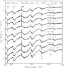 |
Fig. 2 Same as Fig. 1, but for SpTs between M3 and M5. |
| In the text | |
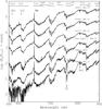 |
Fig. 3 Same as Fig. 1, but for SpTs later than M5. |
| In the text | |
|
Fig. 4 Distribution of spectral types of the Class III YSOs discussed in this work. Each bin corresponds to one spectral subclass. |
| In the text | |
|
Fig. 5 Example of the combination of a flux-calibrated and telluric removed X-shooter spectrum (black) with model spectra with the same Teff (green), which is normalized at the red and blue edges of the X-shooter spectrum and only shown outside the X-shooter range. The telluric bands in the NIR are replaced with a linear interpolation (red). In this figure we show the example of TWA14. |
| In the text | |
|
Fig. 6 Hertzsprung-Russell Diagram of the Class III YSOs of this work. Data points are compared with the evolutionary tracks (dotted lines) by Baraffe et al. (1998). Isochrones (solid lines) correspond to 2, 10, 30, and 100 Myr. |
| In the text | |
|
Fig. 7 Portion of the spectrum, showing emission in all Balmer lines from Hβ up to H12, as well as the CaII H and K lines, of the YSO TWA13B. The spectrum has been smoothed to a resolution R = 3750 at 375 nm. |
| In the text | |
|
Fig. 8 Hα equivalent width as a function of spectral type. The dashed lines represent the boundary between accretors and nonaccretors proposed by White & Basri (2003) for different SpT. |
| In the text | |
|
Fig. 9 Hα equivalent width as a function of the 10% Hα width. The vertical dashed line rerpesents the White & Basri (2003) criterion for the boundary between accretors and nonaccretors. The objects with 10% Hα width bigger than 270 km s-1 are, from right to left: Sz122, Sz121, TWA6, and TWA13A. |
| In the text | |
|
Fig. 10 log (Lacc,noise/L⊙) obtained using different accretion tracers and the relations between Lline and Lacc from Alcalá et al. (in prep.). The mean values obtained using the Balmer and HeIλ587.6 lines are shown with the blue solid lines, and the 1σ dispersion is reported with the blue dashed lines. Upper limits are reported with red empty triangles. The 10% Hα width is reported with a blue filled circle. |
| In the text | |
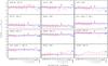 |
Fig. 11 Same as Fig. 10. |
| In the text | |
|
Fig. 12 Mean values of log (Lacc,noise/L⊙) obtained with different accretion diagnostics as a function of Teff. Error bars represent the standard deviation around the mean log (Lacc,noise/L⊙). These data should be intended as the noise in the values of Lacc due to chromospheric emission flux. |
| In the text | |
|
Fig. 13 Mean values of log (Lacc,noise/L∗) obtained with different accretion diagnostics as a function of log Teff. The dashed line is the best fit to the data, whose analytical form is reported in Eq. (2). Two objects (Sz122 and TWA9A) are excluded from the fit (empty symbols), as explained in the text. |
| In the text | |
|
Fig. 14 log Ṁacc,noise as a function of log M∗, with values of Ṁacc,noise obtained using three different isochrones from Baraffe et al. (1998) and the values of Lacc,noise/L∗ derived from the fit in Eq. (2) at any Teff. Results using the 1 Myr isochrone are reported with filled circles, those using the 3 Myr isochrone with filled triangles, and those using the 10 Myr isochrone with filled squares. |
| In the text | |
|
Fig. 15 log Ṁacc as a function of log M∗ for Class II objects located in different star forming regions. Data for ρ Oph are from Natta et al. (2006), corrected for new distance measurements by Rigliaco et al. (2011); ONC points are from Manara et al. (2012), data for L1630N and L1641 are from Fang et al. (2009), and those for ChaII from Biazzo et al. (2012). Ṁacc values obtained with indirect methods are shown with colored, filled points, while measurements based on the direct U-band excess method are shown with gray empty points as a reference. Downwards triangles refer to upper limits. The thick red solid line is the lower limit to the measurements of Ṁacc set by chromospheric activity in the line emission. We use the values for the correct isochrone according to the mean value of the age for each region, as reported on the plot. |
| In the text | |
|
Fig. B.1 Spectral type of the objects as a function of the spectral index values obtained with different NIR indices (Table B.1). Red symbols are values from this work, while green crosses are from Testi et al. (2001) and Testi (2009). Red stars are used for objects with SpT in the range of validity of the index, while red pentagons for those not in the range of validity of the index. Dashed lines are the best fit from the reference cited in Table B.1 for each index, when available. No published relations are available for the indices IJ and IK. Black and red solid lines are the best fits (black = linear, red = polynomial) from this work, considering both our sample and the values from the literature. |
| In the text | |
|
Fig. C.1 Spectra of Class III YSOs with spectral type earlier than M3 in the NIR arm. All the spectra are normalized at 1700 nm and offset in the vertical direction by 0.5 for clarity. The spectra are also smoothed to the resolution of 2000 at 2000 nm to make identification of features easier. |
| In the text | |
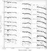 |
Fig. C.2 Same as Fig. C.1, but for spectral types between M3 and M5. |
| In the text | |
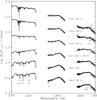 |
Fig. C.3 Same as Fig. C.1, but for spectral types later than M5. |
| In the text | |
|
Fig. C.4 Spectra of Class III YSOs with spectral type earlier than M2 in the UVB arm. All the spectra are normalized at 450 nm and offset in the vertical direction for clarity. The spectra are also smoothed to the resolution of 1500 at 400 nm to make identification of features easier. |
| In the text | |
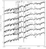 |
Fig. C.5 Same as Fig. C.4, but for spectral types between M2 and M4. |
| In the text | |
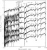 |
Fig. C.6 Same as Fig. C.4, but for spectral types later than M4. |
| In the text | |
Current usage metrics show cumulative count of Article Views (full-text article views including HTML views, PDF and ePub downloads, according to the available data) and Abstracts Views on Vision4Press platform.
Data correspond to usage on the plateform after 2015. The current usage metrics is available 48-96 hours after online publication and is updated daily on week days.
Initial download of the metrics may take a while.