| Issue |
A&A
Volume 551, March 2013
|
|
|---|---|---|
| Article Number | A142 | |
| Number of page(s) | 11 | |
| Section | Catalogs and data | |
| DOI | https://doi.org/10.1051/0004-6361/201220863 | |
| Published online | 11 March 2013 | |
The seven year Swift-XRT point source catalog (1SWXRT)⋆
1 ASI – Science Data Center, via Galileo Galilei, 00044 Frascati, Italy
e-mail: This email address is being protected from spambots. You need JavaScript enabled to view it.
2 INAF – Osservatorio Astronomico di Roma, via Frascati 33, 00040 Monteporzio Catone, Italy
3 Department of Astronomy and Astrophysics, Pennsylvania State University, University Park, Pennsylvania 16802, USA
4 INAF – Osservatorio Astronomico di Brera, via E. Bianchi 46, 23807 Merate (LC), Italy
5 INAF – Istituto di Astrofisica Spaziale e Fisica Cosmica di Palermo, via U. La Malfa 153, 90146 Palermo, Italy
6 Dept. of Physics and Astronomy, University of Leicester, Leicester, LE1 7RH, UK
7 NASA – Goddard Space Flight Center, Greenbelt, 20771 Maryland, USA
Received: 6 December 2012
Accepted: 28 December 2012
Abstract
Context. The Swift satellite is a multi-wavelength observatory specifically designed for gamma-ray burst (GRB) astronomy that is operational since 2004. Swift is also a very flexible multi-purpose facility that supports a wide range of scientific fields such as active galactic nuclei, supernovae, cataclysmic variables, Galactic transients, active stars and comets. The Swift X-ray Telescope (XRT) has collected more than 150 Ms of observations in its first seven years of operations.
Aims. The purpose of this work is to present to the scientific community the list of all the X-ray point sources detected in XRT imaging data taken in photon counting mode during the first seven years of Swift operations. All these point-like sources, excluding the GRB, will be stored in a catalog publicly available (1SWXRT).
Methods. We considered all the XRT observations with exposure time longer than 500 s taken in the period 2005−2011. Data were reduced and analyzed with standard techniques and a list of detected sources for each observation was produced. A careful visual inspection was performed to remove extended, spurious and piled-up sources. Finally, positions, count rates, fluxes, and the corresponding uncertainties were computed.
Results. We have analyzed more than 35 000 XRT fields, with exposures ranging between 500 s and 100 ks, for a total exposure time of almost 140 Ms. The catalog includes approximately 89 000 entries, of which almost 85 000 are not affected by pile-up and are not GRBs. Considering that many XRT fields were observed several times, we have a total of ~36 000 distinct celestial sources. We computed count rates in three energy bands: 0.3−10 keV (Full, or F), 0.3−3 keV (Soft, or S) and 2−10 keV (Hard, or H). Each entry has a detection in at least one of these bands. In particular, we detect ~80 000, ~70 000 and ~25 500 in the F, S and H band, respectively. Count rates were converted into fluxes in the 0.5−10, 0.5−2 and 2−10 keV bands. The flux interval sampled by the detected sources is 7.4 × 10⁻¹⁵ − 9.1 × 10⁻¹¹, 3.1 × 10⁻¹⁵ − 1.1 × 10⁻¹¹ and 1.3 × 10⁻¹⁴ − 9.1 × 10⁻¹¹ erg cm-2 s-1 for the F, S and H band, respectively. Some possible scientific uses of the catalog are also highlighted.
Key words: catalogs / surveys / X-rays: general
Catalog is only available at the CDS via anonymous ftp to cdsarc.u-strasbg.fr (130.79.128.5) or via http://cdsarc.u-strasbg.fr/viz-bin/qcat?J/A+A/551/A142
© ESO, 2013
1. Introduction
The Swift gamma-ray burst Explorer (Gehrels et al. 2004) is a NASA mission, successfully launched on 2004 Nov. 20. The hardware and software were built by an international team involving US, United Kingdom and Italy, with contributions from Germany and Japan. The main scientific driver of the Swift mission is to detect gamma-ray bursts (GRBs) in the hard X-ray band with the Burst Alert Telescope (BAT, Barthelmy et al. 2005) and quickly follow-up their emission at longer wavelength with the X-Ray Telescope (XRT, Burrows et al. 2005) and Ultraviolet/Optical Telescope (UVOT, Roming et al. 2005).
Despite being specifically designed to address GRB science topics, Swift is also an effective multi-purpose multi-frequency observatory. The Swift team expertise in following up GRBs has grown during the satellite operations, leading to an evolution of the observing time share between GRBs and other cosmic sources. At the beginning of the satellite operations (up to 2006, Romano 2012), approximately 56% of the Swift observing time was dedicated to GRB observations, and ~26% divided up between target of opportunity (ToO, ~ 8%) and “fill-in” observations (that are short exposures of a variety of X-ray sources taken when Swift was not engaged in GRB science, ~18%). After 2006, it became evident that there was no need to follow up all GRBs for a very long time. Thus, without losing too much relevant scientific information, in 2010 the GRB dedicated time dropped to ~27% while ~29% and ~26% was allocated to ToO and Fill-in observations, respectively. In the remaining ~18% of the time the satellite flies through the South Atlantic Anomaly or is devoted to calibration issues.
The Swift mission is currently producing data at a pace of about ~500 observations per month, contributing to most areas of astronomy. Apart from GRBs, the Swift instruments are observing extragalactic targets, such as active galactic nuclei (AGNs), clusters of galaxies, nearby galaxies, and Galactic sources, such as binaries, microquasars, pulsars, and all Galactic variable sources in general.
The Swift-XRT utilizes a mirror set built for JET-X and an XMM/EPIC MOS CCD detector to provide a sensitive broad-band (0.2−10 keV) X-ray imager with effective area of >120 cm2 at 1.5 keV, field of view of 23.6 × 23.6 arcmin, and angular resolution of 18 arcsec. The detection sensitivity is 2 × 10-14 erg cm-2 s-1 in 104 s. The instrument can work in three different modes (Hill et al. 2004): photodiode (PD), windowed-timing (WT) and photon-counting (PC) modes. Due to a micrometeorite hit on May 27 2005, the PD mode has been disabled because of the very high background rate from hot pixels which cannot be avoided during read-out in this mode (Abbey et al. 2006). While the first two modes are built to produce a high time resolution at the expense of losing all (PD) or part (WT) of the spatial information, the latter one retains full imaging resolution and will be the only mode exploited here.
This paper presents the 1SWXRT catalog, which consists of all the point-like sources detected by the XRT in its first seven years of operations (2005−2011). Updated versions of the catalog, containing observations performed from 2012, are foreseen on timescales of about two years. Similar catalogs have already been produced for the first eight years of Chandra operations (Evans et al. 2010) and for the first seven years of XMM-Newton operations (Watson et al. 2009). The reduction and analysis method is very similar to that adopted for the production of the “Swift Serendipitous Survey in deep XRT GRB fields” (Puccetti et al. 2011), which comprises a list of sources detected in all Swift-XRT GRB fields with exposure times larger than 10 ks, observed by Swift between 2004 and 2008. Our goal is complementary to that of Puccetti et al. (2011). Instead of summing all the observations related to the same field, we keep them separated, in order to build a catalog which retains information about the variability of our sources. In addition, we analyzed all the XRT observations, and not only the fields centered on GRBs. A future work (Evans et al., in prep.) will consider all XRT fields, combined where the same field is observed multiple times. A first catalog of extended sources has been published (Tundo et al. 2012), and further updates are in preparation. Our paper is organized as follows. In Sect. 2 we briefly describe our catalog. In Sects. 3 and 4 we present the data reduction and analysis method, respectively. In Sect. 5 we briefly discuss the scientific issues that can be tackled using our catalog. Finally, in Sect. 6 we draw our conclusions.
2. The seven year Swift-XRT point source catalog
The seven year Swift-XRT point source catalog (1SWXRT) is built using all the observations performed by Swift-XRT in PC observing mode between 2005 and 2011. We consider in our analysis all the XRT fields, including “safe pointings”, that are sky positions used by the satellite as safe positions in case there are troubles during the slew from one target to another. The only constraint for a field to be analyzed is on the exposure time, which is required to be larger than 500 s. Different observations are not merged, but analyzed separately, thus retaining information about the variability of the cataloged sources. Here and in the following we define as “observation” the total exposure time per target for a given day, identified by an unambiguous sequence number.
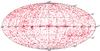 |
Fig. 1 Aitoff projection in Galactic coordinates of the Swift-XRT fields analyzed in this paper. |
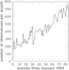 |
Fig. 2 Number of Swift-XRT observations with exposure time longer than 500 s acquired every month from January 1st 2005. |
The total number of observations considered is 35 011, for an overall exposure time of ~140 Ms. Figure 1 shows the Aitoff projection in Galactic coordinates of these XRT observations. Table 1 collects the number of observations per month in the period 2005−2011, together with the corresponding exposure time. Figure 2 shows the number of observations as a function of the month in which they were performed. It is interesting to note how this number increased with time, reflecting the evolution of the Swift observing policy. Figure 3 displays the number of observations grouped in bins of exposure time (500 s binning). Most of the observations have short exposures. In fact, ~18% have texp < 1 ks and ~77% have texp < 5 ks. Only 7% of the observations have an exposure time >10 ks, which are mostly (but not exclusively) fields associated with GRBs. A bump at about 10 ks is evident in Fig. 3. This happens because GRBs are typically observed for 10 ks per day, so that a lot of observations have that exposure duration.
Many of the ~35 000 fields analyzed are repeated pointings centered on the same sky position. To estimate the total sky coverage of our data set, when fields were observed more than once, we considered only the deepest exposure. This leaves us with 8644 distinct fields, whose geometrical sky coverage as a function of the exposure time is plotted in Fig. 4. The cumulative sky coverage of all our distinct fields, which by definition have exposure times texp > 500 s is 1300 square degrees. A full list of the observations analyzed in this work is available online1.
In the next sections we will discuss how these raw observations have been reduced and analyzed, to detect and gather information on the sources that make up the XRT catalog.
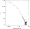 |
Fig. 3 Exposure time distribution for the XRT sources analyzed in this work. The time bin is 500 s. |
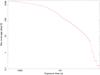 |
Fig. 4 Sky coverage of the Swift-XRT fields as a function of the exposure time (cumulative distribution). |
3. XRT data reduction
The XRT data were processed using the XRTDAS software (v. 2.7.0, Capalbi et al. 2005) developed at the ASI Science Data Centre and included in the HEAsoft package (v. 6.11) distributed by HEASARC. For each observation of the sample, calibrated and cleaned PC mode event files were produced with the xrtpipeline task. In addition to the screening criteria used by the standard pipeline processing, we applied two further, more restrictive screening criteria to the data, in order to improve the signal to noise ratio (S/N) of the faintest, background dominated, serendipitous sources.
First, we selected only time intervals with CCD temperature less than − 50 °C (instead of the standard limit of − 47 °C) since the contamination by dark current and hot pixels, which increase the low energy background, is strongly temperature dependent. Second, background spikes can occur in some cases, when the angle between the pointing direction of the satellite and the bright Earth limb is low. To eliminate this so-called bright Earth effect, due to the scattered optical light that usually occurs toward the beginning or the end of each orbit, we monitored the count rate in four regions of 70 × 350 physical pixels, located along the four sides of the CCD. Then, through the xselect package, we excluded time intervals when the count rate is greater than 40 counts/s. This is enough to remove the bright Earth contamination from most (but not all, see next section) of the XRT observations.
We produced exposure maps of the individual observations, using the task xrtexpomap. Exposure maps were produced at three energies: 1.0 keV, 4.5 keV, and 1.5 keV. These correspond to the mean values for a power-law spectrum of photon index Γ = 1.8 (see Sect. 4.3) weighted by the XRT efficiency over the three energy ranges considered here: 0.3−3 keV (soft band S), 2−10 keV (hard band H), 0.3−10 keV (full band F). For each observation we also produced a background map, using XIMAGE, by eliminating the detected sources and calculating the mean background in box cells of size 32 × 32 pixels.
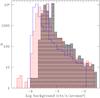 |
Fig. 5 Distribution of the mean background counts/sec/arcmin2 for our XRT observations, in the F band (black-shaded histogram), S band (red-shaded histogram) and H band (blue histogram). |
Figure 5 shows the distribution of the mean background counts/s/arcmin2 in the F, S and H energy bands. The median values of background and their interquartile ranges are  counts/ks/arcmin2,
  counts/ks/arcmin2 and
  counts/ks/arcmin2 for the F, S and H band, respectively. These median values correspond to a level of 1.1, 0.77 and 0.47 counts in the F, S, and H band, respectively, over a typical source detection cell (see Sect. 4) and an exposure of 100 ks, which is the highest exposure time for all our observations.
4. Data analysis
4.1. Detection and filtering procedure
The point source catalog was produced by running the detection algorithm detect, a tool of the XIMAGE package version 4.4.12. Detect locates the point sources using a sliding-cell method. The average background intensity is estimated in several small square boxes uniformly located within the image. The position and intensity of each detected source are calculated in a box whose size maximizes the S/N. The net counts are corrected for dead times and vignetting using the input exposure maps, and for the fraction of source counts that fall outside the box where the net counts are estimated, using the point-spread function (PSF) calibration. Count rate statistical and systematic uncertainties are added quadratically. Detect was set to work in bright mode, which is recommended for crowded fields and fields containing bright sources, since it can reconstruct the centroids of very nearby sources (see the XIMAGE help). While producing the deep Swift-XRT catalog, Puccetti et al. (2011) found that background is well evaluated for all exposure times using a box size of 32 × 32 original detector pixels, and that the optimized size of the search cell that minimizes source confusion, is 4 × 4 original detector pixels. The background adopted by XIMAGE for each observation is an average of the background evaluated in all the 32 × 32 individual cells. We adopted these cell sizes and background estimation method too, and we also set the signal-to-noise acceptance threshold to 2.5. We produced a catalog using a corresponding Poisson probability threshold of 4 × 10⁻⁴. We applied detect on the XRT image using the original pixel size, and in the three energy bands: F, S and H (see Sect. 3).
The catalog was cleaned from spurious and extended sources by visual inspection of all the observations. Spurious sources arise on the the wings of the PSF of extremely bright sources, or near the edges of the XRT CCD (where the exposure map drastically drops out), or as fluctuations on extended sources and in some cases as residual bright Earth contamination not completely eliminated by our screening criteria. To deal with this last source of spurious detections, we run the detect algorithm on the observations affected by bright Earth, lowering the count rate threshold value on the corners of the detector, as defined in Sect. 3. In a few cases, to avoid lowering the threshold excessively, and thus exclude too many time intervals from the analysis, we decided to manually remove the spurious sources associated with residual bright Earth contamination even after the adopted cleaning criteria described in Sect. 3. About 200 observations out of the entire sample of ~35 000 (~0.6%) needed a manual removal of spurious sources induced by bright Earth background. Extended sources have also been eliminated from the final point-like catalog, because detect is not optimized to detect this type of sources, not being calibrated to correct for the background and PSF loss in case of extended sources. To clean the catalog from extended sources, we compare their brightness profile with the XRT PSF at the source position on the detector, using XIMAGE. In total, ~3700 observations needed a manual removal of spurious and/or extended sources, which is ~10% of the total fields analyzed.
4.2. Source statistics
The above procedure resulted in 89 053 point-like objects detected in at least one of the three bands. Of these, 1947 are affected by pile-up, i.e., feature more than 0.6 counts in the full band, while 2166 are GRBs, which will not appear in this catalog. After removing GRBs and piled-up sources, we are left with 84 992 entries, which define a “good” sample.
As explained before, not all these detections represent distinct sources, since observations of some fields are repeated many times. To obtain an estimate of the number of independent celestial sources, we compress our catalog over a radius of 12 arcsec. In other words, all entries within 12 arcsec of each other are counted once. The choice of the compressing radius is not straightforward. In fact, too large a radius would lead to the compression of sources that are really different, while too small a value would result in counting the same source more than once, as it could have a slightly different position in different observations due to statistical and systematic uncertainties. We tried different compressing radii, and we noted that the number of compressed sources increases slightly while reducing the radius up to 12 arcsec, while this increment is huge with a further reduction of the compressing parameter. This means that below 12 arcsec we are beginning to count the same sources more than once. This number is close to twice the typical uncertainty of the weakest sources in the XRT fields, which is roughly of 6−7 arcsec. The estimated number of independent celestial sources obtained in this way is ~36 000. In this section, however, we will consider every one of the 84 992 entries of the catalog, because of the observation-by-observation analysis we decided to perform to build our database.
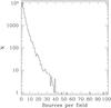 |
Fig. 6 Distribution of the detected sources per field. Each source in this plot is detected in at least one of the three bands. Fields with more than 40 sources have high exposure times. |
Number of sources detected in each band and any combination of them.
Table 2 shows the detections in each of the three bands and in all possible combinations of them. In particular, 80 123 sources are detected in the F band, 70 018, in the S band and 25 437 in the H band. Figure 6 plots the histogram of the number of sources detected per field. Most of the observations present few sources, with ~ 51% of the fields having just one or no detections and less than 5% showing more than 10 sources. This is a consequence of the features of our sample, composed by many observations with a low exposure time.
4.3. Count rates and fluxes
As explained in Sect. 4.1, the count rates are estimated through the detect algorithm in the F, S, H bands and corrected using proper exposure maps (i.e., taking bad columns and vignetting into account) and PSF. To assess the reliability of the count rates evaluated with detect, Puccetti et al. (2011) selected a sample of 20 sources at different off-axis angles, and compared the detect results with that obtained by extracting the source spectra in a region of 20 arcsec. The average ratio between the count rates estimated using the two methods resulted to be 1.1 ± 0.2, confirming the reliability of our method. Figure 7 shows the distribution of the count rates in the three energy bands. The median values of the count rates are 3.86 × 10⁻³, 3.85 × 10⁻³ and 6.89 × 10⁻³ cts s-1 in the F, S and H band, respectively. The faintest objects have been detected in the longest exposure time observations. The lowest count rate values estimated are ~2.1 × 10⁻⁴, ~1.8 × 10⁻⁴ and ~1.5 × 10⁻⁴ cts s-1 in the F, S and H band, respectively.
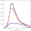 |
Fig. 7 Distribution of the count rates in the full (black), soft (red) and hard (blue) bands. |
Count rates in the F, S and H bands were converted to 0.5−10, 0.5−2 and 2−10 keV observed fluxes, respectively. We adopted these flux bands to be consistent with previously published works (e.g., Watson et al. 2009; Evans et al. 2010). The conversion was made under the assumption that the spectral shape of each source is described by an absorbed power-law. The hydrogen column density (NH) in the direction of our target is assumed to be the Galactic one, while the photon spectral index Γ has been estimated through the hardness ratio3. The latter quantity is defined, for each source, as HR = (cH − cS)/(cH + cS), cS and cH being the count rates in the S and H band, respectively. Figure 8 plots the hardness ratio distribution of our sources and their spectral indices. The median value of the hardness ratio is HRM = −0.38, while the distribution peaks at HRP = −0.50. However, HR can be evaluated only for objects with a detection in both the S and H bands, which are 21 097 out of a total of 84 992, i.e., ~25% of our sample (see Table 2). For sources which miss the detection in one of these two bands, the Γ slope must be chosen somehow. One way would be to compute the average or the median of all the Γ values of our sources. However, this is not the best strategy, because Γ strongly depends on the source type, and our sample is highly heterogeneous. Thus, we decide to fix the photon index of the sources with a missing S or H count rate to Γ ≡ 1.8, following Puccetti et al. (2011). In fact, they computed the most probable hardness ratio value (HR = −0.5) in a subsample of their catalog comprizing all the high Galactic-latitude (|b| > 20deg) sources. This HR value, combined with the median of the Galactic hydrogen column density (NH = 3.3 × 1020 cm-2, Kalberla et al. 2005), corresponds to Γ = 1.8. This choice should provide a reliable flux estimate for our extragalactic sources, which constitute most of our catalog. However, the reader must be aware that the flux computed this way may represent just a rough estimate for other type of sources (see also next sub-section for a more detailed description about the flux uncertainties). The faintest fluxes sampled by our survey belong to the sources detected in the deepest observations. In detail, we find that the flux interval sampled by the detected sources is in the range 7.4 × 10⁻¹⁵−9.1 × 10⁻¹¹, 3.1 × 10⁻¹⁵−1.1 × 10⁻¹¹ and 1.3 × 10⁻¹⁴−9.1 × 10⁻¹¹ erg cm-2 s-1 for the F, S and H band, respectively.
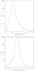 |
Fig. 8 Top panel: hardness ratio distribution of our sample. Bottom panel: distribution of the X-ray spectral indices for our sample. These plots include only sources with a detection in both the S and H bands. |
We provide 90% count rate and flux upper limits every time a source is not detected in one or two of the considered bands. The 90% count upper limit for a given background is defined as the number of counts necessary to be interpreted as a background fluctuation with a probability of 10% or less, according to a Poissonian distribution. In other words, if the background of our field is B, we are searching the upper limit X for which  (1)where M is the number of counts measured at the position of each source in a region of 16.5 arcsec radius, which corresponds to a fraction of the PSF of ~68%. Equation (1) does not take into account possible background fluctuations that may arise close to the considered source. The correction factor has been evaluated by Puccetti et al. (2011) following the recipe in Bevington & Robinson (1992). They found that the factor 1.282 × σ (with
  describing the Poissonian background fluctuations) must be added to the count upper limits. The count rate upper limits are finally evaluated from these counts (which are corrected for the non-included PSF fraction of the cell), by dividing them for the net exposure, which takes the vignetting at the source position into account. Flux upper limits are computed from count rate upper limits, adopting the appropriate NH and assuming Γ = 1.8, as explained before.
Source parameters in the catalog.
1SWXRT catalog template.
4.4. Uncertainties and source reliability
Detect count rates are associated with their statistical (Poissonian) uncertainties. These errors are propagated to the flux estimates, but here the main uncertainty is the variety of the spectral behavior of different sources. To determine the flux variation with the spectral parameters, we estimate the count rate-to-flux conversion factors for a wide range of spectral slopes (Γ = 0−2) and hydrogen column densities (NH = 1019 − 1022 cm-2). The conversion factors are in the range (2.9−15) × 10-11, (0.9−1.5) × 10-11 and (8.1−17) × 10-11 erg cm-2 s-1 for the F, S and H band, respectively. The conversion factor for the F band is more sensitive to the spectral shape than for the S and H bands, because this band is wider.
Concerning the source positions, their errors are both statistical and systematic, with the total positional uncertainty being:  (2)The systematic error σsys is due to the uncertainty on the XRT aspect solution. This quantity has been estimated by Puccetti et al. (2011) by cross-correlating a sub-sample of bright sources of their XRT-deep catalog with the SDSS optical galaxy catalog. They found that the mean σsys at the 68% confidence level is 2.05 arcsec, a value consistent with previous results by Moretti et al. (2006). This value represents the number we will adopt in estimating the positional error in Eq. (2). The statistical variance
  is instead inversely proportional to the source number counts.
To assess the reliability of our detections we must address the possibility of source confusion. The source confusion issue arises when two close sources are detected as a single one. This problem may be important if the distances between two objects is of the order of the cell detection of the algorithm detect. To evaluate the possibility of source confusion, we compute the probability of finding two sources with a X-ray flux higher than a certain threshold Flim, lying at a distance smaller than θmin:  (3)Here we adopt as θmin twice the typical size of the cell detection box (4 pixels or 9.44 arcsec), while N is the number counts corresponding to Flim, which can be evaluated, e.g., from the C-COSMOS survey (Elvis et al. 2009). Our deepest field has an exposure of ~100 ks. Using the Flim corresponding to the count rates of the faintest sources detected in this field (~1.7 × 10⁻⁴ and ~1.5 × 10⁻⁴ cts/s in the S and H band, respectively), we find that the source confusion probability is less than 3% in both the S and H band. This is of course the field in which the source confusion probability is highest. For fields of ~10 ks (~93% of our sample has exposures <10 ks) the flux limits are shallower by a factor of ~3. Applying Eq. (3) to these fields results in a probability of source confusion of ~0.9% and ~0.3% in the S and H band, respectively. This means that source confusion is negligible in our sample.
4.5. 1SWXRT description
The final catalog comprises 32 field parameters for each entry. Source name, position, count rates and fluxes, exposure, hardness ratio and galactic NH are reported, together with the corresponding uncertainties and/or reliabilities. A full description of all the parameters is presented in Table 3. Table 4 gives instead the first ten entries of the catalog as an example.
5. Scientific use of the catalog
A full exploitation of the scientific data presented in this work is far beyond the scope of the present paper. Nevertheless, we would like to draw the reader’s attention to some of the scientific topics that can be addressed using 1SWXRT.
5.1. Short-term variability
As stated in the previous section, in our analysis we do not merge observations pointing to the same field, so we can study the variability of sources observed more than once. Since many observations are often performed consecutively, this enables to determine short-term variability for the involved sources.
Our database comprises 12 908 sources observed at least twice. Among these, we select all sources detected in each observation in the soft or hard band. 7936 and 2113 sources are detected in the soft and hard band, respectively. Figure 9 plots the distribution of the number of sources observed many times, while Fig. 10 displays the histogram for the variability as a function of the σ significance. The number of sources in the soft band with a variation larger than 3σ and 5σ is 1774 and 623, respectively, i.e., a fraction of 22% and 7.7% of the total soft sources. Similarly, the number of sources in the hard band with a variation larger than 3σ and 5σ is 447 and 148, respectively, i.e., a fraction of 21% and 7.6% of the total hard sources. Thus, variability is observed in both bands, and with similar trends. However, some tens of sources show extreme variability (Fig. 10). The ratio of such extreme variable sources with respect to the total number grows stronger in the hard band with respect to the soft one as the significance of the variability increases. For example, the fraction of sources which vary at more than 10σ is 1.7% and 1.9% in the soft and hard band, respectively, while at the 20σ level, the fractions become 0.4% (soft) and 0.7% (hard).
We then select all the sources observed at least 5 times. Figure 11 shows the cumulative distribution of the statistical significance of the variability for sources with five observations or more. This variability significance has been computed with respect both to the maximum and to the minimum fluxes. It interesting to note that the variability is more pronounced when considering the maximum fluxes. In other words, the average fluxes are in general closer to the minimum values than to the maximum ones. This could be a possible indication that we are observing short-duration flares in some sources, with the normal state being close to the minimum value observed.
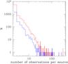 |
Fig. 9 Distribution of the number of sources observed more than once. Red line refers to the soft band, blue line to the hard one. |
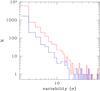 |
Fig. 10 Distribution of the source variability expressed as a function of the σ significance. Red line refers to the soft band, blue line to the hard one. |
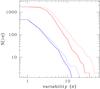 |
Fig. 11 Cumulative distribution of the statistical significance of the variability for sources with five observations or more. Red (blue) lines refer to the soft (hard) band. Solid (dotted) lines refer to the variability significance of the minimum (maximum) flux values with respect to the average ones. |
5.2. Soft sources
We can use our dataset to study sources showing emission in the soft band only. Among these, one important class is represented by isolated neutron stars (INS, see, e.g., Treves et al. 2000; Haberl et al. 2003; Haberl 2004).
INS are blank field sources, i.e., X-ray sources with no or very faint counterparts in other wavelength domains. Concerning the X-ray-to-optical flux ratio, values of fX/fopt > 103 define the INS class, but in some cases values as high as 105 have been reported. The X-ray emission is supposed to be produced by some residual internal energy (coolers) or because they are interacting with the interstellar medium (accretors). The INS X-ray spectrum is well fitted by a soft blackbody, with temperatures of ~100 eV. This means that basically no X-ray emission above ~2 keV is expected. Given the low column densities measured for these objects, the emission is consistent with being produced from the neutron star surface (see, e.g., Walter & Lattimer 2002). Other characteristics often exhibited by these sources (coolers) are a periodicity of ~5−10 s, absorption features below 1 keV and closeness. These elusive sources are of extreme importance, because they could represent ~1% of the total number of stars in our Galaxy. To pinpoint their properties means to understand the end-point of the evolution of a large class of stars. To date, only 8−10 objects of this class have been identified.
To check our catalog for the presence of INS, and in general to categorize the soft objects, we selected all sources that do not show emission in the full and hard band. When considering objects observed more than once, we excluded from our analysis all sources in which there is a detection in the full or hard band in at least one observation. This helps us to include in our sample just genuine soft emitters, and to exclude part of the sources that are possibly not detected in the hard band due to low exposure times.
We selected 2087 objects following the above criteria. Figure 12 displays the 0.5−2 keV flux distribution for these sources. The histogram bin size is set to 0.05 dex. Since the soft band is in general more sensitive than the hard one, the faint part of this distribution can still comprise normal sources that are not detected in the 2 − 10 keV range due to a flux level below the sensitivity threshold. However, we determined the number of XRT sources featuring at least 50 or 100 counts in the 0.5−2 keV band, without detection in the 2−10 one. We obtain 7 sources with at least 50 counts. Of these, 3 have more than 100 counts. These seven objects are good INS candidates.
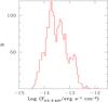 |
Fig. 12 Distribution of the 0.5−2 keV flux for the sources detected in the soft band only. |
5.3. Hard sources
In a similar way to what described in the previous sub-section, we can search our dataset for sources which show emission in the hard band only. To categorize the hard objects, we selected all sources that do not show emission in the full and soft band. When considering objects observed more than once, we excluded from our analysis all sources in which there is a detection in the full or soft band in at least one observation. This helps us to include in our sample just genuine hard emitters, and to exclude part of the sources that are possibly not detected in the soft band due to a low exposure time coupled with an unusual background level. 308 objects in our dataset fulfill the above criteria. Figure 13 displays the 2−10 keV flux distribution for these sources. The histogram bin dimension is set to 0.1 dex. The hard band is less sensitive than the soft one. Thus, contrary to the case of the soft sources, we are confident that this sub-sample contains genuine hard sources only.
The main type of objects contributing to this sub-sample are expected to be obscured AGNs, whose discovery and study is very important both to study the properties and evolution of the accretion process onto supermassive black holes residing at the center of galaxies and to determine their contribution to the X-ray background, in particular to its peak emission in the 20−30 keV band that still remains largely unexplained (see, e.g., Gilli et al. 2007; Treister et al. 2009, and references therein). In future works we will investigate on the nature of these sources in order to determine their properties and nature.
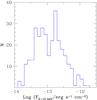 |
Fig. 13 Distribution of the 2−10 keV flux for the sources detected in the hard band only. |
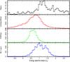 |
Fig. 14 Distribution of the X-ray spectral index for specific source types in our catalog. |
5.4. Cross-correlation with multi-wavelength catalogs
Our catalog can be cross-correlated with multi-wavelength ones, to obtain statistical information about specific class of sources. Here, we cross-correlated the XRT catalog with BZCAT, a multifrequency catalog of blazars (Massaro et al. 2009). We stress that this is just an example, and that many more cross-correlations with other catalogs can be performed to fully exploit 1SWXRT.
Blazars are radio loud AGN pointing their jets in the direction of the observer (see e.g. Urry & Padovani 1995). They come in two main subclasses, the flat spectrum radio quasars (FSRQs), which show strong, broad emission lines in their optical spectrum, just like radio quiet QSOs, and BL Lacs, which are instead characterized by an optical spectrum, which at most shows weak emission lines or is completely featureless. The strong non-thermal radiation is composed of two basic parts forming two broad humps in the ν vs. νFν plane, the low-energy one attributed to synchrotron radiation, and the high-energy one, usually thought to be due to inverse Compton radiation (Abdo et al. 2010). The peak of the synchrotron hump ( ) can occur at different frequencies. In FSRQs never reaches very high values ( ≲ 1014.5 Hz), whereas the of BL Lacs can reach values as high as ≳ 1018 Hz (e.g. Giommi et al. 2012).
The cross-correlation between the BZCAT and 1SWXRT catalogs has been performed by matching the coordinates over an error radius of 0.2 arcmins. We found 938 sources in 1SWXRT with a BZCAT counterpart. Of these, 524 are FSRQs and 414 are BL Lacs. Figure 14 shows the X-ray spectral index distribution for these sources. It is evident that BL Lac distribution is softer than FSRQ one. This is because the X-ray 0.5−10 keV band samples on average the high energy tail of the synchrotron emission in BL Lacs, where νFν is decreasing. On the other hand, the same energy band describes, on average, the low energy tail of the inverse Compton emission in FSRQs, where νFν is instead increasing. For comparison, Fig. 14 plots also the X-ray spectral index of the stars, obtained by cross-correlating the XRT catalog with the Smithsonian Astrophysical Observatory Star Catalog (SAO), and that of the unidentified sources.
6. Summary and conclusions
We have reduced and analyzed all the observations performed by Swift-XRT in PC mode with an exposure time longer than 500 s, during its first seven years of operations, i.e., between 2005 and 2011. Approximately 35 000 XRT fields have been analyzed, with net exposures (after screening and filtering criteria being applied) ranging from 500 s to 100 ks. The total, net exposure time is ~140 Ms.
The purpose of this work was to create a catalog (1SWXRT) of all the point like sources detected in these observations. To this purpose, we run the XIMAGE detect algorithm to all our fields, and then removed spurious and extended sources through visual inspection of the XRT observations. The total number of point-like objects detected is 89 053, of which 2166 are GRB detections (so transient sources by definition) and 1947 are sources affected by pile-up. Thus, our final version of the catalog comprises 84 992 entries, which define the “good” sample. Many entries represent the same sources, since several portions of the sky have been observed many times by XRT. To estimate an approximate number of distinct, celestial sources, we compress our catalog over a radius of 12 arcsec, a typical positional uncertainty value in faint XRT sources. In other words, all entries closer than 12 arcsec are counted once, and the result of this procedure is ~36 000 distinct sources.
For all the entries of 1SWXRT, we determined the position, the detection probability and the S/N. Count rates were estimated in the 0.3−10, 0.3−3 and 2−10 keV bands. Each source has a detection in at least one of these bands, with ~80 000, ~70 000 and ~25 500 sources detected in the full, soft and hard band, respectively. 90% upper limits were provided in case of missing detection in one or two of these bands. The count rates were converted into fluxes in the 0.5−10, 0.5−2 and 2−10 keV X-ray bands. The flux interval sampled by the detected sources is 7.4 × 10⁻¹⁵ − 9.1 × 10⁻¹¹, 3.1 × 10⁻¹⁵ − 1.1 × 10⁻¹¹ and 1.3 × 10⁻¹⁴ − 9.1 × 10⁻¹¹ erg cm-2 s-1 for the full, soft and hard band, respectively. Among the possible scientific uses of 1SWXRT, we discussed the possibility to study short-term variability, the identification of sources emitting in the soft or hard band only, and the cross correlation of our catalog to multi-wavelength ones.
Available at the ASI Science Data Centre (ASDC) website www.asdc.asi.it
We adopt the standard notation f(E) ∝ E− β, f(E) being the flux as a function of the energy. The photon spectral index is defined by Γ ≡ β + 1.
Acknowledgments
We thank the referee for a quick and careful reading of the manuscript. This work has been supported by ASI grant I/004/11/0. J.P.O. acknowledges financial support from the UK Space Agency.
References
- Abbey, T., Carpenter, J., Read, A., et al. 2006, The X-Ray Universe 2005, 604, 943 [NASA ADS] [Google Scholar]
- Abdo, A. A., Ackermann, M., Agudo, I., et al. 2010, ApJ, 716, 30 [NASA ADS] [CrossRef] [Google Scholar]
- Bevington, P. R., & Robinson, K. 1992, Data Reduction and Error Analysis for the Physical Sciences (the McGraw-Hill Companies, Inc.) [Google Scholar]
- Barthelmy, S. D., Barbier, L. M., Cummings, J. R., et al. 2005, SSR, 120, 143 [Google Scholar]
- Burrows, D. N., Hill, J. E., Nousek, J. A., et al. 2005, Space Sci. Rev., 120, 165 [NASA ADS] [CrossRef] [Google Scholar]
- Capalbi, M., Perri, M. Saija, B., Tamburelli, F., & Angelini, L. 2005, http://heasarc.nasa.gov/docs/swift/analysis/xrtswguide v1 2.pdf [Google Scholar]
- Elvis, M., Civano, F., Vignali, C., et al. 2009, ApJS, 184, 158 [NASA ADS] [CrossRef] [Google Scholar]
- Evans, I. N., Primini, F. A., Glotfelthy, K. J., et al. 2010, ApJ, 189, 37 [Google Scholar]
- Gehrels, N., Chincarini, G., Giommi, P., et al. 2004, ApJ, 621, 558 [Google Scholar]
- Gilli, R., Comastri, A., & Hasinger, G. 2007, A&A, 463, 79 [NASA ADS] [CrossRef] [EDP Sciences] [Google Scholar]
- Giommi, P., Polenta, G., Lähteenmäki, A., et al. 2012, A&A, 541, A160 [NASA ADS] [CrossRef] [EDP Sciences] [Google Scholar]
- Haberl, F., Schwope, A. D., Hambaryan, V., Hasinger, G., & Motch, C. 2003, A&A, 406, 471 [NASA ADS] [CrossRef] [EDP Sciences] [Google Scholar]
- Haberl, F. 2004, Mem. Soc. Astron. It. Supp., 75, 454 [Google Scholar]
- Hill, J. E., Burrows, D. N., Nousek, J. A., et al. 2004, SPIE, 5165, 217 [NASA ADS] [CrossRef] [Google Scholar]
- Kalberla, P. M. W., Burton, W. B., Hartmann, D., et al. 2005, A&A, 440, 775 [NASA ADS] [CrossRef] [EDP Sciences] [Google Scholar]
- Massaro, E., Giommi, P., Leto, C., et al. 2009, A&A, 495, 691 [NASA ADS] [CrossRef] [EDP Sciences] [Google Scholar]
- Moretti, A., Perri, M., Capalbi, M., et al. 2006, A&A, 448, L9 [NASA ADS] [CrossRef] [EDP Sciences] [Google Scholar]
- Puccetti, S., Capalbi, M., Giommi, P., et al. 2011, A&A, 528, A122 [NASA ADS] [CrossRef] [EDP Sciences] [Google Scholar]
- Romano, P. 2012, Mem. Soc. Astron. It. Supp., 19, 306 [Google Scholar]
- Sari, R., & Piran, T. 1998, MNRAS, 287, 110 [Google Scholar]
- Tundo, E., Moretti, A., Tozzi, P., et al. 2012, A&A, 547, 57 [Google Scholar]
- Urry, M., & Padovani, P. 1995, PASP, 107, 83 [Google Scholar]
- Treister, E., Urry, C.M., Virani, S. 2009, ApJ, 696, 110 [NASA ADS] [CrossRef] [Google Scholar]
- Treves, A., Turolla, R., Zane, S., & Colpi, M. 2000, PASP, 112, 297 [NASA ADS] [CrossRef] [Google Scholar]
- Walter, F. M., & Lattimer, J. M. 2002, ApJ, 576, 145 [Google Scholar]
- Watson, M. G., Schröder, A. C., Fyfe, D., et al. 2009, A&A, 493, 339 [NASA ADS] [CrossRef] [EDP Sciences] [Google Scholar]
All Tables
All Figures
|
Fig. 1 Aitoff projection in Galactic coordinates of the Swift-XRT fields analyzed in this paper. |
| In the text | |
|
Fig. 2 Number of Swift-XRT observations with exposure time longer than 500 s acquired every month from January 1st 2005. |
| In the text | |
|
Fig. 3 Exposure time distribution for the XRT sources analyzed in this work. The time bin is 500 s. |
| In the text | |
|
Fig. 4 Sky coverage of the Swift-XRT fields as a function of the exposure time (cumulative distribution). |
| In the text | |
|
Fig. 5 Distribution of the mean background counts/sec/arcmin2 for our XRT observations, in the F band (black-shaded histogram), S band (red-shaded histogram) and H band (blue histogram). |
| In the text | |
|
Fig. 6 Distribution of the detected sources per field. Each source in this plot is detected in at least one of the three bands. Fields with more than 40 sources have high exposure times. |
| In the text | |
|
Fig. 7 Distribution of the count rates in the full (black), soft (red) and hard (blue) bands. |
| In the text | |
|
Fig. 8 Top panel: hardness ratio distribution of our sample. Bottom panel: distribution of the X-ray spectral indices for our sample. These plots include only sources with a detection in both the S and H bands. |
| In the text | |
|
Fig. 9 Distribution of the number of sources observed more than once. Red line refers to the soft band, blue line to the hard one. |
| In the text | |
|
Fig. 10 Distribution of the source variability expressed as a function of the σ significance. Red line refers to the soft band, blue line to the hard one. |
| In the text | |
|
Fig. 11 Cumulative distribution of the statistical significance of the variability for sources with five observations or more. Red (blue) lines refer to the soft (hard) band. Solid (dotted) lines refer to the variability significance of the minimum (maximum) flux values with respect to the average ones. |
| In the text | |
|
Fig. 12 Distribution of the 0.5−2 keV flux for the sources detected in the soft band only. |
| In the text | |
|
Fig. 13 Distribution of the 2−10 keV flux for the sources detected in the hard band only. |
| In the text | |
|
Fig. 14 Distribution of the X-ray spectral index for specific source types in our catalog. |
| In the text | |
Current usage metrics show cumulative count of Article Views (full-text article views including HTML views, PDF and ePub downloads, according to the available data) and Abstracts Views on Vision4Press platform.
Data correspond to usage on the plateform after 2015. The current usage metrics is available 48-96 hours after online publication and is updated daily on week days.
Initial download of the metrics may take a while.