| Issue |
A&A
Volume 551, March 2013
|
|
|---|---|---|
| Article Number | A40 | |
| Number of page(s) | 13 | |
| Section | The Sun | |
| DOI | https://doi.org/10.1051/0004-6361/201220620 | |
| Published online | 18 February 2013 | |
Damping of kink waves by mode coupling
II. Parametric study and seismology
School of Mathematics and Statistics, University of St
Andrews,
St Andrews,
KY16 9SS,
UK
e-mail: This email address is being protected from spambots. You need JavaScript enabled to view it.
Received: 24 October 2012
Accepted: 13 January 2013
Abstract
Context. Recent observations of the corona reveal ubiquitous transverse velocity perturbations that undergo strong damping as they propagate. These can be understood in terms of propagating kink waves that undergo mode coupling in inhomogeneous regions.
Aims. The use of these propagating waves as a seismological tool for the investigation of the solar corona depends upon an accurate understanding of how the mode coupling behaviour is determined by local plasma parameters. Our previous work suggests the exponential spatial damping profile provides a poor description of the behaviour of strongly damped kink waves. We aim to investigate the spatial damping profile in detail and provide a guide to the approximations most suitable for performing seismological inversions.
Methods. We propose a general spatial damping profile based on analytical results that accounts for the initial Gaussian stage of damped kink waves as well as the asymptotic exponential stage considered by previous authors. The applicability of this profile is demonstrated by a full parametric study of the relevant physical parameters. The implication of this profile for seismological inversions is investigated.
Results. The Gaussian damping profile is found to be most suitable for application as a seismological tool for observations of oscillations in loops with a low density contrast. This profile also provides accurate estimates for data in which only a few wavelengths or periods are observed.
Key words: magnetohydrodynamics (MHD) / Sun: atmosphere / Sun: corona / Sun: magnetic topology / Sun: oscillations / waves
© ESO, 2013
1. Introduction
Magnetohydrodynamic waves in the solar corona attract attention as a seismological tool for the remote diagnostic of fundamental plasma parameters (e.g. reviews by Nakariakov & Verwichte 2005; Andries et al. 2009; De Moortel & Nakariakov 2012), as well as possibly having a significant role in coronal heating and solar wind acceleration (e.g. recent review by Parnell & De Moortel 2012). For example, standing magnetoacoustic kink oscillations of coronal loops have been employed to deduce the coronal magnetic field strength since the observations of post-flare loops by the TRACE satellite (e.g. Nakariakov et al. 1999; Nakariakov & Ofman 2001) and more recently with Solar Dynamics Observatory (SDO) (e.g. White & Verwichte 2012).
The process of resonant absorption was first suggested by Sedláček (1971) for electrostatic oscillations in a cold plasma. It was discussed as a plasma heating mechanism by Chen & Hasegawa (1974) and in the context of coronal loops by Ionson (1978). The resonant position is based upon matching the the local Alfvén frequency with the driver frequency (e.g., Grossmann & Tataronis 1973). The process leads to the spatial redistribution of energy (e.g., Tataronis 1975), which may initiate or enhance dissipative processes, for example resistive effects were considered by Poedts et al. (1989, 1990). Resonant absorption was later applied to explain the strong damping of standing kink modes by Ruderman & Roberts (2002) and Goossens et al. (2002; see also review by Goossens et al. 2011 and references therein).
The behaviour of propagating kink waves has recently also been considered. Tomczyk et al. (2007) and Tomczyk & McIntosh (2009) used the ground-based coronagraph Coronal Multi-channel Polarimeter (CoMP) to observe spatially and temporally ubiquitous propagating transverse velocity oscillations with periods of about 5 min. Tomczyk & McIntosh (2009) reported strong damping of these propagating waves which was interpreted by Pascoe et al. (2010) in terms of a coupled kink and Alfvén mode.
For a propagating kink wavepacket in an inhomogeneous loop, mode coupling will cause the kink oscillations to decay. The mode coupling condition is satisfied where Ck = VA(r), i.e. where the phase speed of the kink mode wavepacket matches the Alfvén wave phase speed (e.g. Allan & Wright 2000; Sect. 2 of Pascoe et al. 2011 and references therein).
Terradas et al. (2010) considered the frequency-dependence of the damping length scale in detail, and Verth et al. (2010) found evidence of this effect of mode coupling acting as a low-pass filter in CoMP data. Soler et al. (2011a,b, 2012) extended this work to include the effects of background flows, longitudinal stratification, and partial ionization, respectively. The effect of line-of-sight integration on mode identification and energy budget calculations was considered by De Moortel & Pascoe (2012) for multiple oscillating structures.
Pascoe et al. (2012) considered the damping profile as a function of height for propagating waves driven by harmonic footpoint motions. They found that an exponential spatial damping profile does not provide an adequate account of the decay at low heights. Instead, they proposed a Gaussian spatial damping profile for the behaviour at low heights and hence, for strongly damped oscillations, this would be the dominant damping behaviour. Following this numerical result, Hood et al. (2013) considered the problem analytically to account for such behaviour. They obtained analytical expressions that describe a nonlinear damping rate that can be approximated by a Gaussian form at low heights.
In this paper, we investigate the validity range of the analytical results of Hood et al. (2013). In Sect. 2, we reconcile the Gaussian and exponential spatial damping profiles by combining both approximations into a general damping profile that is accurate for all heights. The applicability of this profile is demonstrated in Sect. 3 with a parametric study for the relevant physical parameters. In Sect. 4, the consequences of the general spatial damping profile for seismological inversions are considered and several simple methods to estimate the local plasma parameters are benchmarked. The effect of kink mode dispersion is explored in Sect. 5. Discussion and conclusions are presented in Sects. 6 and 7, respectively.
2. Spatial damping profile
In this section we will demonstrate a general spatial damping profile which combines two approximations in order to produce an accurate description of the oscillation at all heights. The first stage of the oscillation is described by a Gaussian spatial damping profile, and the second stage by an exponential spatial damping profile. The height at which the switch from one profile to the other occurs depends upon the loop parameters and can be estimated by matching the gradients of the two spatial damping profiles so that the transition from one approximation to the other occurs as smoothly as possible.
Pascoe et al. (2012) propose a Gaussian spatial damping profile of the form  (1)where A0 is the initial amplitude of the oscillation and Λg is an empirically determined damping length scale. (Note that the notation of Pascoe et al. (2012) refers to this empirical fit Λg as Lg, whereas in this paper we use Lg and Ld to refer to analytically calculated damping length scales.)
The spatial damping profile applied for the first stage of the oscillation is based on the analysis of Hood et al. (2013) who obtain equations for the damping profile at all heights, based on the approximation of a thin inhomogeneous layer. (The derivation is also based on the assumption of a small density contrast although the equations were subsequently demonstrated to apply also for large density contrasts.) The initial behaviour (i.e. for small kz) can be approximated by a Gaussian profile of the form ![Mathematical equation: \begin{equation} A \left( z \right) = \frac{A_0}{2} \left[ 1 + \exp \left( - \frac{z^2}{L_{\rm g}^2} \right) \right], \label{gau} \end{equation}](/articles/aa/full_html/2013/03/aa20620-12/aa20620-12-eq8.png) (2)where A0 is the initial amplitude of the oscillation and Lg is the Gaussian damping length scale which depends upon the loop parameters as
(2)where A0 is the initial amplitude of the oscillation and Lg is the Gaussian damping length scale which depends upon the loop parameters as  (3)where ϵ = l/R is the (normalised) inhomogeneous layer width, κ = (ρ0 − ρe)/(ρ0 + ρe) is a ratio of densities, and the wavenumber is k = 2π/λ for a wavelength λ. The constant of proportionality depends upon the chosen density profile in the inhomogeneous layer and here we use a profile that varies linearly from ρ0 at r ≤ (R − l/2) to ρe at r > (R + l/2).
The second spatial damping profile is the exponential profile (e.g. Terradas et al. 2010 and references therein) of the form  (4)where Ld is the exponential damping length scale given by
  (5)and the constant of proportionality has again been chosen for a linear density profile in the inhomogeneous layer. This profile is also based on the assumption of a thin inhomogeneous layer, although Van Doorsselaere et al. (2004) have shown that it remains reasonable for a fully inhomogeneous model.
For a Gaussian damping profile, the gradient of the profile is initially zero, then increases to some maximum (negative) value, beyond which it continues to decrease with increasing z. The exponential damping profile (Eq. (4)) has a maximum gradient at z = 0 and the gradient decreases with z. We define the switch from one profile to the other to occur at a height z = h defined as the (first) position at which the gradients of the two profiles are equal. Additionally, we require that the two profiles have equal amplitude at z = h, and so we construct our general spatial damping profile as ![Mathematical equation: \begin{equation} A \left( z \right) = \left\{ \begin{array}{rl} \frac{A_0}{2} \left[ 1 + \exp \left( - \frac{z^2}{L_{\rm g}^2} \right) \right] \;\;\; & z \le h \\[3mm] A_h \exp \left( - \frac{z - h}{L_{\rm d}} \right) \;\;\; & z > h \end{array} \right. \label{gsdp} \end{equation}](/articles/aa/full_html/2013/03/aa20620-12/aa20620-12-eq23.png) (6)where Ah = A(z = h) and the height of the switch in profiles is
(6)where Ah = A(z = h) and the height of the switch in profiles is  (7)Equation (7) is based on matching the gradient of the exponential profile (Eq. (4)) with the Gaussian profile (Eq. (2)). However, due to the presence of the constant term A0/2, this profile does not exactly match the gradient of the exponential profile at z = h (e.g. Fig. 19). The gradient could match exactly for a profile of the form
  (8)however we find the modified Gaussian profile (Eq. (2)) provides a slightly better overall fit to our data and so use it in our general spatial damping profile (Eq. (6)). This is demonstrated in Fig. 1 which shows the spatial damping profile for the first 8 wavelengths for the case of ρ0/ρe = 1.4 and ϵ = 0.1. The solid line represents the full analytical solution of Hood et al. (2013) though this is too complex to be suitable for use in seismological inversions. The dashed and dotted lines represent the approximations given by Eqs. (2) and (8), respectively, with the former giving better agreement.
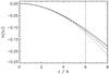 |
Fig. 1 Spatial damping profile for the first 8 wavelengths for ρ0/ρe = 1.4 and ϵ = 0.1. The solid line represents the full analytical solution of Hood et al. (2013) while the dashed and dotted lines represent the approximations given by Eqs. (2) and (8), respectively. The vertical dashed line is the height given by Eq. (10). |
If we substitute Eqs. (3) and (5) into Eq. (7), we obtain  (9)which can be rearranged as
  (10)This shows that the height of the switch in profiles (in terms of the number of wavelengths) depends only upon the ratio of densities. This information can be used to inform an observer as to which analytical formula is most appropriate for the seismological inversion. For example, for density contrasts above ρ0/ρe = 3, the switch occurs before h = 2λ and so the Gaussian profile is not appropriate for use as seismological inversion. On the other hand, for low density contrasts ρ0/ρe < 2, the Gaussian profile applies to the first 3 or more wavelengths (which is the typical number of observed wavelengths) and so the exponential profile is not appropriate for inversions. This is demonstrated by Fig. 2 which shows 1/κ as a function of ρ0/ρe.
Note that for a different density profile (not the linear change from ρ0 to ρe considered here), there may be a remaining constant of proportionality in Eq. (7). Additionally, we expect h to depend upon the profile of the driver since in the case of driving with the exact normal mode we must obtain h → 0.
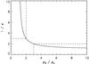 |
Fig. 2 Number of wavelengths after which the switch to the exponential damping profile occurs (1/κ) as a function of the density contrast ratio ρ0/ρe. For ρ0/ρe < 2 the Gaussian damping profile is expected to dominate the observed signal. For ρ0/ρe > 3 only the first 1–2 wavelengths exhibit the Gaussian damping behaviour. |
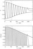 |
Fig. 3 General spatial damping profile for P = 24 s, ϵ = 0.2 and ρ0/ρe = 2. The solid lines show the numerical simulation of the damped kink mode and the analytical damping envelope given by Eq. (6). The dashed vertical line shows the change from Gaussian to exponential damping regimes, located at h = 3λ (see Fig. 2). |
An example of this general spatial damping profile is shown in Fig. 3. The top panel shows the transverse velocity vr at the centre of the loop r = 0 as a function of height or propagation distance z. The amplitude decreases with z as energy is transferred by mode coupling to azimuthal perturbations vθ in the inhomogeneous layer r ~ R. The envelope of the oscillation is the general spatial damping profile given by Eq. (6), with the location of the switch between approximations h = 3λ (Eq. (10)) denoted by the vertical dashed line. The lower panel shows the same velocity profile and envelope on a logarithmic scale. This makes the switch between Gaussian and exponential profiles easier to see, as the corresponding behaviour is either quadratic or linear, respectively. The dotted line shows what the Gaussian damping profile would look like if extended to heights z > h, and the dot-dashed line shows the extrapolation of the exponential profile back towards z → 0. It is clear that this hybrid or general spatial damping profile combines the best aspects of the Gaussian and exponential profiles to produce an envelope which is accurate for all z. Note that the leading edge of the wavetrain does not follow either profile, as described in detail by Hood et al. (2005).
Previous studies using damping of kink oscillations for seismology (e.g. Ruderman & Roberts 2002; Goossens et al. 2002) have focussed on the use of the exponential damping profile. The single fitted parameter Ld can have various combinations of inhomogeneous layer width and density contrast and so the inversion problem has infinite solutions, though bounding values can be estimated (e.g. Arregui et al. 2007; Goossens et al. 2008, 2012b). There is also a constant of proportionality that depends on density profile inside inhomogeneous layer. For the general spatial damping profile presented here, we have three fitted parameters; Lg, h and Ld. We can therefore in principle (for data of sufficient quality) obtain results for both the layer width and density contrast, plus the density profile.
3. Parametric study
In this section we will consider the dependence of the spatial damping profile upon the period of oscillation P, and the density structure parameters ϵ and ρ0/ρe.
Numerical simulations for various combinations of parameters were performed using a Lax-Wendroff code to solve the linear MHD equations in cylindrical coordinates. The lower boundary is driven harmonically with velocity perturbations that correspond to moving the loop footpoint back and forth about its equilibrium. This is a general driver that is continuous and does not assume the kink normal mode structure (see Pascoe et al. 2012 for detailed discussion).
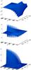 |
Fig. 4 Snapshots of vr (top), vθ (middle) and |
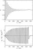 |
Fig. 5 vr at the centre of the tube (top) and vθ at the centre of the inhomogeneous layer (bottom) for the simulation in Fig. 4. The lower panel also shows |
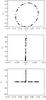 |
Fig. 6 Poynting vector hodograms for the dominant perturbations at low z (top) and high z (middle). The bottom panel shows the superposition of the two behaviours on the same scale. |
Figure 4 shows various snapshots for a simulation with P = 48 s, ϵ = 0.2 and ρ0/ρe = 5. The top and middle panels show vr and vθ, respectively, as functions of r and z. (Note that these plots do not show the full numerical domain.) For small z the signal in the tube interior is dominated by vr and vθ decaying, and a cut along the tube axis shows the decay of vr with z (see Fig. 5), the description of which is the focus of this paper. It can be seen that the dependence of vθ on r and z is very different to that of vr. Of particular interest is the growth of vθ with z in the inhomogeneous layer, which is shown in the bottom panel of Fig. 5. The growth in z of vθ and its saturation is matched by the decay of vr as energy is exchanged between various perturbations. The bottom panel of Fig. 4 shows  , where Ew is the wave energy density. At low z the energy is concentrated in the high density core of the tube, and at larger z it is focussed in the inhomogeneous layer. Cally & Hansen (2011) consider the case of mode conversion at a reflection level in a stratified atmosphere, in which only a fraction of the energy is exchanged.
The flow of energy in the evolving waves can be studied using the Poynting vector S, and in Fig. 6 we show hodograms of ( ,
, ) at two different locations. The top panel shows the hodogram plotted for the point r = 0.85 z = 22.7, i.e. at low z and in the core of the tube. Not surprisingly energy always flows along the tube (Sz > 0). Significantly Sr is nonzero, and so the wave is capable of transporting energy perpendicular to the background magnetic field. This is a feature characteristic of compressional magneto-acoustic waves. Note that Sr has a net positive value since these perturbations feed energy from the interior of the tube to the inhomogeneous layer.
The middle panel of Fig. 6 shows a Poynting vector hodogram for z = 478 where the compressional vr perturbations have decayed and the solution is dominated by the saturated vθ signature. Consequently, the hodogram is generated at the centre of the inhomogeneous layer (r = 1). The hodogram shows negligible Poynting vector perpendicular to the background magnetic field, whilst there is an intense field-aligned Poynting vector which is the familiar classic signature of an Alfvén wave. The scales of the axes in the top and middle panels are very different, and so to stress how the wave character has changed with z we superpose the two hodograms in the bottom panel of Fig. 6. At low z our simulation has compressional disturbances that transport energy along the tube but also, crucially, feed energy radially into the inhomogeneous layer. Once in the inhomogeneous layer the wave transports energy along the background field in a fashion reminiscent of Alfvén waves.
The wave dominated by vθ at large z has some other interesting characteristics. The bottom panel of Fig. 5 has  superposed on vθ as a dotted line. For nearly all z the two lines are indistinguishable (their difference is plotted as a dashed curve), which is yet another feature characteristic of propagating Alfvén waves.
It is also interesting to look at the radial structure of vθ at large z, which is shown in Fig. 7 for two values of z denoted by the dashed lines in Fig. 5. The numerical results in Fig. 7 clearly show that at larger z the waves have smaller spatial scales perpendicular to the background magnetic field. The phase structure of these waves was studied by Allan & Wright (2000) in a Cartesian geometry. They showed how the reduction in radial structure was described well by the process of Alfvén wave phase-mixing (e.g., Heyvaerts & Priest 1983).
Hence it appears our simulation fields have the character of magneto-acoustic modes at low z and are converted to perturbations at larger z that have properties similar to propagating Alfvén waves (see also Goossens et al. 2012a). This process itself does not dissipate energy, though dissipation may occur later, especially due to the large gradients produced by phase-mixing.
In the following simulations, the numerical domain covers r = [0,6R] and for z it scales according to the period so that 10 periods of oscillation can be accommodated z = [0,10CAeP] . Convergence tests with the radial boundary located up to 24R typically affected results by less than 5%. The typical resolution is 2400 × 3000 grid points, with convergence tests performed with 4800 × 6000 grid points. For the various simulations, R = 1, ρe = 1 and CAe = 1 were kept constant while P, l and ρ0 were varied. The simulation ends at t = 10P at which point the spatial damping profile can be investigated by considering vr as a function of z at the centre of the loop r = 0. Note that although we generate a damped signal composed of 10 wavelengths (e.g. Fig. 3), only up to 9 are considered for fitting. For the first period of oscillation (corresponding to the wavelength at highest z), the approximation of a harmonic signal is poor. Consequently, this period does not damp at the same rate as the later stage of the signal (Hood et al. 2005) and is therefore ignored.
3.1. Period of oscillation
Equation (3) can be rewritten to demonstrate the period dependence as 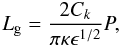 (11)where we have used λ = CkP (long wavelength limit).
The frequency-dependence of the exponential spatial damping profile was investigated by Terradas et al. (2010) and Verth et al. (2010). Eq. (5) can similarly be written as  (12)The fact that the damping length scale (for both damping regimes) is proportional to the period of oscillation means that mode coupling acts as a low pass filter, with higher frequency components being damped at lower heights. This was demonstrated by Terradas et al. (2010) for the exponential spatial damping profile and is also true for the Gaussian spatial damping profile. Note that these results are based on the applicability of the long wavelength or thin tube approximation. Section 5 considers the effect of dispersion when this approximation no longer applies.
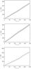 |
Fig. 8 Damping length scales Lg (triangles) and Ld (squares), and the height h (crosses) as a function of the period of oscillation P for numerical simulations with ϵ = 0.3 and ρ0/ρe = 2. The dotted lines show the analytical dependence given by Eqs. (11), (12) and (7), respectively. |
Figure 8 (top panel) shows the Gaussian damping length scale Lg as a function of the period of oscillation P. The dotted line shows the analytical dependence given by Eq. (11). The symbols are the results of numerical simulations with ϵ = 0.3 and ρ0/ρe = 2. Figure 8 also shows the exponential damping length scale Ld and the height h of the change from Gaussian to exponential damping profile, along with their analytical dependences given by Eqs. (12) and (7), respectively. The numerical length scales were calculated using a least squares fit of a general spatial damping profile as given by Eqs. (6) and (7) to the maxima and minima of the oscillation. The fitted values are in good agreement with the analytical dependences. Since each spatial damping profile is the same except for a linear scaling of the z axis with P, each period is fitted well with small errors. The error is largest for h since this is sensitive to errors in both damping length scales.
3.2. Inhomogeneous layer width
Equations (3) and (5) give the dependence of the damping length scales on the inhomogeneous layer width as  , Ld ∝ 1/ϵ and h independent of ϵ. Figure 9 shows Lg, Ld and h as a function of ϵ for numerical simulations with P = 24 s and ρ0/ρe = 2. We demonstrated in Sect. 3.1 that Lg,d ∝ P and so here we use a short period for numerical efficiency. Again the simulations are in good agreement with the analytical dependences.
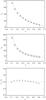 |
Fig. 9 Damping length scales Lg (triangles) and Ld (squares), and the height h (crosses) as a function of the inhomogeneous layer width ϵ for numerical simulations with P = 24 s and ρ0/ρe = 2. The dotted lines show the analytical dependence given by Eqs. (3), (5) and (7), respectively. |
3.3. Density contrast
Equations (3) and (5) give the dependence of the damping length scales on the density contrast as Lg,d ∝ 1/κ. Figure 10 shows Lg, Ld and h as a function of the density contrast ρ0/ρe for numerical simulations with P = 120 s and ϵ = 0.15. The damping length scales have an asymptotic dependence that is well reproduced by the numerical fits. Note that for these simulations we have chosen to use a longer period than in Sect. 3.2 in order to avoid the effects of kink mode dispersion, which becomes important when the wavelength is short and is discussed in detail in Sect. 5.
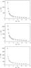 |
Fig. 10 Damping length scales Lg (triangles) and Ld (squares), and the height h (crosses) as a function of the density contrast ρ0/ρe for numerical simulations with P = 120 s and ϵ = 0.15. The dotted lines show the analytical dependence given by Eqs. (3), (5) and (7), respectively. |
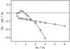 |
Fig. 11 Error in seismologically inferred density from fitting Gaussian (triangles) and exponential (squares) spatial damping profiles. P = 120 s and ϵ = 0.3. |
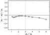 |
Fig. 12 Error in seismologically inferred density from fitting an exponential damping profile to all but the first 2 wavelengths. P = 120 s and ϵ = 0.3. |
4. Seismological inversions
In this section we will demonstrate the use of the proposed spatial damping profile (Sect. 2) as a seismological tool. First we will consider the use of observations of damped kink modes in order to determine the density contrast ratio present, and then as a method of determining the transverse length scale of the density profile (i.e. as a tool to reveal possible sub-resolution structuring).
In the case of fitting to the numerical simulations in Sect. 3, the numerical simulations provide sufficient data to be able to recognise both the Gaussian and exponential damping regimes and apply the general spatial damping profile (Eq. (3)) accordingly. Observational data is often not of sufficient quality to apply this method, and so in this section we will consider simpler fitting methods based on only a Gaussian (Eq. (2)) or exponential (Eq. (4)) fit and consider when each approximation is appropriate.
4.1. Determining the density contrast
In this section we consider the loop density calculated by means of seismological inversion (ρS) from our numerical data. Figure 11 shows the error in the seismological inversion (ρS − ρ0)/ρ0 when fitting the signal (9 wavelengths) to a Gaussian (triangles) or exponential (square) spatial damping profile, as given by Eqs. (2) and (4), respectively. In the limit of ρ0/ρe → 1, we have very weak damping, with Lg,d → ∞. In this limit, the damping envelope can be described by either damping profile and both fits tend to the correct value. For density contrasts that are sufficiently large to provide significant damping, the spatial damping profile will be some combination of both Gaussian and exponential damping profiles as described in Sect. 2. Consequently, attempting to fit a single damping profile to the whole signal will produce significant errors due to the effect of points not following that particular profile influencing the fit.
The error in the density calculated from the Gaussian fit increases significantly once the density contrast increases past ρ0/ρe ≈ 2.5 and the exponential damping regime starts to become dominant.
For illustrative purposes, Fig. 12 shows an improved exponential fitting method based on taking the presence of the Gaussian damping regime at lower heights into account. This example ignores the first two wavelengths of the oscillation at low z which will be at least partly affected by the Gaussian damping regime for all density contrasts. The vertical dotted line denotes the density contrast at which the change from the Gaussian damping profile to the exponential damping profile occurs after 2 wavelengths (see Fig. 2). In this region of ρ0/ρe ~ 3, this method produces very accurate estimates of the density contrast. The error increases for low densities for which the Gaussian damping regime extends significantly past the first 2 wavelengths. The error also increases for much larger density contrasts as the damping becomes very strong. Here, the approximation of weak damping, upon which the analytical expressions are based, no longer applies.
Despite this method producing good estimates over a range of density contrasts, it is only intended to illustrate the importance of applying the spatial damping profile suitable for the height observed. The practical application of such a method is likely to be limited by observational constraints. Observed oscillations often have a very low signal quality. The number of wavelengths that can be observed for a propagating wave may be limited by the length of the structure in which it propagates. The angle of the structure might also limit the observable portion. Both propagating and standing waves often have a low number of observable wavelengths/periods due to strong damping which quickly damps the oscillation below detectable levels (e.g. Aschwanden et al. 2002; Schrijver et al. 2002). It is therefore not appropriate to discard data in this way, especially the initial wavelengths which are expected to have the largest amplitude and hence lowest error.
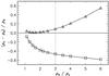 |
Fig. 13 Error in seismologically inferred density from fitting Gaussian (triangles) and exponential (squares) damping profiles to the first 2 wavelengths. P = 120 s and ϵ = 0.3. |
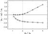 |
Fig. 14 Error in seismologically inferred density from fitting Gaussian (triangles) and exponential (squares) damping profiles to the first 3 wavelengths. P = 120 s and ϵ = 0.3. |
Figures 13 and 14 consider such a scenario of observations with a low signal quality. Figure 13 shows the Gaussian and exponential fits based on just the first 2 wavelengths. The vertical dotted line denotes the density contrast at which h = 2λ. Since these two wavelengths will both be in the Gaussian damping regime for ρ0/ρe ≤ 3, the Gaussian fit (triangles) produces a very low error in this range. For larger densities, part of the second wavelength will be influenced by the exponential damping regime and so the estimate becomes increasingly inaccurate. As expected, the exponential fit (squares) gives a poor estimate, except in the limit of very weak damping (ρ0/ρe → 1).
Figure 14 shows the same method as Fig. 13, except considering the first 3 wavelengths. The additional data points lead to a more accurate estimate from the Gaussian fit in the applicable range of density contrasts (less than that given by the vertical dotted line). However, this range is accordingly reduced to ρ0/ρe ≤ 2, and above this value the error increases more rapidly than in Fig. 13. The error for the exponential fit is reduced but still significant.
From these figures we can see that in the case of strongly damped oscillations with low signal quality, the Gaussian spatial damping profile is more appropriate for use as a tool for seismological inversion. However, it is also important to check that the inferred density contrast is consistent with the assumption that the Gaussian damping regime dominates the observed signal for the result to be reliable. Since the Gaussian fit overestimates the density contrast outside of its range of applicability (Figs. 13 and 14) this assumption can be qualified. For example, in Fig. 13, for ρ0/ρe = 4 the Gaussian fit for 2 wavelengths overestimates the density contrast by ≈ 20%, i.e. ρS = 4.8. This density would imply the Gaussian damping regime extends to 1/κ ≈ 1.5 wavelengths and so the Gaussian fit to 2 wavelengths will only be an approximation.
For comparison, for ρ0/ρe = 2 the Gaussian fit for 2 wavelengths overestimates the density contrast by ≈ 2%, i.e. ρS = 2.04. This density would imply the Gaussian damping regime extends to 1/κ ≈ 2.9 wavelengths and so the Gaussian fit to 2 wavelengths should be reasonable, as is the case.
Figures 13 and 14 also show how estimates based on an exponential fit tend to underestimate the density contrast, since the initial stage of the damping starts from a gradient of zero, rather than the maximum gradient assumed by the exponential spatial damping profile (e.g. Fig. 3).
4.2. Determining the inhomogeneous layer width
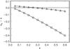 |
Fig. 15 Error in seismologically inferred inhomogeneous layer width from fitting Gaussian (triangles) and exponential (squares) spatial damping profiles to the first 3 wavelengths. P = 24 s and ρ0/ρe = 2. |
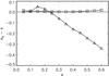 |
Fig. 16 Error in seismologically inferred inhomogeneous layer width from fitting Gaussian (triangles) and exponential (squares) damping profiles to wavelengths 4–6. P = 24 s and ρ0/ρe = 2. |
Using the damping of kink modes due to mode coupling as a seismological tool to determine the transverse scale of the density structure assumes that an estimate of the density contrast ratio is already known. In this case, the use of either a Gaussian or exponential damping profile to fit the data can be informed by the relationship demonstrated by Fig. 2.
Figures 15 and 16 show the errors in seismological estimates of ϵ for several methods in the case of a density contrast ρ0/ρe = 2. For this density contrast, we can expect the change from Gaussian to exponential damping regimes to occur at h = 3λ. Figure 15 shows the error in seismologically inferred density from fitting Gaussian (triangles) and exponential (squares) spatial damping profiles to the first 3 wavelengths of the oscillation. As expected, the Gaussian fit gives good estimates (mean error ≈ 10%) whereas the exponential fit gives a poor estimate (mean error ≈ 57%), since we expect the Gaussian damping profile to be dominant for these wavelengths.
If, instead, we consider the subsequent 3 wavelengths (4–6) as shown in Fig. 16, we see the situation reverses. Now (in this case) the exponential fit gives the better fit (mean error ≈ 4%), while the estimate based on the Gaussian fit is poor (mean error ≈ 29%). However, this method is again potentially limited in terms of practical application by observations having a small number of wavelengths observed, with the first ones being the most reliable, as discussed in Sect. 4.1.
4.3. Full seismological inversion
For data of sufficient quality, fitting the general spatial damping profile (Eq. (6)) allows the parameters h, Lg and Ld to be derived from which the density contrast and inhomogeneous layer width can both be calculated. The density contrast can be calculated from h using Eq. (10) and then Eqs. (3) and/or (5) can be used to find ϵ. By substituting Eq. (7) into Eq. (6) for z = h we can see that the amplitude of the signal at h can also be used to determine ϵ![Mathematical equation: \begin{eqnarray} &&A_h = \frac{A_0}{2} \left[ 1 + \exp \left( - \frac{\epsilon \pi^2}{4} \right) \right], \\[2mm] &&\epsilon = - \frac{4}{\pi^2} \ln{\left( 2 \frac{A_h}{A_0} - 1 \right)}. \end{eqnarray}](/articles/aa/full_html/2013/03/aa20620-12/aa20620-12-eq107.png)
5. Kink mode dispersion
The analytical spatial damping profiles given by Eqs. (2) and (4) are derived using certain mathematical approximations which are only valid in limited parameter ranges. In order for observed damped oscillations to be used as a reliable seismological tool, the same approximations should hold for the physical system being considered. In this section we present examples of kink oscillations that are not accurately described by our general spatial damping profile.
An assumption of the analytical theories is that the kink modes are in the long wavelength limit kR ≪ 1 and so the waves propagate at the kink speed Ck. Consequently the wavelength of the oscillation is λ = CkP. If the wavelength becomes sufficiently small that the long wavelength limit no longer applies, the wave speed is determined by the kink mode dispersion relation and the wave has a phase speed Vp < Ck. Accordingly, the wavelength is λ = VpP < CkP.
Such behaviour can be seen if we consider the dependence of the damping length scales with density contrast for short period oscillations. Figure 17 shows Lg, Ld and h as a function of the density contrast ratio ρ0/ρe for P = 24 s and ϵ = 0.2.
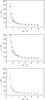 |
Fig. 17 Damping length scales Lg (triangles) and Ld (squares), and the height h (crosses) as a function of the density contrast ρ0/ρe for numerical simulations with P = 24 s and ϵ = 0.2. The dotted lines show the analytical dependence given by Eqs. (3), (5) and (7), respectively. |
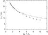 |
Fig. 18 Kink oscillation wavelength λ as a function of the density contrast ρ0/ρe. The dashed line shows the long wavelength limit λ = CkP. The crosses are the results of numerical simulations with P = 24 s and ϵ = 0.2. |
For low density contrasts, the wavelength is sufficiently long that the long wavelength limit applies and λ = CkP. As the density contrast increases, the wavelength decreases due to the lower internal Alfvén speed. For the larger density contrasts (ρ0/ρe ≳ 5) the data points have diverged significantly from the analytical curves. This effect is demonstrated by Fig. 18 which shows the dependence of the oscillation wavelength upon the density contrast. The dashed line represents the long wavelength approximation λ = CkP. We see that for the larger density contrasts (ρ0/ρe ≳ 5) the wavelength is significantly shorter than predicted by the long wavelength approximation. Since the analytical relation assumes a longer wavelength than the actual value, and Lg,d ∝ λ, the damping length scales are overestimated for these higher densities.
6. Discussion
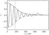 |
Fig. 19 Spatial damping profiles for P = 120 s, ϵ = 0.5 and ρ0/ρe = 2. The solid lines show the numerical simulation of the damped kink mode and the analytical damping envelope given by Eq. (6). The dashed vertical line shows the change from Gaussian to exponential damping regimes at h = 3λ. The thick dashed curve is an empirical Gaussian profile (Eq. (1)). |
It is instructive to reconsider the Gaussian profile proposed by Pascoe et al. (2012) in light of the results presented in this paper. This previous work suggested that the height up to which the Gaussian damping behaviour applied depended upon the inhomogeneous layer width ϵ. This can be reconciled by considering the conditions in order to reproduce the strong damping of kink modes as reported by Tomczyk & McIntosh (2012). The damping is greater for larger density contrasts and wider inhomogeneous layers. Pascoe et al. (2012) considered the case of strong damping achieved by means of a wide inhomogeneous layer and a low density contrast, e.g., their Fig. 1 is for ϵ = 2/3 and ρ0/ρe = 2. From the results of the present paper, we can understand that it is the low density contrast rather than the large inhomogeneous layer that is responsible for the dominance of the Gaussian regime over the exponential one. Figure 6 of Pascoe et al. (2012) shows two simulations with the same density contrast. In one case the inhomogeneous layer is thin and so the damping is weak, whilst in the other the damping is strong due to a wide layer and so the Gaussian behaviour dominates. In both cases the Gaussian behaviour applies for the same number of wavelengths, consistent with our Eq. (10).
Another point to consider is that the Gaussian fit considered by Pascoe et al. (2012) is an empirical one (Eq. (1)), whilst in this paper we consider a Gaussian profile (Eq. (2)) based on the analytical results of Hood et al. (2013). When the damping is strong and the density contrast is low, a Gaussian profile may be fitted to data up to and beyond h, however, for such an empirical fit it is not known how to relate the damping length scale Λg to the plasma parameters. An example of this is shown in Fig. 19 which shows a numerical simulation similar to that presented in Fig. 1 of Pascoe et al. (2012). The solid envelope shows the analytical damping profile given by Eq. (6). The thick dashed envelope is an empirical Gaussian profile (Eq. (1)), with  . Whilst the analytical expression (solid line) provides a slightly worse fit, it has the benefit of being applicable to a wide range of parametric values (Sect. 3) with known analytical relationships (Eqs. (3) and (5)) and can therefore be used as a seismological tool (Sect. 4).
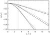 |
Fig. 20 Comparison of the general spatial damping profile (Eq. (6)) (solid lines) with the full analytical solution of Hood et al. (2013) (dashed lines). The upper pair of curves is for ϵ = 0.05. The middle and lower curves are for ϵ = 0.1 and ϵ = 0.2, respectively. For all curves ρ0/ρe = 2 i.e. h = 3λ (dotted line). |
Figure 20 compares the general spatial damping profile (solid lines) given by Eq. (6) with the full analytical solution of Hood et al. (2013) (dashed lines). The upper pair of curves is for ϵ = 0.05. The middle and lower curves are for ϵ = 0.1 and ϵ = 0.2, respectively. The density contrast is constant ρ0/ρe = 2 i.e. h = 3λ (dotted line) as given by Eq. (10). The location of the switch from Gaussian to exponential damping is therefore the same for each value of ϵ. However, the amount of damping that occurs over the distance h, and hence which damping profile is the dominant, does indeed depend upon ϵ.
6.1. Standing modes
The mode coupling process considered for propagating modes in this paper is a robust physical mechanism and the same behaviour is expected to apply for standing modes (with the appropriate changes in variables). Standing kink modes were observed (Aschwanden et al. 1999) long before the ubiquitous propagating kink waves, and have been analysed using normal mode analysis that predicts an exponential damping profile. However, such observations (e.g, Nakariakov et al. 1999; Ruderman & Roberts 2002; Goossens et al. 2002) usually assume that the individual loop structures seen to oscillate have a high density contrast, typically ρ0/ρe = 10, since the bright loops stand out against the background EUV emission. Such an assumption is consistent with the use of an exponential damping profile. For such a large density contrast, we expect the Gaussian behaviour to only apply for ~1.2 oscillations (Eq. (10)), which is insufficient for accurate analysis and might in any case be lost in the highly dispersive initial stage of oscillation that follows the excitation of global modes by impulsive events such as flares. Similarly, for prominence oscillations the density contrast is typically very high ~100–1000 and so we approach the asymptotic limit of the Gaussian damping profile applying for just a single period/wavelength (Fig. 2).
On the other hand, a density contrast of ≈ 1.2 was reported by Van Doorsselaere et al. (2008) for standing kink mode oscillations observed using Hinode/EIS. This particular oscillation was claimed to be undamped, which the authors proposed was an observational selection effect. Interestingly, Van Doorsselaere et al. (2008) used the FeXII 186/195 line ratio and CHIANTI to derive the density profile across the oscillating structure. This allows us to make some estimates of the damping rate we expect to observe in light of the results of the present paper.
The results discussed so far in this paper are for harmonically-driven propagating waves for which we consider the spatial damping profile. Following Pascoe et al. (2010) we can consider a corresponding damping timescale by considering a finite wavetrain propagating at a group speed Vg. Hence we obtain the change of variable t = z/Vg, where Vg = Vp = Ck in the long wavelength limit. For a standing mode decaying by resonant absorption with an exponential damping envelope we obtain from Eq. (12) 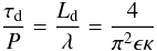 (15)as shown by, e.g., Ruderman & Roberts (2002). Similarly, we can consider a standing mode damping with a Gaussian envelope (see also Ruderman & Terradas 2012) and a characteristic damping time τg from Eq. (11) as
 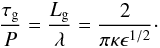 (16)The density profile presented by Van Doorsselaere et al. (2008) in their Fig. 3 has a peak electron density at the oscillating loop and is lower to each side of the loop. For the purposes of this approximation, we can consider the width of the inhomogeneous layer to be l = 2R i.e. ϵ = 2. This large value of ϵ is beyond the thin boundary approximation that the Gaussian and exponential damping profiles are based upon. However, the purpose of the following simple estimates is to demonstrate that the Gaussian damping regime naturally accounts for the observed weak damping. Van Doorsselaere et al. (2004) calculate that the exponential damping profile based on the TTTB approximation overestimates the damping by 25% when ϵ = 2.
For the reported density contrast of ρ0/ρe = 1.2 we have κ ≈ 0.09. Figure 2 of Van Doorsselaere et al. (2008) shows an oscillation in velocity with approximately 3.5 periods of oscillation. For the low density contrast observed in this oscillation, we expect the Gaussian damping profile to apply to the first 1/κ = 11 periods. If this oscillation is indeed damped by resonant absorption, we would expect it to be entirely dominated by the Gaussian damping profile. Other reported parameters for this oscillation are a period P = 296 s and a phase speed of 2.6 Mm/s. (Note the phase speed does not appear in Eqs. (15) and (16) but is useful for mode identification and these equations have assumed a long wavelength kink mode with Vp = Ck.)
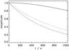 |
Fig. 21 Damping envelopes for the standing kink mode observed by Van Doorsselaere et al. (2008). The solid line shows the Gaussian damping profile (Eq. (16)) expected to dominate oscillations in such a low density (ρ0/ρe = 1.2) loop. The dashed line shows the exponential damping profile based on Eq. (15). The dotted line is an exponential damping profile with 25% weaker damping calculated by Van Doorsselaere et al. (2004) for a fully inhomogeneous model. |
Figure 21 shows damping envelopes for Gaussian and exponential profiles based on the observed parameters. The solid line shows the Gaussian damping profile based on Eqs. (2) and (16). The dashed line shows the exponential damping profile based on Eqs. (4) and (15). At t = 3.5P, the two analytical estimates show significantly different amounts of damping, with normalised amplitudes of approximately 0.8 and 0.2 for the Gaussian and exponential damping envelopes, respectively. This difference between Gaussian and exponential profiles is much larger that the 25% reported by Van Doorsselaere et al. (2004) for an exponential profile for a fully inhomogeneous model (indicated by the dotted line in Fig. 21).
By inspection of Fig. 2 of Van Doorsselaere et al. (2008), it is clear that the strong damping predicted by the exponential envelope is not present. However, the estimate based on the Gaussian damping envelope (Eqs. (2) and (16)) is much weaker. Determining the damping rate of the observed oscillation is complicated by the level of noise. The authors present a smoothed version of the data, which exhibits a trend to increasing (positive) velocities with time. As a rough estimate, we consider the trough-to-peak amplitude of the smoothed oscillation for the first half-period of oscillation and the last half-period. This produces estimates of approximately 2.0 and 1.6 km s-1, respectively, which is more consistent with the Gaussian damping envelope factor of 0.8 after 3.5 periods of oscillation than either of the exponential envelopes.
These approximations and estimates show that the damping rate of a low density contrast coronal loop is inconsistent with the rate predicted by the exponential damping profile (Eq. (4)). However, the results presented in this paper (Sect. 2) show that we expect this to be the case even if damping of kink modes by mode coupling is actually present. In the low density contrast regime, we expect the Gaussian damping profile (Eq. (2)) to be the dominant behaviour, and indeed the estimate based on such a profile is found to be consistent with the observational example.
7. Conclusions
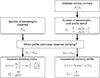 |
Fig. 22 Flowchart of a simple method to determine the appropriate spatial damping profile for seismology based on the number of observed wavelengths Nobs and an estimate of the density contrast ρ0/ρe. |
In this paper we have presented a general spatial damping profile for kink oscillations damped due to mode coupling. The profile (Eq. (6)) combines the exponential spatial damping profile, calculated as the asymptotic state of the system, at large heights (z > h) with a Gaussian profile, proposed numerically by Pascoe et al. (2012) and derived analytically by Hood et al. (2013), at low heights z ≤ h. The location of the switch between profiles, expressed as a number of wavelengths h/λ, is found to depend only upon the density contrast ρ0/ρe (and the driver profile).
The simple dependence of the height h upon the density contrast means that observers can consider whether the exponential or Gaussian damping profile is more appropriate for their data, as well as being a useful seismological tool. For observations with sufficient quality to apply the full general spatial damping profile, we can obtain a unique solution to the seismological inversion problem (Sects. 2 and 4.3), whereas fitting to a single exponential or Gaussian damping profile requires additional information about the density structuring. In cases of limited observational data where this is not possible, we considered several seismological methods (Sect. 4). Since current observational data is typically limited to oscillations with a low signal quality (i.e. only the first few wavelengths are reliably observed), we propose that the Gaussian damping profile is generally more appropriate for seismology, except when the density contrast is expected to be very high. This procedure is summarised in Fig. 22 which shows a flowchart of a simple method to determine which spatial damping profile is most appropriate for a particular observation. The method starts with an estimate of the density contrast. In the case that the damping length scale is being used to calculate the seismologically inferred density contrast, the result can be checked for consistency with the initial estimate as described in detail in Sect. 4.1. A different approach using a (linear) exponential damping profile for the seismological inversions was proposed by Goossens et al. (2012b). It is possible that combining the scheme proposed by these authors with our general damping profile would improve the seismological estimates.
In Sect. 5, we considered the case of kink mode dispersion in which the common assumption of the long wavelength limit no longer applies. The effect of the long wavelength approximation breaking down could be seen, and yet overall the behaviour was still quite well described by the analytical profiles. Considering various methods of using the profiles for seismological inversions in Sect. 4, we demonstrated simple yet robust methods for obtaining accurate (error ≲10%) estimates of some of the loop parameters. Indeed, even the less appropriate methods produced seismological estimates with errors less than a factor of 2. In this regard, the use of damped kink oscillations is a promising seismological tool, subject of course to sufficiently good data. This data would ideally resemble the numerical simulations presented here, i.e. accurate measurements of many wavelengths. However, we have shown that even just a few wavelengths can be sufficient for accurate inversions if they have sufficiently low noise.
In Sect. 6.1 we presented an example of a kink oscillation observed in a coronal loop with a low density contrast (Van Doorsselaere et al. 2008). This is the regime in which we expect the Gaussian damping profile to be most applicable and we found the estimate based on such a profile to be consistent with the observational example, whilst the exponential damping profile was inconsistent. The results presented in this paper may therefore account for the relatively high signal quality (i.e. weak damping) of that particular oscillation.
Acknowledgments
D.J.P. acknowledges financial support from STFC. I.D.M. acknowledges support of a Royal Society University Research Fellowship. The computational work for this paper was carried out on the joint STFC and SFC (SRIF) funded cluster at the University of St Andrews (Scotland, UK).
References
- Allan, W., & Wright, A. N. 2000, J. Geophys. Res., 105, 317 [NASA ADS] [CrossRef] [Google Scholar]
- Andries, J., van Doorsselaere, T., Roberts, B., et al. 2009, Space Sci. Rev., 149, 3 [NASA ADS] [CrossRef] [Google Scholar]
- Arregui, I., Andries, J., Van Doorsselaere, T., Goossens, M., & Poedts, S. 2007, A&A, 463, 333 [NASA ADS] [CrossRef] [EDP Sciences] [Google Scholar]
- Aschwanden, M. J., Fletcher, L., Schrijver, C. J., & Alexander, D. 1999, ApJ, 520, 880 [NASA ADS] [CrossRef] [Google Scholar]
- Aschwanden, M. J., de Pontieu, B., Schrijver, C. J., & Title, A. M. 2002, Sol. Phys., 206, 99 [NASA ADS] [CrossRef] [Google Scholar]
- Cally, P. S., & Hansen, S. C. 2011, ApJ, 738, 119 [NASA ADS] [CrossRef] [Google Scholar]
- Chen, L., & Hasegawa, A. 1974, Phys. Fluids, 17, 1399 [NASA ADS] [CrossRef] [Google Scholar]
- De Moortel, I., & Nakariakov, V. M. 2012, Roy. Soc. Lond. Phil. Trans. Ser. A, 370, 3193 [Google Scholar]
- De Moortel, I., & Pascoe, D. J. 2012, ApJ, 746, 31 [NASA ADS] [CrossRef] [Google Scholar]
- Goossens, M., Hollweg, J. V., & Sakurai, T. 1992, Sol. Phys., 138, 233 [NASA ADS] [CrossRef] [Google Scholar]
- Goossens, M., Andries, J., & Aschwanden, M. J. 2002, A&A, 394, L39 [NASA ADS] [CrossRef] [EDP Sciences] [Google Scholar]
- Goossens, M., Arregui, I., Ballester, J. L., & Wang, T. J. 2008, A&A, 484, 851 [NASA ADS] [CrossRef] [EDP Sciences] [Google Scholar]
- Goossens, M., Erdélyi, R., & Ruderman, M. S. 2011, Space Sci. Rev., 158, 289 [NASA ADS] [CrossRef] [Google Scholar]
- Goossens, M., Andries, J., Soler, R., et al. 2012a, ApJ, 753, 111 [NASA ADS] [CrossRef] [Google Scholar]
- Goossens, M., Soler, R., Arregui, I., & Terradas, J. 2012b, ApJ, 760, 98 [NASA ADS] [CrossRef] [Google Scholar]
- Grossmann, W., & Tataronis, J. 1973, Z. Phys., 261, 217 [Google Scholar]
- Heyvaerts, J., & Priest, E. R. 1983, A&A, 117, 220 [NASA ADS] [Google Scholar]
- Hollweg, J. V., & Yang, G. 1988, J. Geophys. Res., 93, 5423 [NASA ADS] [CrossRef] [Google Scholar]
- Hood, A. W., Brooks, S. J., & Wright, A. N. 2005, Proc. R. Soc. Lond. A, 461, 237 [NASA ADS] [CrossRef] [Google Scholar]
- Hood, A. W., Ruderman, M. S., Pascoe, D. J., et al. 2013, A&A, 551, A39 [NASA ADS] [CrossRef] [EDP Sciences] [Google Scholar]
- Ionson, J. A. 1978, ApJ, 226, 650 [NASA ADS] [CrossRef] [Google Scholar]
- Nakariakov, V. M., & Ofman, L. 2001, A&A, 372, L53 [NASA ADS] [CrossRef] [EDP Sciences] [Google Scholar]
- Nakariakov, V. M., & Verwichte, E. 2005, Liv. Rev. Sol. Phys., 2, 3 [Google Scholar]
- Nakariakov, V. M., Ofman, L., Deluca, E. E., Roberts, B., & Davila, J. M. 1999, Science, 285, 862 [NASA ADS] [CrossRef] [PubMed] [Google Scholar]
- Parnell, C. E., & De Moortel, I. 2012, Roy. Soc. Lond. Phil. Trans. Ser. A, 370, 3217 [Google Scholar]
- Pascoe, D. J., Wright, A. N., & De Moortel, I. 2010, ApJ, 711, 990 [NASA ADS] [CrossRef] [Google Scholar]
- Pascoe, D. J., Wright, A. N., & De Moortel, I. 2011, ApJ, 731, 73 [NASA ADS] [CrossRef] [Google Scholar]
- Pascoe, D. J., Hood, A. W., de Moortel, I., & Wright, A. N. 2012, A&A, 539, A37 [NASA ADS] [CrossRef] [EDP Sciences] [Google Scholar]
- Poedts, S., Goossens, M., & Kerner, W. 1989, Sol. Phys., 123, 83 [NASA ADS] [CrossRef] [Google Scholar]
- Poedts, S., Goossens, M., & Kerner, W. 1990, ApJ, 360, 279 [NASA ADS] [CrossRef] [Google Scholar]
- Ruderman, M. S., & Roberts, B. 2002, ApJ, 577, 475 [NASA ADS] [CrossRef] [Google Scholar]
- Ruderman, M. S., & Terradas, J. 2012, A&A, submitted [Google Scholar]
- Schrijver, C. J., Aschwanden, M. J., & Title, A. M. 2002, Sol. Phys., 206, 69 [NASA ADS] [CrossRef] [Google Scholar]
- Sedláček, Z. 1971, J. Plasma Phys., 5, 239 [NASA ADS] [CrossRef] [Google Scholar]
- Soler, R., Terradas, J., & Goossens, M. 2011a, ApJ, 734, 80 [NASA ADS] [CrossRef] [Google Scholar]
- Soler, R., Terradas, J., Verth, G., & Goossens, M. 2011b, ApJ, 736, 10 [NASA ADS] [CrossRef] [Google Scholar]
- Soler, R., Andries, J., & Goossens, M. 2012, A&A, 537, A84 [NASA ADS] [CrossRef] [EDP Sciences] [Google Scholar]
- Tataronis, J. A. 1975, J. Plasma Phys., 13, 87 [NASA ADS] [CrossRef] [Google Scholar]
- Terradas, J., Oliver, R., & Ballester, J. L. 2006, ApJ, 642, 533 [NASA ADS] [CrossRef] [Google Scholar]
- Terradas, J., Goossens, M., & Verth, G. 2010, A&A, 524, A23 [NASA ADS] [CrossRef] [EDP Sciences] [Google Scholar]
- Tomczyk, S., & McIntosh, S. W. 2009, ApJ, 697, 1384 [NASA ADS] [CrossRef] [Google Scholar]
- Tomczyk, S., McIntosh, S. W., Keil, S. L., et al. 2007, Science, 317, 1192 [NASA ADS] [CrossRef] [PubMed] [Google Scholar]
- Van Doorsselaere, T., Andries, J., Poedts, S., & Goossens, M. 2004, ApJ, 606, 1223 [NASA ADS] [CrossRef] [Google Scholar]
- Van Doorsselaere, T., Nakariakov, V. M., Young, P. R., & Verwichte, E. 2008, A&A, 487, L17 [NASA ADS] [CrossRef] [EDP Sciences] [Google Scholar]
- Verth, G., Terradas, J., & Goossens, M. 2010, ApJ, 718, L102 [NASA ADS] [CrossRef] [Google Scholar]
- White, R. S., & Verwichte, E. 2012, A&A, 537, A49 [NASA ADS] [CrossRef] [EDP Sciences] [Google Scholar]
All Figures
|
Fig. 1 Spatial damping profile for the first 8 wavelengths for ρ0/ρe = 1.4 and ϵ = 0.1. The solid line represents the full analytical solution of Hood et al. (2013) while the dashed and dotted lines represent the approximations given by Eqs. (2) and (8), respectively. The vertical dashed line is the height given by Eq. (10). |
| In the text | |
|
Fig. 2 Number of wavelengths after which the switch to the exponential damping profile occurs (1/κ) as a function of the density contrast ratio ρ0/ρe. For ρ0/ρe < 2 the Gaussian damping profile is expected to dominate the observed signal. For ρ0/ρe > 3 only the first 1–2 wavelengths exhibit the Gaussian damping behaviour. |
| In the text | |
|
Fig. 3 General spatial damping profile for P = 24 s, ϵ = 0.2 and ρ0/ρe = 2. The solid lines show the numerical simulation of the damped kink mode and the analytical damping envelope given by Eq. (6). The dashed vertical line shows the change from Gaussian to exponential damping regimes, located at h = 3λ (see Fig. 2). |
| In the text | |
|
Fig. 4 Snapshots of vr (top), vθ (middle) and |
| In the text | |
|
Fig. 5 vr at the centre of the tube (top) and vθ at the centre of the inhomogeneous layer (bottom) for the simulation in Fig. 4. The lower panel also shows |
| In the text | |
|
Fig. 6 Poynting vector hodograms for the dominant perturbations at low z (top) and high z (middle). The bottom panel shows the superposition of the two behaviours on the same scale. |
| In the text | |
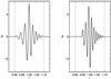 |
Fig. 7 vθ as a function of r at the values of z denoted by vertical dashed lines in Fig. 5. |
| In the text | |
|
Fig. 8 Damping length scales Lg (triangles) and Ld (squares), and the height h (crosses) as a function of the period of oscillation P for numerical simulations with ϵ = 0.3 and ρ0/ρe = 2. The dotted lines show the analytical dependence given by Eqs. (11), (12) and (7), respectively. |
| In the text | |
|
Fig. 9 Damping length scales Lg (triangles) and Ld (squares), and the height h (crosses) as a function of the inhomogeneous layer width ϵ for numerical simulations with P = 24 s and ρ0/ρe = 2. The dotted lines show the analytical dependence given by Eqs. (3), (5) and (7), respectively. |
| In the text | |
|
Fig. 10 Damping length scales Lg (triangles) and Ld (squares), and the height h (crosses) as a function of the density contrast ρ0/ρe for numerical simulations with P = 120 s and ϵ = 0.15. The dotted lines show the analytical dependence given by Eqs. (3), (5) and (7), respectively. |
| In the text | |
|
Fig. 11 Error in seismologically inferred density from fitting Gaussian (triangles) and exponential (squares) spatial damping profiles. P = 120 s and ϵ = 0.3. |
| In the text | |
|
Fig. 12 Error in seismologically inferred density from fitting an exponential damping profile to all but the first 2 wavelengths. P = 120 s and ϵ = 0.3. |
| In the text | |
|
Fig. 13 Error in seismologically inferred density from fitting Gaussian (triangles) and exponential (squares) damping profiles to the first 2 wavelengths. P = 120 s and ϵ = 0.3. |
| In the text | |
|
Fig. 14 Error in seismologically inferred density from fitting Gaussian (triangles) and exponential (squares) damping profiles to the first 3 wavelengths. P = 120 s and ϵ = 0.3. |
| In the text | |
|
Fig. 15 Error in seismologically inferred inhomogeneous layer width from fitting Gaussian (triangles) and exponential (squares) spatial damping profiles to the first 3 wavelengths. P = 24 s and ρ0/ρe = 2. |
| In the text | |
|
Fig. 16 Error in seismologically inferred inhomogeneous layer width from fitting Gaussian (triangles) and exponential (squares) damping profiles to wavelengths 4–6. P = 24 s and ρ0/ρe = 2. |
| In the text | |
|
Fig. 17 Damping length scales Lg (triangles) and Ld (squares), and the height h (crosses) as a function of the density contrast ρ0/ρe for numerical simulations with P = 24 s and ϵ = 0.2. The dotted lines show the analytical dependence given by Eqs. (3), (5) and (7), respectively. |
| In the text | |
|
Fig. 18 Kink oscillation wavelength λ as a function of the density contrast ρ0/ρe. The dashed line shows the long wavelength limit λ = CkP. The crosses are the results of numerical simulations with P = 24 s and ϵ = 0.2. |
| In the text | |
|
Fig. 19 Spatial damping profiles for P = 120 s, ϵ = 0.5 and ρ0/ρe = 2. The solid lines show the numerical simulation of the damped kink mode and the analytical damping envelope given by Eq. (6). The dashed vertical line shows the change from Gaussian to exponential damping regimes at h = 3λ. The thick dashed curve is an empirical Gaussian profile (Eq. (1)). |
| In the text | |
|
Fig. 20 Comparison of the general spatial damping profile (Eq. (6)) (solid lines) with the full analytical solution of Hood et al. (2013) (dashed lines). The upper pair of curves is for ϵ = 0.05. The middle and lower curves are for ϵ = 0.1 and ϵ = 0.2, respectively. For all curves ρ0/ρe = 2 i.e. h = 3λ (dotted line). |
| In the text | |
|
Fig. 21 Damping envelopes for the standing kink mode observed by Van Doorsselaere et al. (2008). The solid line shows the Gaussian damping profile (Eq. (16)) expected to dominate oscillations in such a low density (ρ0/ρe = 1.2) loop. The dashed line shows the exponential damping profile based on Eq. (15). The dotted line is an exponential damping profile with 25% weaker damping calculated by Van Doorsselaere et al. (2004) for a fully inhomogeneous model. |
| In the text | |
|
Fig. 22 Flowchart of a simple method to determine the appropriate spatial damping profile for seismology based on the number of observed wavelengths Nobs and an estimate of the density contrast ρ0/ρe. |
| In the text | |
Current usage metrics show cumulative count of Article Views (full-text article views including HTML views, PDF and ePub downloads, according to the available data) and Abstracts Views on Vision4Press platform.
Data correspond to usage on the plateform after 2015. The current usage metrics is available 48-96 hours after online publication and is updated daily on week days.
Initial download of the metrics may take a while.